Optimization problem definition
The linearly variable chord morphing and twist morphing concepts have been individually shown to be effective in improving the overall performance of the rotor2,4. But this improvement in performance came at the cost of a high elastic twist for both the concepts. The question arises, whether combining the two concepts results in synergizing their benefits, giving rise to better performance with minimum penalty or even reduction of the loads and vibrations. The combined morphing poser, by virtue of the large design space of possible morphing parameter values, lends itself to an optimization study. However, prior to combining the two morphing concepts, a detailed optimization study of the individual concepts for different missions is desired. The optimization algorithm chosen for the current work was the PSO due to its lesser function evaluations compared to other evolutionary algorithms. Details of the PSO implementation used in this work are given in 22, a brief summary of which is given in the sub-section below. The PSO algorithm is combined with S4, the in-house comprehensive analysis code at DLR26,27, which analyses helicopter rotors in hover and forward flight. S4 provides objective function values to the PSO algorithm.
Particle swarm optimization. In this method, a swarm of particles (population) is, initially, randomly distributed across the design space. The current position of each particle in the swarm (Equation 1) at any point in time is then updated using a velocity vector (Equation 2). Throughout the current work, a unit time step is used (Δt = 1).
The above equations are illustrated in Figure 6. Here, and are the position and velocity of particle p at iteration i; r1 and r2 are randomly generated factors ranging from 0 to 1, which differ for each particle and iteration; represents the best ever position of particle p where the objective function value is minimum, and corresponds to the global best position up to iteration i for the minimal value of the objective function for the whole swarm. w, c1 and c2 are optimization parameters limited to the 0–1 range. w is the inertia weight controlling the exploring abilities of the swarm. Large inertia weights allow for global exploration of the design space. c1 and c2 are trust parameters indicating, respectively, how much confidence the current particle has in itself and how much in the swarm.
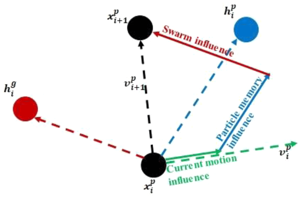
Figure 6. Position and velocity update for a swarm particle.
Objective function. Given the multidisciplinary nature of helicopter rotor analyses, the optimization study is proposed to be multi-objective. The following are the objectives selected for this optimization study: total rotor power required, P (performance criterion), blade tip elastic torsion, Φ (structural criterion) and N/rev hub vertical shear, Fz4/rev (vibration criterion). In mathematical terms,
The rotor power required has been chosen as an objective because the primary goal of the parent project SABRE is to improve the efficiency of the helicopter. The blade tip elastic twist is a critical parameter because it was found to be prohibitively high in the initial morphed designs, because of the change in torsional stiffness. Hence, this parameter was chosen as an objective. The tip elastic twist, being proportional to the root torsional moment, is also indicative of the magnitude of structural loads. The main rotor is the primary contributor of vibratory loads to the fuselage in the form of harmonics of the blade passage frequency. Since the Bo105 rotor, chosen for this work, is 4-bladed, the 4/rev harmonic of its vertical hub load, Fz, is a good measure of its vibratory loads. Thus, three critical aspects of helicopter rotor design, namely, performance, structural loads and vibratory loads, were considered for optimization in this work.
The multi-objective problem can be converted to a single-objective problem by building a composite objective function using the classical weighted sum method28 from the individual normalized, weighted objective functions:
where f is the composite objective function; fni is the normalizing factor; wi is the weighting factor.
The normalizing factors chosen for the three objective functions are: 350kW (for P), 2.5 deg (for Φ), and 500 N (for Fz4/rev).
Design constraints. Constraints are restrictions that must be satisfied to produce an acceptable design. The first requirement set here is that the rotor power required, P, at any velocity for the morphed rotor must be less than the corresponding rotor power (PBL) required for the baseline rotor at that velocity. Φ and Fz4/rev have upper constraints too. Thus,
Another requirement is that the rotor must be completely trimmed for any flight condition. This constraint is difficult to be translated into a mathematical form. It is implemented as a Boolean relation checking in an S4 output file for trim confirmation.
Design variables. The design variables used are the same as the morphing parameters. In the case of chord-morphing, the design variables and their corresponding limits are:
rh ∈ [0.4 - 0.7]; Δc ∈ [0% - 100%]; αd ∈ [0o - 15o]
The hinge location is limited to a maximum of 0.7 because longer lengths of the rear spar result in higher cross-sectional out-of-plane deformation of the morphed parts of the blade. Hinge locations less than 0.4 do not provide any substantial aerodynamic benefits because of the negligible morphed area. As will be seen in the next section, the dynamic response problem of the rotor is solved in the modal domain. For every change in the rotor structural properties, the modal information has to be recalculated. In order to keep the computational effort to reasonable levels, the design variable domains are discretized as follows:
rh ∈ [0.4 - 0.7] in steps of 0.02
Δc ∈ [0% - 100%] in steps of 12.5%
αd ∈ [0o - 15o] in steps of 5o
The following are the design variables for the case of twist morphing –
rt ∈ [0.22, 0.39, 0.56, 0.73, 0.9]; lt ∈ [0.0625, 0.125, 0.1875, 0.25, 0.5, 0.75]; Δθ ∈ [0.00, 0.22, 0.44, 0.66, 0.88, 1]
Thus, the first goal of the current optimization study is to find the combination of morphing parameters of a helicopter rotor which minimizes the performance, structural and vibration objective functions subject to some design constraints, for three different chosen mission profiles.
Analysis. It is to be noted that in the case of chord-morphing, the hinge location is a fixed parameter during a mission while the chord-extension and deflection can be changed as desired. These conditions make the morphed rotor optimization a two-level problem. The outer loop (Lo) decides the hinge location, rh, using a mission-level objective function. Within the outer loop, an inner loop (Li) determines the optimum combination of chord-extension, Δc, and chord-deflection, αd, for each velocity in a mission using the individual objective function. Thus, the outer and inner loops have their own objective functions and design variables:
Design variables:
XcLo = {rh}; XcLi = {Δc, αd}
Objective function:
Inner loop: f1(XcLi) = P; f2(XcLi) = Φ; f3(XcLi) = Fz4/rev
A composite objective function (fLi) is built using Equation 3.
This composite function is calculated for each velocity in a mission. Since the three objective functions are dissimilar quantities with different orders of magnitude, they are all non-dimensionalized with appropriate normalizing factors so that they can be summed together. The three objective functions are given equal weightage, wi = 0.333
Outer loop:
The outer loop objective function is calculated as the sum of composite objective functions of all velocities in a mission scaled by weighting factors, wvi, given in Table 2.
Similarly, the case of twist-morphing is also a two-level problem. However here, two parameters, namely, the radial location and the length of the torque-tube are fixed during a mission while the percent twist of the tube can be changed as desired. So rt and lt are determined in the outer loop while Δθ for each velocity is calculated in the inner-loop:
The inner and outer loop objectives for the twist-morphing case are determined in the same manner as for the chord-morphing case.
Following trade-off studies for convergence and duration, 10 particles were chosen as the population for the outer loop and 20 particles for the inner loop. The following values were taken for the optimization parameters (w, c1, c2): - (0.4, 0.1, 0.1) for the outer loop and (0.5, 0.2, 0.2) for the inner loop. These values satisfy the PSO parameter selection heuristic in 29.
The Bo105 main rotor blade with the airfoil NACA23012tab was selected as the baseline blade. The parameters for this baseline rotor blade are given in 2. The rotor had a rectangular blade geometry with a radius (R) of 4.92m, blade chord (C) of 0.27m and a linear twist of -8deg. The vehicle was powered by two engines with total power of 626kW. Important structural data distribution for the cross-section of this blade is shown in the Figure 7
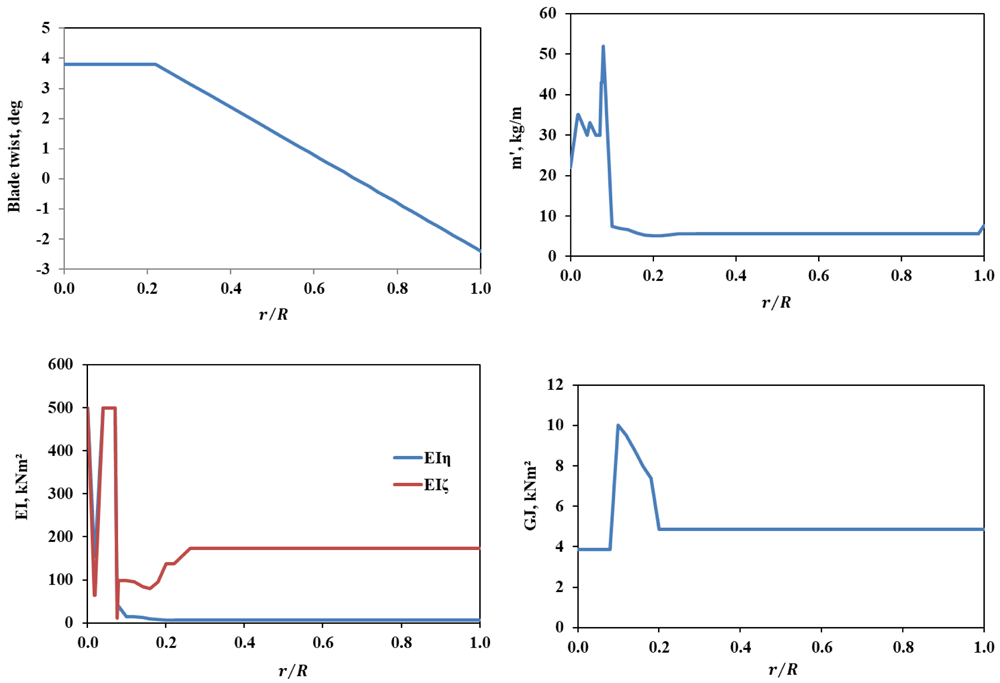
Figure 7. Cross-sectional properties of the baseline BO105 rotor blade.
Rotor comprehensive analysis. As already mentioned, the comprehensive analysis tool S4, a high resolution, nonlinear, unsteady aerodynamics code with elastic blade structural model, was used for the analysis of the isolated rotor for hover and forward flight conditions. For structural dynamics of the rotor, first, modal analysis was performed using the finite element method (FEM) based on the Houbolt–Brooks formulation30 which considers flap, lag and torsion degrees for the blade element. For the FEM, a radial resolution of 50 elements was chosen for the rotor blade and for the modal analysis, upto 10/rev natural frequencies were considered with 3-5 flap, 2-3 lag and 1-2 torsion modes. Next, for the dynamic response problem, the blade modes were subjected to generalized aerodynamic forces and generalized coupling forces from other modes like flap-torsion and flap-lag. The response problem was then solved using Runge–Kutta fourth order time-integration method until convergence was achieved. An azimuthal resolution of 1 deg was chosen for the analysis. S4 has an isolated rotor trim module, where the algorithm adjusted the collective pitch and cyclic pitch control inputs and the rotor shaft angle (for forward flight cases) until a trim goal was met.
Since the dynamic response problem was solved in the modal domain, for every change in the structural properties of the blade, a new modal analysis was required. Variation of the morphing parameters / design variables (Table 1) results in variation of structural properties of the blade and these were captured in the form of surrogate models which, essentially, take the form as in Table 3. It is to be noted that the beam formulation remains the same for the morphed blades too since morphing is modelled as only a change in the sectional properties.
Table 3. Properties table comprising the surrogate model.
station
mo. | r,m | r/R | Θ, deg | m', kg/m | ef, m | es, m | e0, m | if, m | Iη, m | Iζ, m | EIη, Nm2 | EIζ, Nm2 | EB1, Nm4 | EB2, Nm3 | GJ, Nm2 |
|---|
| | | | | | | | | | | | | | | |
| | | | | | | | | | | | | | | |
The structural properties of the rotor blade at multiple sections were calculated from 3D finite element models which consider the changes in shape of the section. The important changes in the structural properties of the surrogate models of the morphed configurations from those of the baseline blade are given in Refs. 2, 4. In order to reduce the costs of the optimization process, the modal information of all the rotor blades derived from different combinations of the morphing parameters were obtained in advance and used when needed by the code. The discretization of the domain space of the design variables for chord-morphing, as seen in the previous section, resulted in 16 x 9 x 4 = 576 surrogate models; while for twist-morphing, discretization resulted in 5 x 6 x 6 = 180 surrogate models.
Since chord-morphing resulted in a change of shape of the baseline NACA23012tab airfoil, each such case had to be treated as a new airfoil. As reported in 2, extensive CFD calculations were made for the two-dimensional aerodynamic coefficients of the modified airfoils in viscous mode over the range of Mach numbers and angles of attack expected to be experienced by the morphed sections of the rotor. Based on this fresh CFD data, unsteady aerodynamic formulation was synthesized for the aerodynamic coefficients as a function of the morphing parameters. The DLR unstructured Navier-Stokes solver TAU was used for all CFD computations31,32. The modified airfoil profile data was obtained from CAD models of the rotor blade and input to TAU. The test matrix for the computations was developed as below.
Test Matrix. Figure 8 shows the velocities experienced by different sections of the rotating rotor on the advancing and retreating sides in hover and in forward flight. The red triangle in the figure represents the chord-extension and spans from 0.22R – 0.6R. As can be seen in Figure 8b, the innermost parts of the rotor with chord-extension might experience reverse flow in the retreating side during forward flight.
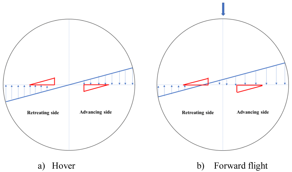
Figure 8. Sectional in-plane velocity distribution for the rotor blade.
As an illustration, for a 100% maximum chord-extension rotor at 70m/s, Table 4 shows the Mach numbers experienced by different spanwise sections on the advancing and retreating sides.
Table 4. Maximum and minimum Mach numbers.
| Cext | r/R | Mach no at max trim velocity |
|---|
| Advancing side | Retreating side |
|---|
| 100% | 0.22 | 0.36 | -0.07 |
| 75% | 0.32 | 0.42 | 0.00 |
| 50% | 0.41 | 0.48 | 0.06 |
| 25% | 0.51 | 0.55 | 0.12 |
| 0% | 0.60 | 0.61 | 0.18 |
Based on the illustration above, the following test matrix (Table 5) was setup for optimal CFD calculations. Five different chord-extension sections were considered. Each chord-extension case, apart from the 0%, included chord-deflections of 0 deg, 7.5 deg and 15 deg. It is to be noted that the 0% chord-extension rotor is aerodynamically the same as the baseline rotor. Also, negative Mach number indicates flow from trailing edge towards leading edge. The airfoil was given a slow sinusoidal pitching input for the analysis.
Table 5. Test Matrix.
| Chord-extension  |
Mach no  | | 0% | 25% | 50% | 75% | 100% |
| -0.2 | x | x | x | x | x |
| 0.2 | x | x | x | x | x |
| 0.4 | x | x | x | x | x |
| 0.5 | x | x | x | | |
| 0.6 | x | x | | | |
The unsteady aerodynamic formulation in S4 is based on the Leiss model33,34 where the aerodynamic equations are built from experimental data by superposition of three physical force sources resulting from fully separated flow as per Newton’s law, the separated circulatory flow, and the attached circulatory flow. Wagner and Kuessner functions were used to account for circulation lag effects in unsteady motion while dynamic stall is accounted for through a shift of the point of the static angle of attack assuming harmonic oscillation of the airfoil. This new formulation was then incorporated into S4. It is to be noted that such an exercise of deriving a new aerodynamic formulation is not required for twist-morphing because it does not result in a change of the airfoil shape.
S4 has been thoroughly validated as can be seen from literature. Data from wind tunnel experiments in the HART II test campaign, which utilized a hingeless Bo105 scaled model rotor, were used to corroborate the blade motion and sectional air loads of S426,27. The unsteady aerodynamic model for the baseline NACA23012tab airfoil in S4 was derived from data obtained from wind-tunnel tests. The new unsteady aerodynamic model in S4 which was synthesized from data obtained by CFD for the SABRE project was validated for performance and loads35 using data from test campaigns carried out at the NASA Ames Research Center 40-by-80-foot wind tunnel, utilizing the full-scale Bo 105 rotor36. The Mangler-Squire inflow model was used for the comprehensive analysis as noted in Ref. 2. The overall trends of the results from S4 have been found to be in good agreement with the test data.