1. Introduction
Mitigating anthropogenic climate change requires not only decarbonizing the energy sector, but also the reduction of greenhouse gases from the industry sector.1 Whereas the energy sector has great potential to meet the demand for heat and electricity from renewable sources, the decarbonization of the hard-to-abate industry, that is, heavy industries such as iron and steel, cement, and chemicals, is much more difficult and costly.2 The main challenge is the requirement of high process temperatures as well as greenhouse gas emissions from the inherent chemical process reactions.3 One viable solution for decarbonization is Geological Carbon Storage (GCS), as reported with high confidence in the Intergovernmental Panel on Climate Change (IPCC) report of 2023.4 For exploiting the full potential of GCS for these industries, the current global injection capacity of
needs to be upscaled by one order of magnitude towards a potential maximum capacity of
until 2030 and by another order of magnitude to
until 2050.1–5 Apart from these global storage objectives, the required storage capacity of a single GCS project is based on to the CO2 output of nearby high-emitting industrial plants. The common production rates of CO2 range from
for biofuel production6 to
from a medium-sized cement plant7 to the extreme case of
for one of the largest steel production plants in China.8 GCS is based on injection of CO2 from these industrial sources into a permeable reservoir rock at a depth below
which is confined by a low-permeability caprock.9,10 The injection of CO2 causes fluid pressure buildup, which may extend tens to hundreds of kilometers during a multi-decade injection. This migrating fluid pressure reduces the effective normal stress along preexisting fractures and/or faults, which lowers contact friction along preexisting fault planes.11 This phenomenon might result in seismic slip, depending on the prevalent shear stress in the system.12
This reactivation of preexisting faults is a major challenge to the large-scale implementation of GCS. Fortunately, induced seismicity is very unlikely to cause a leakage of CO2 by damaging the caprock due to the favorable geomechanical characteristics of the soft sedimentary GCS reservoirs.13,14 However, perceivable moment magnitudes
might occur due to fault reactivation within the crystalline basement below a reservoir. In an unfavorable geological setting as the one of the Castor underground gas storage site (Spain), these conditions led to three magnitude 4 seismic events. The project was terminated following this incident, resulting in a total cost to the Spanish taxpayer exceeding 4 billion euros.15,16 This example illustrates that successful management of induced seismicity is a prerequisite for large-scale implementation of GCS.
Operators can implement various strategies to mitigate the occurrence of perceivable seismic events with a maximum moment magnitude
.17 The predominant risk management framework to address induced seismicity is the traffic light system (TLS), which is voluntarily implemented by operators.18–20 The TLS is a decision scheme that defines distinct operational response categories, namely green, yellow, and red, corresponding to threshold values of decision variables, such as seismic rate
,
, and ground motion. Measurements of these decision variables within the green TLS category imply that the operation continues as planned. Within the yellow category, mitigation measures should be assigned, for example, a reduction of the pumping rate
. The red category indicates a major intervention that could involve the termination of the operation.18 For each color of the TLS, the threshold values of
,
, and ground motion are commonly based on site-specific risk and hazard assessment maps.21,22
A current limitation of the TLS is that its categories are associated with the monitored seismicity rather than the forecasted one.19,23–25 The rigid coupling of the operational response to the measured values of
and
is based on general empirical values that are not necessarily transferable to the geological conditions at the injection site. If the threshold values of
or
used in the TLS are underestimated, the operation could fall into the red category although there is no large-magnitude event about to happen. Thus, the injection may be unnecessarily stopped, resulting in an economic loss. An example is the incomplete reservoir stimulation at the enhanced geothermal system (EGS) site at Otaniemi (Finland) due to fixed injection limits based on the total injected volume.23–26 Alternatively, overestimation of the threshold values of
or
could result in operators missing the opportunity to adjust the flow rate in time, and therefore being unable to prevent an unexpected high-magnitude event. TLS also fails to prevent large-magnitude earthquakes occurring after the stop of injection, a common phenomenon in EGS, like at the EGS in Basel (Switzerland) with
27 and Pohang (South Korea) with
.28–30 Although such negative examples have not yet occurred in the GCS industry, we strongly recommend treating them as warning signs. Instead of using fixed threshold values for
or
within TLS, we firmly advocate investing in the development of accurate near-real-time induced seismicity forecasts to ensure the economic and social success of GCS projects.
Despite its significant potential, near-real-time forecasting of induced seismicity still requires major developments. This is because existing forecasting models either lack sufficient complexity to generate reliable forecasts (e.g., primarily statistical models) or are too computationally demanding for near-real-time calibration and execution (e.g., physics-based models).31 Statistical models have been applied and developed in the seismological community mainly based on the Gutenberg-Richter-Law and other decay principles similar to natural seismicity.32–35 The advantage of such probabilistic approaches is that they require relatively low computational resources and provide an immediate output of a target variable, such as
or
. At the same time, they do not consider triggering mechanisms based on fluid injection itself. The coupling with simplified physical relationships can be provided through an analytical solution in hybrid physical-statistical models, as Shapiro et al. (2002)36 show with their model for axisymmetric pressure diffusion. The simplified pressure front can be linked to the systems seismic response, allowing an estimate of the possible
.37 This assumption of pore pressure as main driver of induced seismicity allowed Langenbruch et al. (2018)38 to estimate
for
applied to Oklahoma’s oil fields (USA). At the same time, such purely hydraulic models are not applicable in fracture-dominated reservoirs where hydro-mechanical stress coupling dominates the seismicity.12–15,39 This shortcoming can be addressed by using multi-physical numerical models as input for probabilistic models instead. Traditionally, such complex physics-based models are mainly used to identify triggering mechanisms15–40 of induced seismicity or modeling injection scenarios to prevent such unfavorable events.41,42 In particular, numerical codes provide a high-resolution spatiotemporal distribution of state variables such as pressure, displacement and temperature based on physical laws.43,44 As deterministic numerical models do not adequately address the uncertainty of occurring seismicity, the relationship between state variables and observed seismicity is typically established through probabilistic or empirical relationships.45,46 Such hybrid workflows have been developed47,48 and applied to well-documented injection sites, as demonstrated by Dempsey and Suckale (2017)49 in Groningen (Netherlands), and Hill et al. (2024)50 in the Raton Basin (USA). However, empirical and analytical equations that define the relationships between state variables and seismicity, such as rate-and-state friction, face limitations in their general applicability. This is due to uncertainties in the distribution of the required model parameters, and the potential influence of neglected physical effects, such as fault lubrication.51
A promising option to complement these shortcomings can be provided by machine learning (ML) algorithms. Advancements have been made with regard to correlating measured data with target variables such as
and
. For example, ML has been successfully tested at scales where large data are available, namely the lab scale52–54 and the long time-series history of natural earthquakes. For the latter ones, De Vries et al. (2018)55 applied a deep neural network to forecast aftershock sequences over time and space. Although their method outperforms a compared physics-based model applied for natural earthquakes, the applicability has not been demonstrated for human-induced earthquakes where the main shocks themselves would be of major interest. Similarly, Saad et al. (2023)56 proposed a framework based on a Random Forest (RF) model for the spatiotemporal forecast of
and
. rf has also been applied to induced seismicity by Qin et al. (2022)57 to a large dataset from Oklahoma (USA), who analyzed the relationship between various operational features and the seismic rate
over time and space. Their hindcast proofs its applicability by successfully associating hydraulic data such as
, well pressure
, and data from the seismic catalog for the same time window.
While such retrospective analysis offers valuable insight into the correlations of operations and observed seismicity, a primary challenge lies in the forecast of
and
. Near-real-time prospective forecasting for seismicity is still a young domain, with great potential for development and knowledge transfer into the domain of subsurface fluid injection. Until now, some pioneering works have been published, using different features of time-series data, while usually splitting the data into a fixed training period and a forecasting period. For example, Li et al. (2023)58 used an artificial neural network to forecast the maximum magnitudes
based on the previously measured data from
at the example of the Tony Creek Dual Microseismic Experiment (Canada). Yu et al. (2023)59 used a lagged linear regression to forecast
based on injection rates. Similarly, Mignan et al. (2024)60 linked
to the injected volume based on the approach of Shapiro et al. (2011)37 by applying a ‘least absolute shrinkage and selection operator’ model. Using a more suitable architecture for time-series forecasting, Picozzi and Iaccarino (2021)61 passed features from a seismic catalog in a recurrent neural network to predict the preparatory phase of an
event.
Much of the previous work provides a framework that can be extended to near-real-time forecasting. However, most studies do not explore the potential of assessing their models’ continuous performance from the beginning of the injection operation.58–60 Therefore, we propose in this study a near-real-time forecasting workflow based on a random forest model that continuously assimilates new measurements and re-trains the model as new data are obtained. We establish our model utilizing data from the demonstration GCS injection site of the Illinois Basin Decatur Project (IBDP) (Section 5.2). These data are preprocessed with a shifted moving window approach as data-partitioning technique (Section 5.1). In Section 2, we describe the results of our forecast for the target variables, namely seismic event count
and
. An improvement in forecasting accuracy, highlighted by changes in feature importance and a better
score, is observed after the initial IBDP seismic event cluster. Subsequently, the forecast performance diminishes after the second cluster, probably due to the growing importance of fluid pressure diffusion into the far field of the reservoir. Following these results, we evaluate in Section 3 the model performance when using solely hydraulic data compared to using both hydraulic and seismological data. We also provide guidance on the optimal window length as a key parameter within our modeling framework. Finally, we assess the current model’s limitations and propose future development paths towards spatial forecasting. In this way, our work contributes a significant component for adaptive near-real-time forecasting of induced seismicity in GCS.
2. Results
We present our modeling results for forecasting the number of seismic events
and the maximum magnitudes
. Each of these two target variables is forecasted with a separate model, since the importance of the respective characteristic features varies significantly among them. We preprocess the training data of both models by binning the ground truth to moving windows, where we use a window length
. In addition, we set the window shift to
for every timestep (see
Figure 7). This seems a pragmatic choice, since the assimilation and evaluation of operational and seismological data at a project site are likely to follow a daily cycle. The initial model is trained with all data that are obtained within the first
days. The continuous forecast starts after this initial traing, which means that the model incorporates new data and is re-trained after each timestep (see
Figure 8).
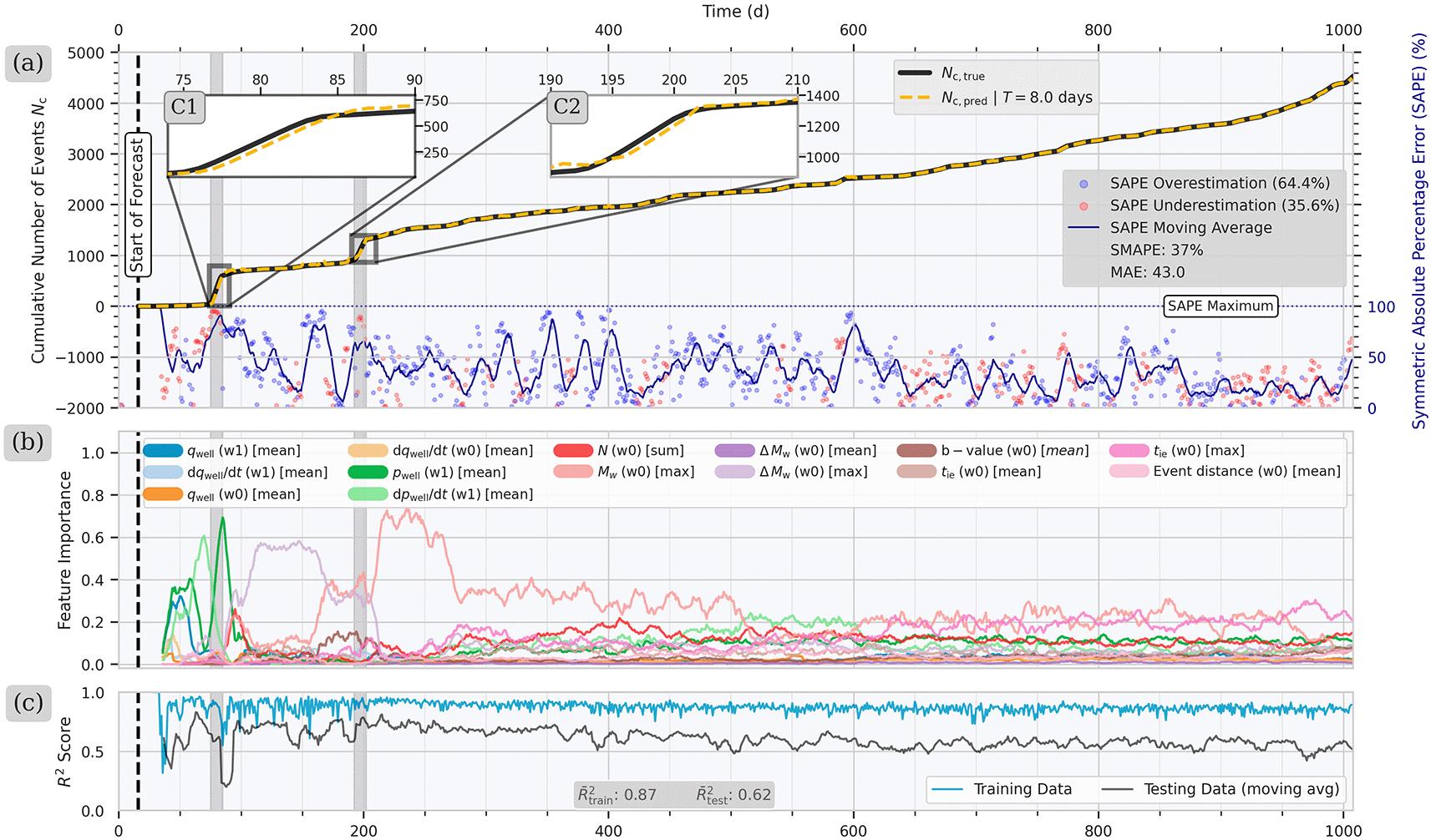
Figure 1. (a) Iterative forecast of the cumulative number of seismic events
for a window length of
days starting from day
with the ground truth
(black) and the forecast values
(dark yellow).
The Symmetric Absolute Percentage Error (SAPE) shows higher values after the first seismic cluster C1 in comparison to the period after of the second cluster C2. (b) The initially important training features are the hydraulic variables
and
, which are replaced after C1 by the seismic features
and
. (c) The
score for training (blue) and testing (black) decrease slightly in the period between C2 and the end of the injection.
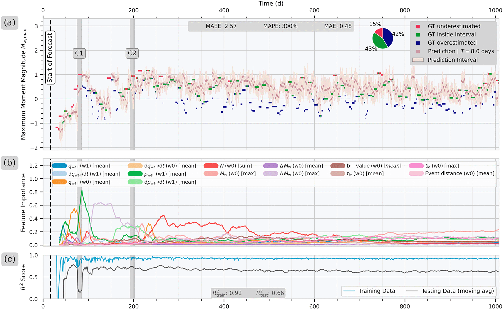
Figure 2. (a) Continuous forecast for the exponentially scaled maximum magnitude
for a window length of
days starting after 4 days of injection.
The forecasted values of
are in dark pink and the associated standard deviation in light pink. Values of
within the standard deviation are colored in green, while underestimates windows are colored in pink, and overestimated ones in blue. The pie chart in the upper-right corner summarizes the count of each category. (b) Feature importance values through time. The fluid pressure
is the most important feature after the onset of cluster C1, however it steadily decreases in importance as operation continues. (c)
score over time for the training data (blue) and testing data (black). The trend shows higher
scores after C1 and a slight decrease after day
.
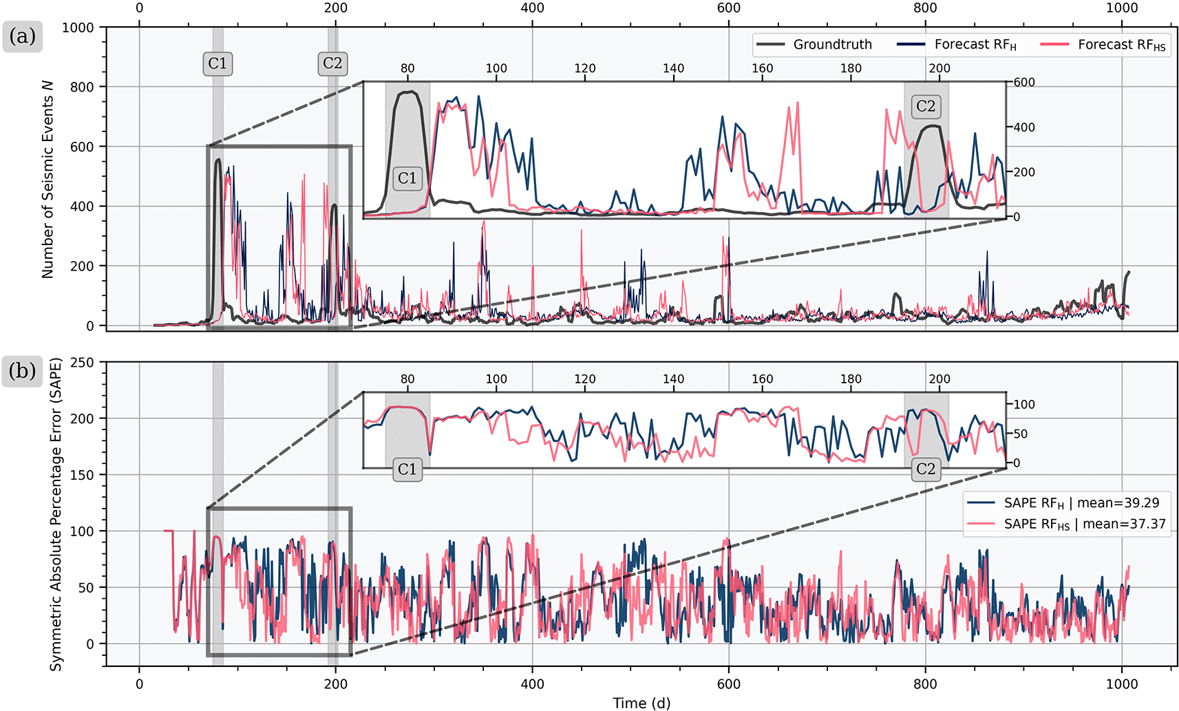
Figure 3. Comparison of forecasting performance for the number of seismic events
of model RFH with only operational input features versus model RFHS with operational and seismological input features.
(a) While both models forecast a similar number of seismic events (
) during the early times, RFHS shows less high-magnitude outliers over the total injection period. (b) For the Symmetric Absolute Percentage Error (SAPE), both models have the highest values during C1, while RFHS has again a better performance afterwards, especially in between C1 and C2.
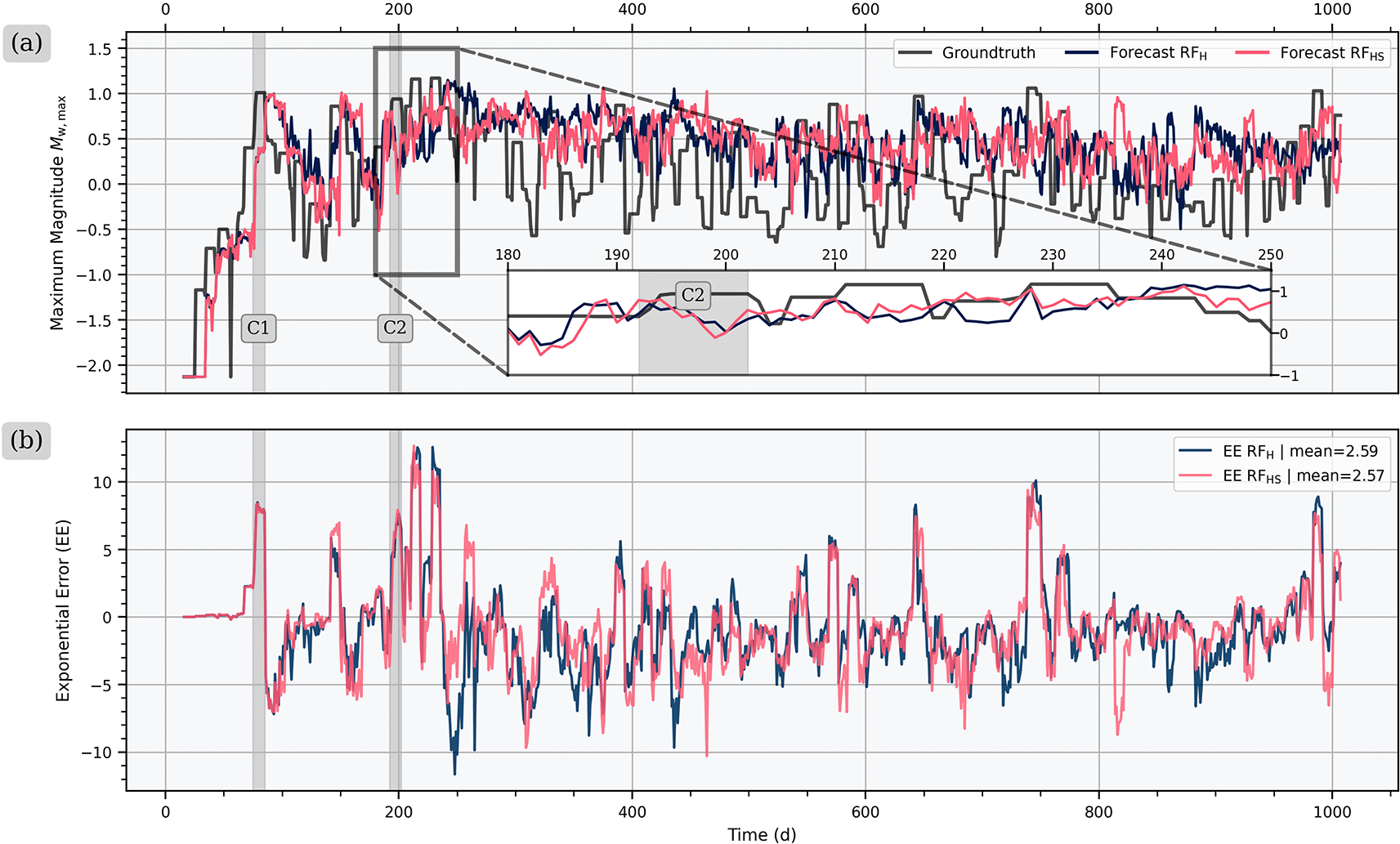
Figure 4. Comparison of forecasting performance for the maximum magnitude
of model RFH with only hydraulic input features versus model RFHS with hydraulic and seismological input features for (a)
and (b) the exponential error.
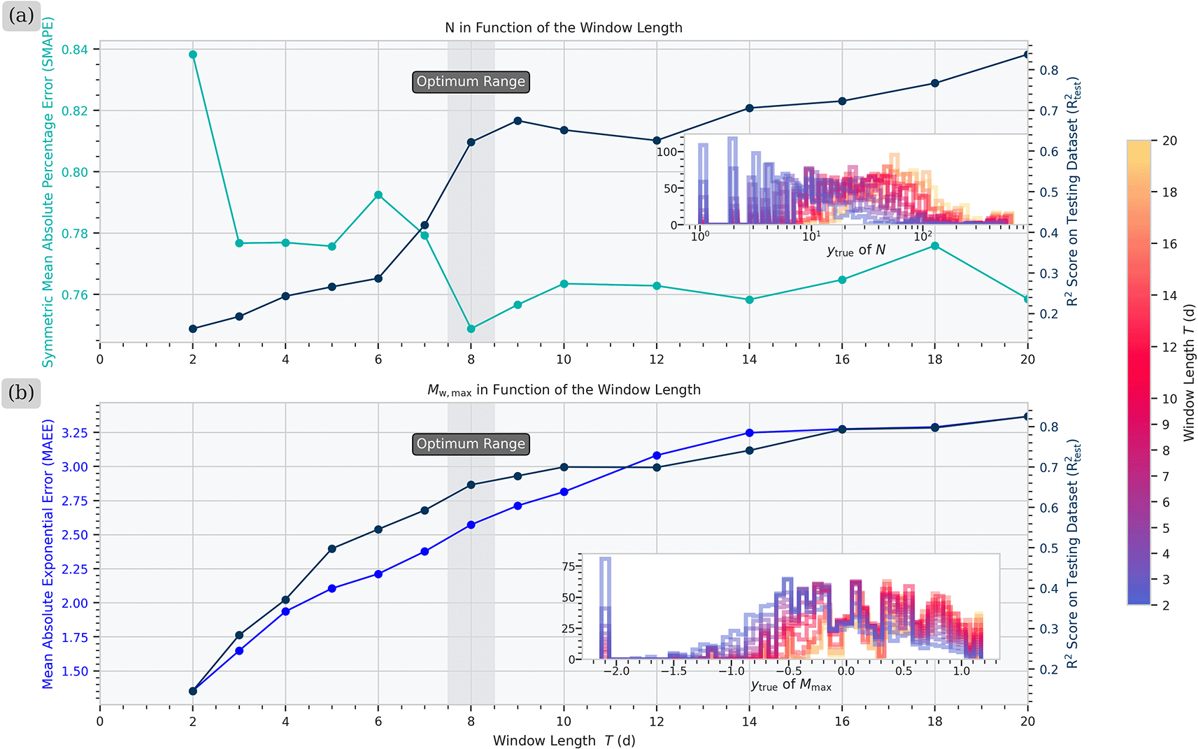
Figure 5. Evaluation of the influence of the window length
on the model performance for the forecast of (a)
and (b) and
.
(a) For the forecast of
, the trend of the Symmetric Mean Absolute Percentage Error (SMAPE), and
indicate an optimum of
days. (b) The increasing Mean Absolute Exponential Error (MAEE) and the plateau of
suggest
days as the optimal
for the forecast of
.
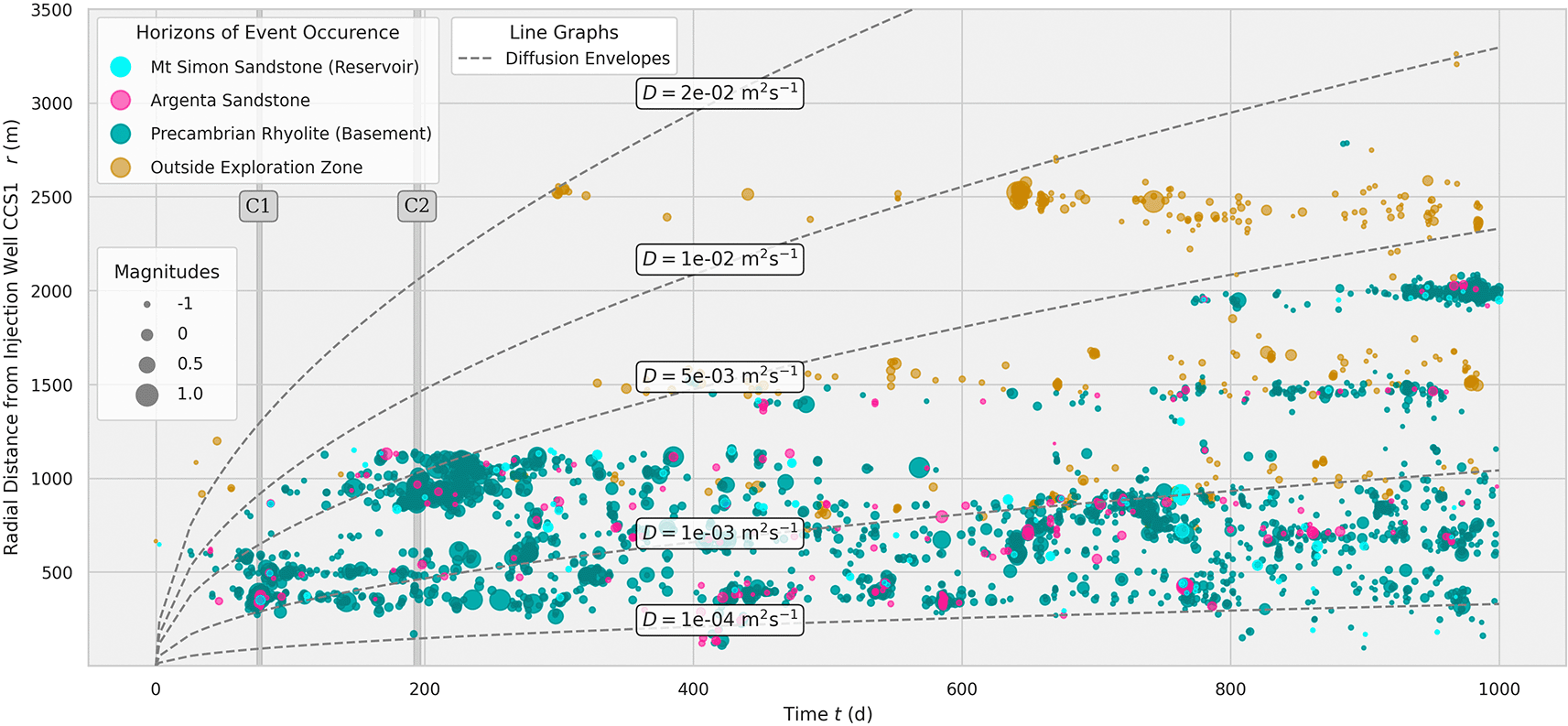
Figure 6. Spatiotemporal distribution of seismic events at the IBDP from the seismic catalog of Dando et al. (2021)67 in correlation to radially symmetric pore pressure diffusion envelopes.36
Most of the events happen in the Precambrian basement (teal). The radial diffusion envelopes (dashed lines) indicate that the seismicity locations can be correlated with a diffusion coefficient of
. The light-brown events could not be assigned to a horizon since they are located outside the boundaries of the reservoir model of Zaluski and Lee (2021).68
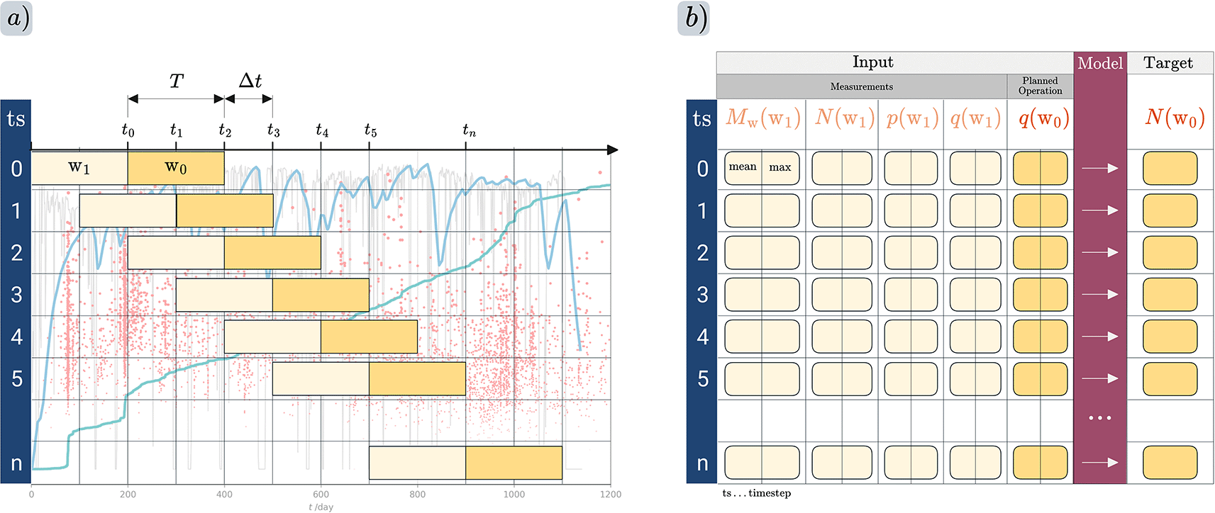
Figure 7. (a) Windowing approaches used to partition the training and testing data from the IBDP site.
For each timestep, measurements are assigned to window
while
for the future pseudo-planned operation and the seismological target variable, either
or
, are assigned to window
. Statistical metrics are calculated for each variable, including the mean and maximum of each window, as well as optionally the cumulative sum or difference over time, among other metrics. (b) Location of the model layer (dark red) that learns the relationship between the input features and the target features.
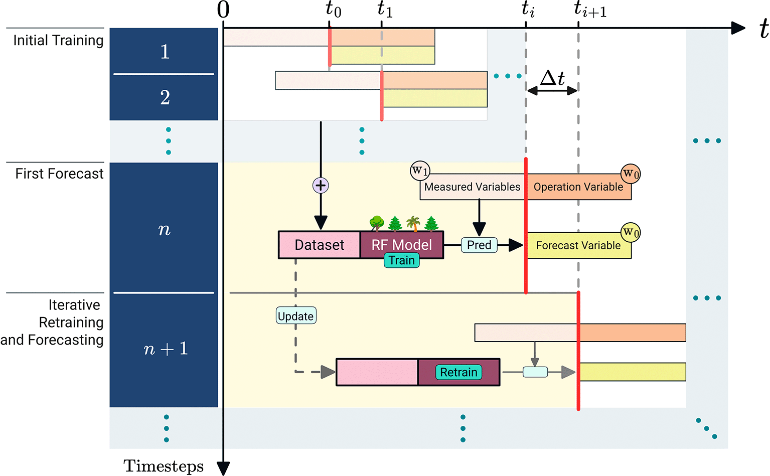
Figure 8. Real-time workflow for data assimilation and seismicity forecasting.
The workflow starts with an initial training with timestep
where the training dataset consists of
data points. The first forecast is made based on the measurements and the operation variable obtained until time
. The random forest model receives measured variables from window
, and an operation variable from window
as input features and learns their relationship to a forecast variable, for example, the cumulative number of seismic events
, for window
. Subsequently, the workflow continuously retrains the RF model with the latest obtained data for every new timestep.
2.1 Forecasting the seismic event count
We present the results of our continuous training and forecasting workflow for
in
Figure 1. In the cumulative graph of
, labeled as
, we compare the evolution of the binned ground truth as
(black line) and the model output as
(yellow dashed line). In addition, we use the Symmetric Absolute Percentage Error (SAPE) metric from Equation 2 to assess the forecasting performance, which is the most suitable metric for the given data range (see Extended Data S4 at Walter (2025)62). Regarding the evolution of our continuous forecast, we observe the first deviation from the ground truth during the first earthquake cluster C1 at
. As clearly visible in the zoomed inset figure of C1, the model output
underestimates
until C1 ends, which is also indicated by the dominantly red color of the SAPE. It reaches values up to
for C1 while the upper bound is
. After C1 ends,
overestimates
, shown by the mostly blue SAPE. For the subsequent cluster C2, the model also misses the onset of a sudden increase in the event rate. However, it adapts comparably faster to the transition from a high rate to a low rate of
at the end of the cluster, as shown in the zoomed plot for C2 in
Figure 1a and as the lower maximum error of
indicates. In general, the forecasting performance of our model improves after
days, which is indicated by the reduction in the moving average for 100 windows of SAPE (dark blue). In total, our model overestimates
in
of the windows while it underestimates
. Overestimation is generally more favorable by preventing negative effects on the project operation.
Apart from the apparent forecasting results, we provide insight into model training by displaying the evolution of feature importance and the
score over time in
Figure 1b and
Figure 1c, respectively. While using both hydraulic and seismological features for training, our forecasting workflow identifies the hydraulic features
and
as the two most important ones until the onset of C1. This observation implies that the seismicity in that stage is mostly related to pore pressure changes. However, the elevated SAPE values observed during this period indicate that this feature importance can only be partially relied upon. After C1, the maximum magnitude difference
is the dominant feature until day
. Then, the maximum magnitude
takes over shortly after the end of C2 with maximum values up to
. Both, the importance of
and subsequently
, could be correlated with static stress transfer caused during C1 and C2. The importance of
remains in the range of
during the period
, while the error range increases again with values up to
. Similarly, there is no clearly dominant input feature observable after day
, indicating that the model has difficulty relating the input variables to
. This observation is also supported by the evolution of the
score in
Figure 1c. The training score
reaches its highest values between C1 and C2 with
, while steadily decreasing afterwards. The
score behaves similarly, reaching
at C1 and shortly after C2, showing a similar decline just afterward. We assume that the initial increase of both values is related to the increasing amount of available data and to a more constant range of the distribution of
-values, while the following decrease might be due to pressure diffusion in the far field, which we discuss in more detail in Section 3.3.
2.2 Forecasting maximum magnitudes
For the forecast of the maximum moment magnitude
use principally the same input features, consisting of a combination of operational and seismological variables. A main challenge for modeling
is that underestimations of the future observed
could have more severe implications for the operation, in the worst case a cessation of the project, whereas an overestimation could only lead to a minor economic loss. We address this issue by scaling the target variable
exponentially via
, penalizing larger magnitudes more severely than smaller ones (see Equation 5). In this way, we achieve an underestimation rate of
and an overestimation of
(see pie chart in
Figure 2a). In comparison, an alternative realization of the model that uses
shows a fairly equal distribution of under- and overestimates with
and
, respectively (see
Figure 1 in Extended Data at Walter (2025)62).
When analyzing the temporal trends of
in
Figure 2a, the measured magnitudes exhibit a range of
with significant fluctuations within the injection period. The forecasted magnitudes show a similar range between
. From the start of injection until the end of the first cluster C1, our model underestimates most of the observed
values. Shortly after C1 occurred, it rather overestimates, although it produces a few accurate predictions around day
. During this time span, hydraulic features such as
and
have the highest importance with values of up to
. In between C1 and C2, the importance of the hydraulic features decreases while the maximum magnitude difference
becomes the most important. In the same time frame, the
score constantly increases to
, while showing a drop during C1. In comparison, the observed maximum magnitudes increase within
days after C2 up to
, when the forecast again shows a certain delay to adapt, as indicated by the red markers in
Figure 2a. The following period after day
shows a majority of correct forecasting or overestimation, when the event count
is the most conclusive input feature, while
again reaches values greater than
. Between day
and day
, the model fails to forecast an event with
, despite the overall satisfactory performance. During this period, no feature stands out as particularly important and the
score shows a slight decrease. Overall, the chosen forecasting model effectively reduces the underestimation of
by using exponential scaling, although the forecast accuracy still shows potential for improvement.
3. Discussion
3.1 Forecast comparison: Hydraulic-only versus hydraulic and seismological features
The performance of our near-real-time forecasting workflow is mainly influenced by the quality of the input features provided to the model. The forecast results for
(
Figure 1) and
(
Figure 2), presented in Section 2, were obtained by training the RF model on both hydraulic and seismological input features, following referred to as RFHS. To understand the impact of the seismic catalog on the model performance, we compare these results with a model called RFH, which only uses the hydraulic features
and
for training. This distinction may be of interest for operators of GCS projects since these hydraulic parameters can be more conveniently obtained in near-real-time compared to the preparation of a seismic catalog.
Table 1 lists the training features for each respective model, as well as several evaluation metrics for the forecast of
and
. For the forecast of
, the comparison of RFH and RFHS shows a slight, but not significant improvement of RFHS compared to RFH (see forecasting results of RFH for
in
Figure 2 and for
in
Figure 3 in Extended Data at Walter (2025)62).
Table 1. Comparing model evaluation metrics when using only hydraulic input features from the injection (RFH) versus also using the seismic catalog (RFHS).
GT is the ground truth.
|
|
|
|---|
| RFH | RFHS | RFH | RFHS |
|---|
| Input Features:
| | | | |
|
[mean] | x | x | x | x |
|
[mean] | x | x | x | x |
|
[mean] | x | x | x | x |
|
[mean] | x | x | x | x |
|
[mean] | x | x | x | x |
|
[mean] | x | x | x | x |
|
| | x | | x |
|
| | x | | x |
|
| | x | | x |
|
| | x | | x |
|
| | x | | x |
|
| | x | | x |
|
| | x | | x |
| Evaluation Metrics:
| | | | |
| Underestimate of GT | 40.9 | 35.6 | 14 | 15 |
| Overestimation of GT | 59.1 | 64.4 | 44 | 42 |
| GT in Interval | – | – | 40 | 43 |
| MAE | 45 | 43 | 0.47 | 0.48 |
| SMAPE (%) | 39.15 | 37.15 | – | – |
| AEE | – | – | 2.59 | 2.57 |
In particular, the evolution of the forecast of both RFH and RFHS exhibits a nearly identical trend until the end of C1 (
Figure 3a), due to the high importance of hydrological features in both models (recall
Figure 1). Subsequently, both models miss the onset of C1, as it is clearly visible in the zoomed inset of
Figure 3a. In between C1 and C2, both models overestimate the observed
values. In particular, RFH and RFHS forecast a high
right before C2, although both are unable to predict the actual increase of
during C2. Between day
and day
, the observed values of
remain below
, while the model RFH forecasts
in seven occasions, and RFHS in six occasions. These overestimations translate into several peaks of the SAPE, as shown in
Figure 3b, exceeding
at those points. After day
, the frequency and intensity of overestimates decreases, resulting in a generally decreasing trend of the SAPE (
Figure 3b). In summary, the comparison of RFH and RFHS for forecast of
reveals only a marginal improvement from incorporating seismological features into the model.
For the forecast of
,
Table 1 shows that the results for the most suitable performance metrics Mean Absolute Error (MAE) and AEE are nearly identical (see Extended Data S5 at Walter (2025)62 for a discussion of the metrics). The overlapping trends of RFH and RFHS illustrate the dominance of hydraulic features until the end of C1, after which both models begin to deviate from each other (
Figure 4a). In particular the feature importances of
and
exhibit a very similar pattern, indicating a strong correlation between hydraulic parameters and
during this injection period (compare
Figure 1 for RFHS versus
Figure 3 for RFH). After C1, both models overestimate the observed
, which is shown by the negative exponential error in
Figure 4b. Afterwards, both models miss the
event on day 142. Interestingly, both models forecast the onset of the
event at the beginning of C2, although they underestimate it by
. The following event
is missed by both models, while the onset of the subsequent
is forecasted by both (see the inset axis in
Figure 4a). In the remaining forecasts, both models rather overestimate
, while underestimation usually occurs after the onset of a larger
event, for example, on days 570, 642, 739 and 984.
From the comparison of hydraulic input features in RFH and hydraulic and seismic input features in RFHS, both models show a very similar performance, both for the forecasts of
and
. For the given dataset of the IBDP, the performance gain from incorporating the seismic catalog in RFHS is minor. Karimpouli et al. (2025)63 observed a similar effect when forecasting the cumulative seismic moment for the dataset of the Otaniemi EGS (Finland), where the seismicity remained rather contained with limited event clustering. In contrast, the seismic catalog played an important role in forecasting cascading events of induced seismicity in the Cooper Basin EGS, where interaction of seismicity and reactivation of faults was more prevalent.
Therefore, the ability of our modeling workflow to incorporate both hydraulic and seismological data remains important, as the occurrence of such cascading earthquake sequences can not be known a priori to an operation.
3.2 Evaluating the model performance based on the window length
In addition to the input features, a main characteristic of our modeling workflow is that the forecast period equals exactly one window length
. Therefore, the choice of
determines how far in the future the target variable can be forecasted. We evaluate the influence of
on the forecast of both target variables by comparing in
Figure 5 the evaluation metrics Symmetric Mean Absolute Percentage Error (SMAPE) from Equation 3 and
for the forecast of
, and MAE from Equation 5 and
for the forecast of
. For this analysis, we keep the step length fixed to
.
The choice of the optimal window length in
Figure 5a is based on the trends of both the SMAPE (lower is better) and the
score with
(higher is better). Taking both metrics into account, a window length of
days is optimal for forecasting
. Although
reaches even higher values at
days, SMAPE has its minimum value at
days. A smaller
allows for a higher resolution of the actual timely changes of
, while a larger
leads to a smoothing effect (see Supplementary Material S4). We visualize this trend in the inset of
Figure 5, where the distribution of
shifts toward larger values for increasing
. For the same reason, we choose the SMAPE as a relative metric over an absolute metric like the MAE. Specifically, the increasing count of
for a larger
results in a larger absolute error range between
and
, which leads to a nearly proportional increase of the MAE. The use of SMAPE avoids this effect by dividing the absolute error by
, which therefore ensures a better comparability of the results (see a detailed comparison for the performance metrics MAE, Mean Squared Error (MSE), Mean Absolute Percentage Error (MAPE) and SMAPE in Extended Data S4 at Walter (2025)62). While SMAPE evaluates the forecasting error as an extrapolation over time, we use the
score to evaluate the model regression performance on the input dataset. Here, the trend in
Figure 5a shows a significantly reducing
score for
days, which might correspond to overfitting. Therefore, we choose
days as the optimal window length.
Similarly to the forecast of
, we find that a window length of
days is also the best window length for the forecast of
. We define the optimal range by comparing the trends of the MAE and the
score in
Figure 5b. The MAE continuously increases from
days to
days, indicating that smaller windows yield a better MAE performance. This trend correlates with the shifting distribution towards an increasing number of larger
values for a growing
, which is indicated by the color shift in the inset of
Figure 5b. The shift leads to a decreasing Standard Deviation (STD) of the ground truth dataset of
, which influences the MAE results. Although the susceptibility of MAE to STD is not optimal for an objective comparison, it is the metric that shows the best balance between the influence of STD on the one hand, while penalizing deviations of
from especially large magnitudes
(see a detailed comparison for the performance metrics MAE, MAE, MAPE and SMAPE in Extended Data S5 at Walter (2025)62). Similarly to the MAE, the
score doubles between
days and
days, reaching a value of
. Although it continues to increase to
at
days, the slope remains much shallower beyond
days. As noted above, shorter window lengths are generally preferable, as they lead to less smoothing when partitioning measured data to generate
(see Extended Data S6 at Walter (2025)62). For these reasons, we select
days as the optimal window length, as it balances a low MAE, a sufficiently high
, and the shortest possible window length that satisfies both criteria.
3.3. Implications and limitations of our approach
The main innovation of this work is the use of continuous model updating through sequential time windows, which enables near-real-time forecasting from the early stages of injection.
Static hindcasting models, such as in Qin et al. (2022),57 link input features and target variables within the same time window and are thus unable to perform forecasting because they cannot assign measured input features to a future window for forecasting the target variable. We address this challenge by associating features measured in a previous window with a target variable in a future window, storing both in the same row of the dataset, which enables the model to forecast (see Section 5.1). Additionally, our method updates the model architecture and retrains it as new data become available, further enhancing model performance. The continuous forecasting workflow also offers insight into the temporal evolution of feature importance.
Through these insights into our model performance, we observe that the importance of wellhead pressure
as a predictor of seismic activity in the RF model declines over time. Consistent with the findings of Feng et al. (2023),64 our results indicate that wellhead pressure
and flow rate
are the most important features in the early injection phase. After approximately
days, however, our results show that the model increasingly relies on data from the seismic catalog (see in Section 2). Moreover, the
scores for forecasting
and
decline after day
(see
Figure 1 and
Figure 2). Both trends, the decreasing distinctiveness of feature importance and the declining forecast performance, suggest that the model becomes progressively less capable of linking hydraulic and seismological measurements to the target values of
and
.
The primary reason for the declining forecasting performance over time may be that our workflow does not account for the spatiotemporal correlations among the input features. We illustrate these correlations in
Figure 6, which shows each seismic event as a function of time
and radial distance
from the injector CCS1. The figure clearly reveals that seismic events occur at increasing distance from the injection well over time, which can generally be attributed to the migration of the fluid pressure front into the far field.
To quantify this trend, we include a radially symmetric diffusion envelope based on the formula
from Shapiro et al. (2002),36 where
is the hydraulic diffusivity in m2 s−1. The increasing distance of seismicity from the well during the injection period implies that the temporal delay between the pressure signal at the injection well
and the resulting seismic response increases over time. This delay hinders the model’s ability to accurately forecast
and
.
Another factor that increases the difficulty of correct forecasting is the spatial heterogeneity of the reservoir. As illustrated in
Figure 6, the majority of the observed seismicity occurred within the Precambrian basement. However, the observed distance-time relationship does not align with the measured diffusivity of this formation. Specifically, the diffusivity range of
that is suggested in
Figure 6 differs by approximately three orders of magnitude from the measured
of the Precambrian Rhyolite with
(
Table 2).65 An explanation for this discrepancy is that horizontal pressure diffusion primarily occurs within the Mt. Simon Sandstone, from which fluid pressure then migrates vertically into the Precambrian basement along preexisting faults, partially critically stressed faults.66
Table 2. Hydraulic material parameters of the seismically relevant horizons of the IBDP.
The parameters are calculated based on the study of Bondarenko et al. (2022)65 (See full table in Extended Data S8 at Walter (2025)62).
| Property | Mt. Simon Sandstone (Reservoir) | Argenta Sandstone | Precambrian Rhyolite, Intact (Basement) | Precambrian Rhyolite, Fractured (Basement) |
|---|
| Intrinsic permeability
[m2] | 1e-16 | 1e-18 | 1e-21 | 1e-18 |
| Porosity
[−] | 0.115 | 0.138 | 0.005 | 0.020 |
| Specific Storage
[m] | 6.8e-07 | 8.5e-07 | 5.8e-08 | 1.2e-07 |
| Diffusivity
[m2 s−1] | 1.4e-03 | 1.1e-05 | 1.6e-07 | 7.9e-05 |
To improve the forecasting ability of our suggested framework, it would be required to obtain the fluid pressure of the exact time and location of each seismic event. Since direct measurements of these data are not available, they need to be obtained from a reservoir model. Due to fault dominated seismicity at the IBDP, a simple radially symmetric reservoir model would not be sufficient. Instead, a 3D reservoir model would be needed, such as the hydro-mechanically coupled models of Silva et al. (2024)66 or Luu et al. (2022),69 which include geological strata and fault structures. Following, our machine learning framework could learn the relationship between the modeled state variables, such as fluid pressure and stress conditions, and the observed seismicity. In a second step, seismicity forecasts for future windows could be performed based on the reservoir model’s output for planned injection scenarios. This would allow GCS operators to identify the optimal operational response in dependence of forecasted seismicity.
Due to characterization uncertainties of the reservoir with respect to fault locations and reservoir properties, the numerical reservoir model should be continuously updated as the operation evolves. Currently, most existing numerical modeling codes are too computationally expensive for updating reservoir models in near real-time. However, recent advances in high-performance multi-physics simulators are bringing such models within reach. For instance, Alkhimenkov et al. (2021)70 developed a coupled multiphysics model capable of simulating wave propagation in a poroelastic medium on 1.5 × 10⁹ grid cells in near-real time. Similarly, Castelletto et al. (2024)71 provide the open-source software ‘Geos’, which has been used by Ju et al. (2024)72 as input for generating a 2D surrogate model of a fractured CO2 reservoir. A surrogate model of this kind would provide an ideal basis for training our forecasting model with spatially resolved data of state variables and for testing future injection scenarios in a computationally efficient way. In parallel, the continuously updating evaluation metrics of our forecasting framework provide transparent insights on the most important training features as well as into the forecasting performance.
4. Conclusions
This study proposes a continuously updating near-real-time forecasting workflow for induced seismicity. The workflow is based on an adaptive random forest model that is trained on hydraulic and seismological data. It forecasts the number of seismic events
and the maximum moment magnitude
from the early stages of injection, without requiring a large dataset for initial training.
For the presented case study of the Illinois Basin Decatur Project (IBDP), we find that the forecast for
increased in accuracy after the first
observed events. Continuous evaluation metrics indicate that hydraulic features, such as well pressure
and flow rate
, are most important during the early injection phase, while seismological features gain importance at later times. Similarly, the forecast performance for
improves as more data become available, particularly after the initial cluster of events and up to the mid-term injection period (around 400 days). Again,
and
are the dominant features until day 100, after which seismological features become more influential. In addition, we find that our model shows similar results when only using hydraulic input features, although the combination of hydraulic and seismological input results in a slightly higher accuracy. In both cases, the model underestimates
in only
of the forecast windows, primarily due to the exponential scaling of the target variable during training. This is a favorable result, as underestimating
could more seriously impact the project, potentially causing it to stop, depending on the TLS threshold values. Although seismological features did not play a significant role in the forecast of the rather contained seismicity at the IBDP, it is expected that it may make a significant difference in reservoirs with rather cascading earthquake sequences.
Both forecasts for
and
show a decreasing model performance after approximately 400 days of injection, likely due to the 1D nature of our model, which does not account for fluid pressure diffusion into the far field of the reservoir. Therefore, a future development of this workflow would focus on linking observed seismicity to the spatiotemporal distribution of the state variables that are obtained from reservoir models.
In general, we find that our approach is a first important step towards replacing fixed threshold values of
and
in TLS decision schemes by directly forecasting these variables in near real-time. Beyond providing novel insights into forecast performance, our findings underscore the importance of incorporating spatiotemporal distribution of state variables to further improve forecasts of seismological variables.
5. Methods
5.1 Moving window approach with sequential time windows
In this study, we present a near-real-time forecasting workflow that consists of a window data-assimilation block and a random forest (RF) regression model to forecast the number of seismic events
and the maximum moment magnitude
. Apart from the relatively simple training procedure, one main advantage of using RF is that it can handle high-dimensional data and provides insights into the importance of each input feature for the forecast of the target feature. Another merit for near-real-time forecasting is that available code implementations of RF in Python are highly developed and are capable of processing large amounts of data in a short time.73 However, RF is not specifically developed for time-series forecasting. Therefore, we propose a data partitioning scheme (
Figure 7) and a corresponding modeling workflow (
Figure 8) that continuously updates the training dataset of the RF via a moving window approach. In general, RF regression is an ensemble learning technique that is based on regression trees. For a given dataset, it learns the relationship between numerical values of given input features with the numerical value of a target feature, in our case
or
. Each regression tree of the RF is initialized randomly, which means that the location of each feature inside the tree is randomly assigned. The training of the RF model is performed on a training dataset by optimizing the decision threshold at each node within each decision tree until the error between the input training data and the target training data reaches a local minimum.74 For finding the optimal model architecture, a hyperparameter tuning of the model is performed on an exclusive validation dataset. In a traditional RF modeling workflow, like the one of Qin et al. (2022),57 the input variables
of each time window
are associated to the target variable
of the same window, resulting in
. This technique is suitable for evaluating a dataset a posteriori where the influence of variables like
,
, and poroelastic stress rate
are related to seismological target features such as
or
. However, this approach is not suitable for forecasting because the window
must lie in the past before the measurement of
can be associated with the target variable
that is supposed to lie in the future. Therefore, we propose to apply a shifted moving window approach that continuously evolves with injection. Here, the RF model learns the dependency between the measured input variables
and input variables from the pseudo-planned operation
, and the forecasting variable of the future window
, which can be written as
(1)
As shown schematically in
Figure 7a, we define two windows for each timestep, labeled
for the prediction and
for the past window. We decide for this numbering scheme because it can be expanded to incorporate a greater number of previous windows while maintaining a practical logic (e.g.,
,
, etc.).58 Each of the windows has an equal length
, while the window is shifted by
after each iteration of the timestep, which we assume in our work as
. The window
represents the past window at each time step which groups all observed variables, for example
,
,
, and
. Since most variables have several data points for each window, we calculate statistical parameters from them, such as the mean value, the maximum value, or optionally also the cumulative sum or difference over time for each variable. Apart from using primary measured variables as input features, we extend the dataset by also using post-processing variables, such as moving b-values, because such indirect measures might prove useful for prediction.75–77 Each statistical value of every variable is assigned to a distinct olumn in the training dataset, indicated by a light peach color in
Figure 7b. In addition to the observed data in window
, we group future data in window
where we mainly consider the pseudo-planned flow rate
. Finally, we assign the target variable in
, which in our study is written as
and
. Hence, the data partitioning in shifted windows allows us to use the measured data of window
and the pseudo-planned flow rate
to forecast the target variable of the next window
. In case the step length
is smaller than
, the partition windows overlap. In our case of a posteriori analysis, windows that are just located after the current forecast window would leak the measured values of the target variable into the forecast. Therefore, we label these windows as ‘shadow’ and do not use them for training (see Extended Data S7 at Walter (2025)62).
This preprocessed training dataset is used within our forecasting workflow that is capable of continuously assimilating data, (re-) training the RF model, and forecasting the target variables
and
. As described in
Figure 8, the modeling workflow consists of an initial training stage and subsequent continuous forecasting stages. The initial training starts at timestep
at time
after the start of the operation and includes
rows in the training dataset. We train the RF model on these data where we use the squared error
as optimization criterion. In the following, we obtain a forecast for the next timestep by passing the measurements of the window
and the pseudo-planned hydraulic parameter
to the trained model. Note that the forecast is provided for exactly one window length
, which is one of the key features of our shifted moving window approach. After the first forecast, we continue with the timestep
at time
. We update the training dataset with the input data from the previous timestep
and retrain the model. Then, we use the newly measured data and the pseudo-planned
to forecast the next window of the forecast variable. In this way, the training dataset grows continuously with the succession of the operation. The size of the training dataset also influences the optimum model architecture. Therefore, we perform a two-stage grid search with a coarse and a narrow parameter spacing after every iteration to identify the optimal hyperparameters of the RF model. This tuning includes the number of trees, the depth of each tree, the minimum samples per branch and the minimum samples per leaf. Although this optimization adapts the model architecture to the data size, we expect the forecast to have relatively low forecasting capability at the early timesteps due to the data scarcity. However, the forecast improves with every timestep iteration as the training dataset grows.
We evaluate the model's performance by calculating the error of the near-real-time forecast and by assessing its fit on the training and testing data by1calculating the error of the near-real-time forecast and2 assessing its fit on the training and testing data. We use different metrics to evaluate the forecast of
and
, as each dataset has a distinct range and distribution of values. This leads to varying penalization of under- and overestimation depending on the chosen error metric. First, we evaluate the forecast for
at each window by calculating the sape
(2)
for the model output
and the
for each window. We summarize the forecast performance over the whole injection time using the SMAPE
(3)
and the MAE
(4)
We justify this selection with a detailed comparison of all evaluation metrics in Extended Data S4 at Walter (2025).62
For the forecast of
, we use the MAEE
(5)
in order to penalize especially deviations from large magnitudes (see detailed comparison for metrics in Extended Data S5 at Walter (2025)
62). Furthermore, we calculate the uncertainty range of the model at every forecast step based on the Standard Deviation (STD) of the returned random forest values from the mean output value. In addition to the forecasting metrics themselves, we analyze several evaluation metrics that give insight into the iterative training of the model. We use the feature importance based on the decrease in impurities in our model.
78 With this metric, we obtain the relative correlation of each input variable to the forecast variable at every timestep. Another proxy of training performance is the
score, given by
(6)
which we compute in a 2-fold cross-validation scheme. Throughout the continuously evolving modeling workflow, we track both the feature importance and the
score over time, providing an objective basis for evaluating and comparing the model’s forecast performance. For the same reason, we use these metrics in the following Section 2 and Section 3 to assess and compare different versions of our model.
5.2 Case study: Illinois basin decatur project project
We apply the proposed near-real-time forecasting workflow to the dataset of the Illinois Basin Decatur Project (IBDP) to test and validate our method. IBDP was a large-scale GCS demonstration project, injecting
of CO2 over
years between 2011 and 2014. The CO2 was supplied by a bio-fuel production plant operated by the Archer Daniels Midland Company. This CO2 was injected through the nearby injection well (CCS1) into the Lower Mount Simon sandstone reservoir at a depth ranging from
below sea level. The reservoir is bounded by the low-permeability Eau Claire shale as a caprock and the low-permeability Precambrian basement below (see Section S9 in Extended Data at Walter (2025)62).79,80 During injection, the CO2 flow rate
in the CCS1 injection well was largely within the range of
81 except for a few maintenance breaks (see
Figure 9a).79 The bottomhole fluid pressure
was measured in CCS1 and in multiple zones in the VW1 verification well until injection ceased after
days. For our work, we use the overpressure
in the CCS1 injection well at a depth of
from the pressure model of Luu et al. (2022)69 and Will et al. (2016),81 reaching up to
. In addition to the hydraulic parameters
and
, microseismic activity was monitored at the IDBP site with an array of three geophones in the injection well CCS1 located near the injection depth and an array of 31 geophones at
in the observation well GM1.6,80 The magnitudes of microseismic events range from
with a magnitude of completeness of
. The two main event clusters in the seismic catalog, namely C1 and C2, appeared after day 75 and after day 192, as indicated in
Figure 9c.6 For our work, events in the catalog were relocated with double-difference by Dando et al. (2021).67
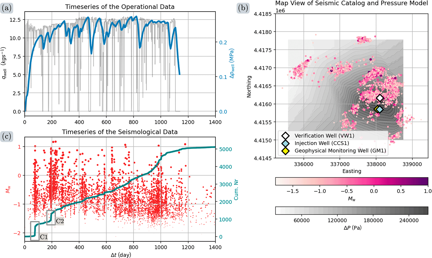
Figure 9. Arrangement of the input data for our model from the IBDP.
(a) Hydraulic data
and
over the 1100 day duration of the project. We use the differential pressure at
from the pressure model of Luu et al. (2022).69 (b) Map of the injection site including the injection well CCS1 (blue), the verification well VW1 (white), the geophysical monitoring well GM1 (yellow), the spatial distribution of
(pink to purple), and the fluid overpressure
ranging from
(white) to
(dark gray). (c) Temporal evolution of seismic event moment magnitudes
(red) and the cumulative number of seismic events
(teal). Two seismic clusters of interests are highlighted with inset boxes labeled C1 and C2 (adapted with data from Dando et al. (2021)67 and Luu et al. (2022)69).
Ethics and consent
Ethical approval and consent were not required.









