Introduction
The principal aim of the present investigation is to design and evaluate a deep learning algorithm, compliant with the HL7 FHIR standard,1,2 for the automatic detection of aortic calcification on chest radiographs obtained at the Fondazione Toscana Gabriele Monasterio (FTGM). Identifying aortic arch calcification (AAC) on chest X-rays is a valuable tool for diagnostic and risk stratification purposes.
This research represents a direct continuation and application of our previous work focused on developing robust methodologies for healthcare interoperability and standardization.3–9 Hashimoto et al.10 demonstrated that AAC severity on chest radiographs correlates positively with abdominal aortic calcification measured by lumbar spine lateral radiography and CT. Furthermore, Komatsu et al. and Lee et al.11 independently found that AAC progression is significantly associated with both cardiovascular and all-cause mortality in high-risk populations, such as hemodialysis patients. Additionally, AAC severity is markedly higher in patients with diabetes or renal dysfunction, correlating with the clustering of atherosclerotic risk factors.
Early detection of AAC through chest radiography can help in atherosclerotic risk stratification. Since chest radiographs are a routine imaging examination, detecting AAC in these images can provide valuable information for atherosclerotic risk stratification. This can help physicians identify patients who might benefit from early interventions to reduce their risk of cardiovascular events.
In summary, detecting AAC on chest radiographs can help physicians to:
• Assess the extent of calcification in the aorta.
• Identify patients at high risk of cardiovascular diseases.
• Implement early interventions for risk factor management.
Cardiovascular diseases are a leading cause of morbidity and mortality worldwide, with aortic calcification being a common indicator of these conditions.12 Accurately detecting calcification using medical imaging techniques is crucial for early diagnosis and effective treatment. Recent advancements in artificial intelligence, particularly in the field of deep learning, have opened up new possibilities for enhancing the analysis of aortic calcification in DICOM images.13,14
Moreover, it is crucial to detect aortic calcification, including in images not originally acquired for this purpose. This method can help identify calcification as soon as the images are acquired from the imaging modality. Several studies have explored the use of AI, specifically convolutional neural networks, to assist radiologists and physicians in the detection and quantification of aortic calcification.15
This research investigates the potential of utilizing convolutional neural networks to assist radiologists and physicians in the identification of aortic calcification. The proposed method aims to improve qualitative assessment of calcification, ultimately contributing to improved patient outcomes.
The dataset employed in this study comprises DICOM studies from our hospital, Gabriele Monasterio Foundation, featuring a diverse range of manually and LLM-annotated calcification patterns, which proved invaluable in training and validating the deep learning model, enabling it to exhibit high levels of precision and recall in detecting the presence of calcification. The LLM annotation was made on X-ray reports associated with DICOM chest X-ray images used in the study.
Aortic calcification is a significant marker for cardiovascular diseases, often detected through imaging techniques such as X-rays. The use of neural network models has shown promising results in automating the detection and classification of aortic calcification, improving diagnostic accuracy and efficiency.
Convolutional neural networks
1.
DenseNet: This model, characterized by dense connections between its layers, has been widely used for medical image classification. In,1 a network combining EfficientNetB0 [10] and DenseNet121 [11], enhanced by attention mechanisms, is presented for precise pneumonia image classification. Other configurations, such as DenseNet169 and DenseNet201 [11], have been used in various studies for detecting pathologies from chest X-rays. The family of DenseNet models leverages strong inter-layer connectivity, promoting feature reuse and reducing the risk of overfitting. DenseNet121 and DenseNet169 have shown particularly robust performance in medical imaging, especially for detecting calcifications.
2.
ResNet: Known for its architecture with residual blocks, ResNet has been used in several studies for medical image classification. ResNet50 is one of the most popular variants, employed in studies like14 for detecting aortic stenosis and in16 for lung disease classification. ResNet50 and its variants have been widely used in medical image analysis, including the detection of aortic calcification, due to their ability to handle complex patterns in imaging data.
3.
Inception: This model, based on the idea of using convolutional filters of different sizes to capture features at multiple scales, has been successfully used for medical image classification. InceptionV3 is a popular variant, employed in17 for pneumonia detection and in14 for detecting aortic stenosis. InceptionV3 has been employed in ensemble models to enhance the detection accuracy of aortic calcification in X-ray images.
4.
VGG: VGG16 and VGG19 are convolutional neural network (CNN) architectures developed by the Visual Geometry Group (VGG) at the University of Oxford. These models are renowned for their depth and simplicity, making them highly effective for image classification tasks. VGG1616,18,19 comprises 16 weight layers, including 13 convolutional layers and 3 fully connected layers. It processes images through a series of convolutional layers with small receptive fields (3x3 filters), followed by max-pooling layers, and finally fully connected layers. The depth of VGG16 allows it to capture intricate features from input images, making it suitable for various image analysis tasks. VGG1920,21 consists of 19 weight layers, with 16 convolutional layers and 3 fully connected layers. The additional convolutional layers in VGG19 enable it to extract more complex features from images, enhancing its performance in detailed image analysis. These architectures are often integrated with other models or employed in ensemble methods to improve the accuracy of medical image classification.
5.
MobileNet: Designed for mobile devices, MobileNet is a family of lightweight and fast models suitable for applications with limited resources. MobileNetV2 has been used in18,19 for pneumonia detection.
Ensemble Models: Several studies have shown that using an ensemble of models, combining the predictions of different individual models, can improve the accuracy and robustness of diagnosis. For example, in,9 an ensemble of InceptionV3, ResNet50, and DenseNet121 achieved the best performance for detecting aortic stenosis. In19 an ensemble of DenseNet169, MobileNetV2, and Vision Transformer (ViT) improved accuracy in pneumonia detection.
Research objectives
The primary objectives of this research are (1) to develop and validate a deep learning model for automated detection of aortic arch calcification in chest radiographs; (2) to evaluate model performance using rigorous cross-validation methodology; (3) to implement the model within a FHIR-compliant workflow ensuring healthcare system interoperability; and (4) to assess feasibility for clinical integration. Secondary objectives include evaluating transfer learning utility and quantifying computational requirements for clinical deployment.
The role of AI in medical imaging
Advancements in artificial intelligence (AI), particularly through deep learning algorithms, are revolutionizing the analysis of medical imaging, especially in identifying conditions like aortic calcification. These algorithms enhance the precision and efficiency of image interpretation, enabling healthcare professionals to detect subtle changes that may indicate disease progression. For instance, deep learning models can automatically segment and quantify abdominal aortic calcification from lateral lumbar radiographs, providing critical insights into patient prognosis.22 This capability is particularly significant given that abdominal aortic calcification severity serves as an independent predictor of cardiovascular events and mortality, especially in high-risk populations such as patients with chronic kidney disease. By integrating deep learning techniques in clinical settings, radiologists can achieve a higher accuracy in quantifying calcification severity compared to traditional methods. This not only aids in early diagnosis but also facilitates more personalized treatment planning. Moreover, the use of these advanced algorithms allows for the analysis of large datasets, improving the understanding of the relationship between calcification and various cardiovascular diseases. As AI continues to evolve, its role in improving diagnostic imaging will likely expand, underscoring the need for ongoing research and development in this area to harness the full potential of technology in enhancing patient care.
Background of aortic calcification
Aortic calcification is a pathological process characterized by the deposition of calcium salts in the aortic valve and vascular structures, significantly impacting cardiovascular health. This condition is not merely a benign finding; it is increasingly recognized as a critical contributor to cardiovascular morbidity and mortality. Calcific aortic valve disease (CAVD) is particularly alarming, with its prevalence on the rise due to aging populations, lifestyle factors, and underlying diseases such as diabetes and hypertension. The mechanism of CAVD involves complex interactions between valvular cells that exhibit osteogenic and fibrogenic activities, leading to fibrocalcification. The use of deep learning algorithms, particularly convolutional neural networks, has the potential to automate the analysis of aortic calcification in medical imaging, reducing the time required for diagnosis and improving the level of consistency in the detection of calcification.
Materials and methods
Dataset Acquisition: The study utilized a consolidated dataset of 1,963 images, resulting in a near-balanced class distribution of 51.45% positive cases and 48.55% negative cases. The positive class consists of 1,010 Anterior-Posterior (AP) chest X-ray images, derived from CT scans. These images were extracted from original CT scans with a diagnosis of aortic calcification, while the negative class comprises 953 normal chest X-ray images similarly derived from CT scans. All images were obtained from the institution’s Picture Archiving and Communication System (PACS).
Ethical Considerations and Informed Consent: This study was conducted in accordance with the Declaration of Helsinki and was approved by the institutional ethics committee (Comitato Etico Regione Toscana - Area Vasta Nord Ovest, protocol number 26533). Informed consent for participation in research was obtained from all subjects involved in the study. Specifically, all participants provided written informed consent at the time of their clinical examination, which included authorization for the retrospective use of de-identified clinical data and images for scientific research and quality assurance purposes. The study exclusively included adult participants; therefore, minor assent was not required.
Annotation Strategy: For the institutional dataset, ground truth labels were generated by analyzing the associated radiological reports using a Large Language Model (Gemma2) to identify documented calcifications, followed by manual validation.
We first evaluated the model on a classic random train→validation→test split to obtain single-run metrics directly comparable to related literature. To assess robustness and eliminate the risk of accidental bias due to a particular data partition, we additionally performed stratified k-fold cross-validation as recommended for reliable machine learning model reporting. K-fold cross-validation
is a widely used statistical technique in machine learning for assessing the generalizability and robustness of predictive models. In this method, the original dataset is randomly partitioned into ‘k’ equal-sized subsets, known as folds. During each of k iterations, one fold is designated as the validation set for testing the model, while the remaining k − 1 folds are used for training. This process is repeated until each fold has served once as the validation set. The model’s performance is then evaluated by averaging the results across all folds, providing an unbiased estimate of its generalization ability. K-fold cross-validation helps to mitigate the risk of overfitting that can arise from relying on a single train/test split and is particularly valuable when working with limited or imbalanced data. Typically, the value of k is chosen as 5 or 10, but it can be adjusted based on dataset characteristics and computational resources. This approach is considered a best practice for model evaluation in biomedical machine learning applications.23
Preprocessing pipeline
The CT DICOM images were preprocessed using a dedicated pipeline to remove those containing pacemakers or other artifacts that could negatively impact the training phase. The pipeline is composed of several steps.
1.
DICOM to JPG Conversion: DICOM files were converted to JPG format using offis dcmtk24 to facilitate image handling and take into account the various DICOM transfer syntaxes due to the differences in formats of the two X-ray modalities present in our institute.
2.
Lung Segmentation: A publicly available pre-trained lung segmentation algorithm publicly available25 was employed to crop the images to the region of interest, the thorax, reducing the computational complexity of the model for the subsequent model training.
3.
Resizing: Images were resized to a uniform size of 400x400 pixels using bilinear interpolation to ensure compatibility with the deep learning model.
4.
Normalization: Pixel values were normalized to the range of [0, 1] by dividing each pixel value by 255 to improve the model’s performance.
5.
Array Conversion: The processed images were converted into an array to be used as input for the subsequent phase of the model. The model was developed using TensorFlow and Keras in Python 3.
An overview of the DICOM image preprocess is presented in
Figure 1.
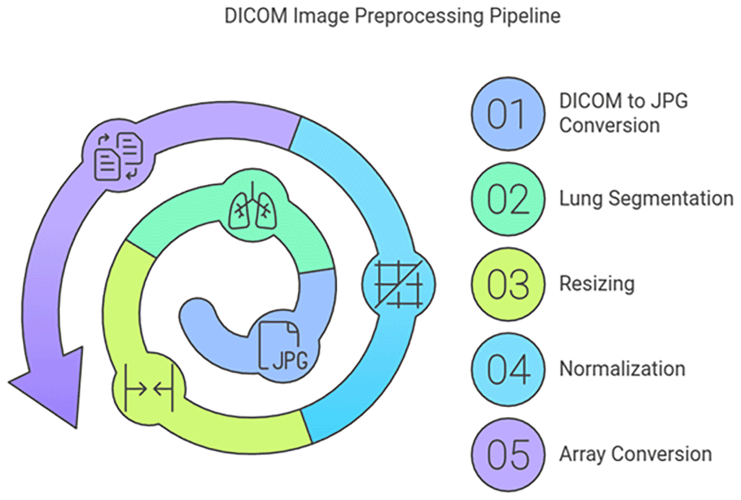
Figure 1. DICOM preprocessing image pipeline.
The dataset was randomly divided into training, validation, and test subsets using a two-stage stratified random sampling approach. In Stage 1, the complete dataset was partitioned 80/20 into training and test subsets: the training set included 1,570 images, and the test set included 393 images. In Stage 2, the training set was further divided into training-only (90%, 1,413 images) and validation (10%, 157 images) subsets to ensure proper evaluation without contamination. The chest X-ray image dataset, sourced from our institution’s Picture Archiving and Communication System (PACS), consists of 1,010 images with a diagnosis of aortic calcification and 953 normal images.
The final consolidated dataset comprised 1963 images, resulting in a near-balanced class distribution of 51.45% positive cases and 48.55% negative cases. This favorable balance reduces the need for aggressive class-weight adjustments and minimizes the risk of model bias toward the majority class. Additionally, the images were resized to a common size of 400x400x3 to adhere to the framework’s requirements. After normalization, the pixel values across all images were represented as array data. After normalization in the range [0,1] for every pixel in an image, array data representation of all the images is constructed. After that, data augmentation was applied – exclusively to the training set (1,570 images) – during model training to simulate real-world acquisition variability. The data augmentation process employs an ONLINE strategy via Keras ImageDataGenerator.flow() with batch processing (batch_size = 20), applying random transformations to each image during each training epoch. This approach generates novel variants dynamically rather than pre-generating and storing augmented images, providing memory efficiency while maintaining high augmentation diversity.
The augmentation pipeline consists of five sequential transformation steps, each applied stochastically during training:
•
Rotation (rotation_range = 30): Simulates patient positioning variance during X-ray acquisition (±30° range, continuous distribution)
•
Zoom (zoom_range = 0.2): Represents variation in patient distance from X-ray source (80%–120% range, simulating 0.8–1.2× magnification)
•
Horizontal Shift (width_shift_range = 0.1): Represents horizontal patient positioning variance (±10% of image width)
•
Vertical Shift (height_shift_range = 0.1): Represents vertical patient positioning variance (±10% of image height)
•
Horizontal Flip (horizontal_flip = True): Ensures model invariance to PA (posteroanterior) vs AP (anteroposterior) chest projection
Note: Vertical flip was explicitly disabled (vertical_flip = False) as it is clinically inappropriate for radiographic anatomy.
An overview of the image data augmentation process is presented in
Figure 2.
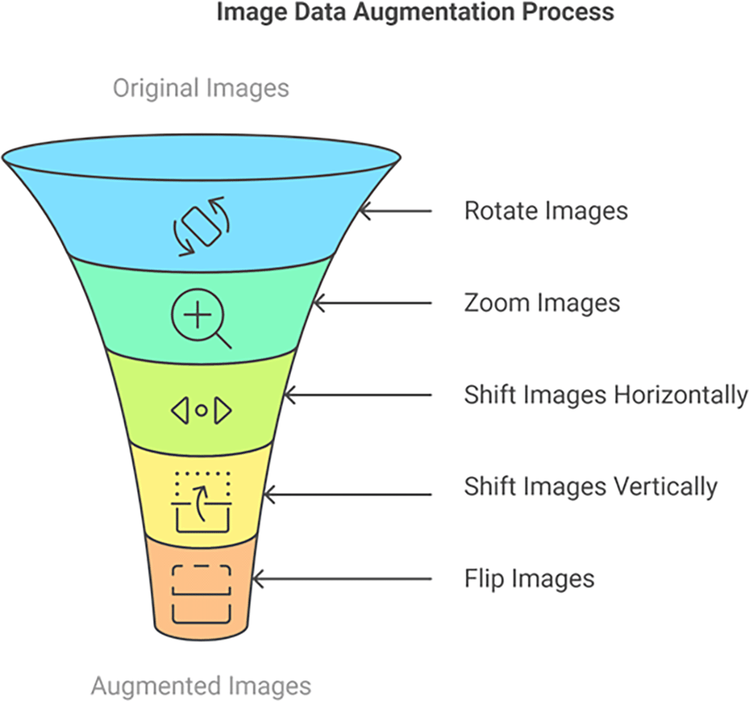
Figure 2. Online image data augmentation pipeline for training set.
Data augmentation is used in deep learning, and particularly in image classification, for several crucial reasons:
1. Increase Dataset Size: Deep learning models, especially complex ones like CNNs, require vast amounts of data to train effectively. Collecting and labeling a large, diverse dataset of medical images can be expensive, time-consuming, and sometimes impractical. Data augmentation artificially expands the training dataset by creating modified versions of existing images. This provides the model with more examples to learn from without the need for collecting new data.
2. Improve Model Generalization and Robustness: A model trained on a limited dataset might overfit to the specific characteristics of that dataset. This means it performs well on the training data but poorly on new, unseen images that differ slightly (e.g., different lighting, orientation, or minor variations in the anatomy). Data augmentation exposes the model to a wider variety of image variations during training. By seeing images rotated, zoomed, shifted, and flipped, the model learns to recognize the underlying features of, say, aortic calcification, regardless of these variations. This makes the model more robust and able to generalize better to new, unseen data. It learns to be invariant to transformations that don’t affect the underlying pathology.
3. Reduce Overfitting: Overfitting occurs when a model becomes too specialized to the training data, memorizing it rather than learning the general patterns. This leads to poor performance on new data. By increasing the diversity of the training data, data augmentation acts as a form of regularization. It helps prevent the model from becoming too reliant on specific features or noise present only in the original training images.
4. Simulate Real-World Variability: Real-world medical images are rarely perfectly standardized. There can be variations in patient positioning, image acquisition parameters, and natural anatomical differences. Data augmentation can simulate these real-world variations, making the model more adaptable to the kind of images it will encounter in a clinical setting. For instance, slight rotations can mimic variations in patient positioning during an X-ray.
An overview of the entire image classification process is presented in
Figure 3. In the specific problem of detecting aortic calcification in chest X-rays, data augmentation is valuable because:
1. Calcifications can appear in slightly different locations, orientations, and sizes. Augmentations like rotation, shift, and zoom help the model learn to recognize calcifications regardless of these variations.
2. X-rays can be taken at slightly different angles or with minor variations in patient positioning. Rotation and shift augmentations help simulate these variations.
3. We have a dataset of 1010 images for the calcification class. While this is a decent number, it might still be limited for training a complex CNN from scratch. Augmentation helps us make the most of this data.
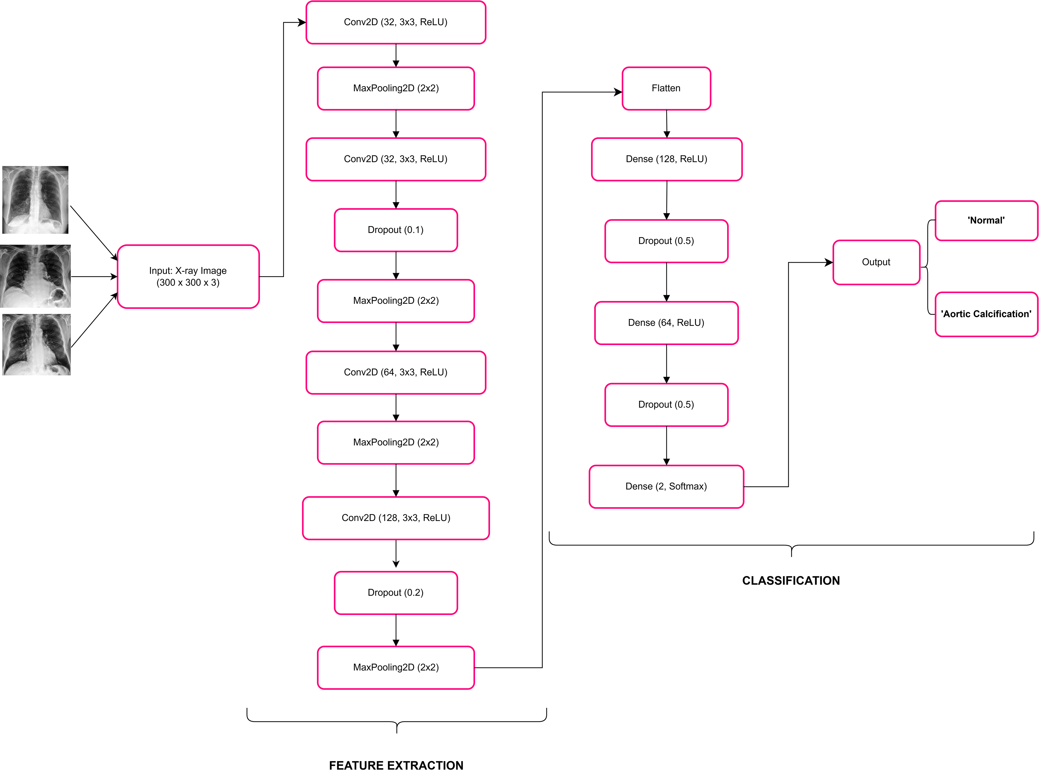
Figure 3. Example of image classification process.
Figure 4 illustrates the layer-by-layer structure of the CNN model utilized in this research. The layers of a CNN act as the fundamental building blocks of these models. When a filter is applied to an input, it produces an activation, which is the core process of convolution. By repeatedly applying the same filter to the same input, a feature map is generated. This map highlights the locations and intensities of a detected pattern within the input, effectively creating an image of the pattern. Another crucial component of a CNN architecture is the pooling layer. The pooling layer reduces the dimensions of the feature sets, thereby decreasing the number of parameters to learn and the computational load of the network. It aggregates the features within a feature map created by a convolution layer over a specific region. A further important layer is the dropout layer: a dropout layer in a convolutional neural network (CNN) for image classification is used to prevent overfitting. Overfitting occurs when a model performs well on training data but poorly on unseen test data. The Dropout layer helps mitigate this by randomly setting a fraction of input units to zero during training, which in this case is 50% (0.5). This forces the network to learn more robust features and reduces the reliance on specific neurons, thereby improving the model’s generalization to new data.
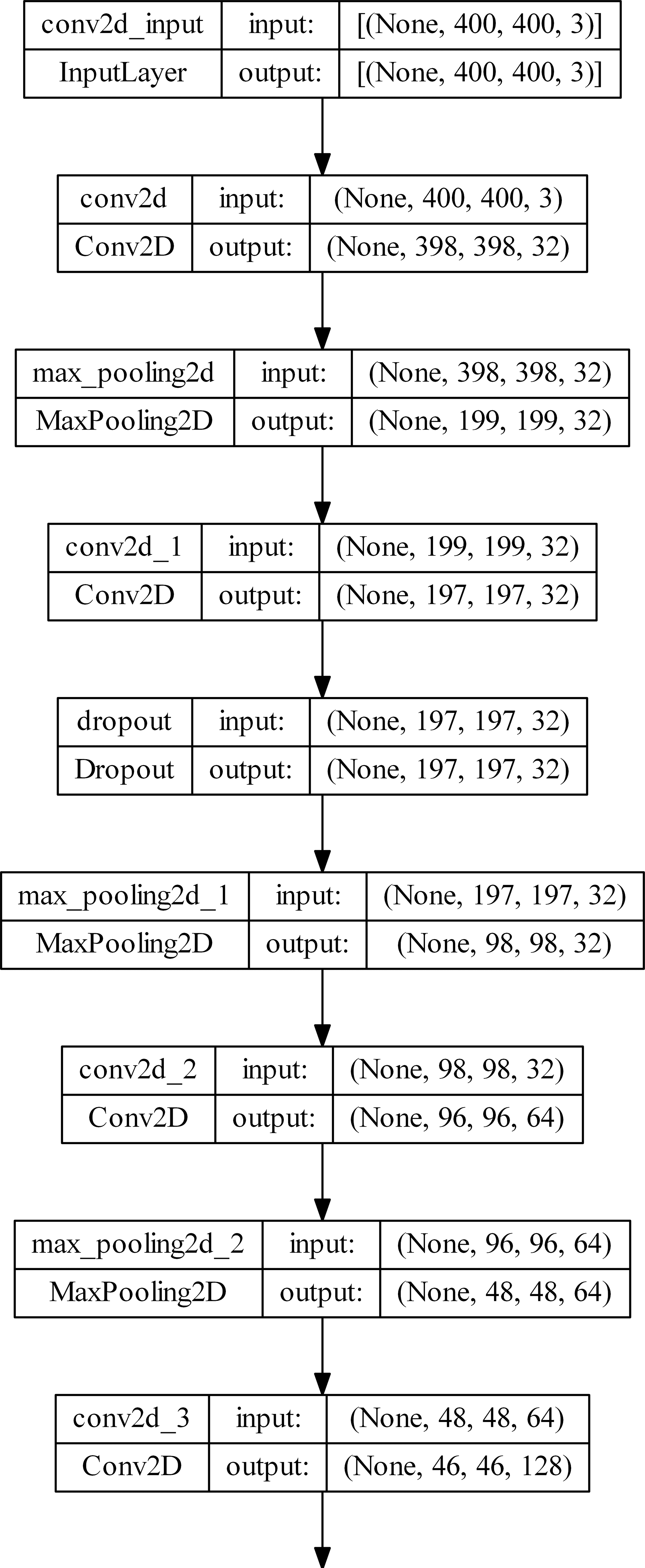
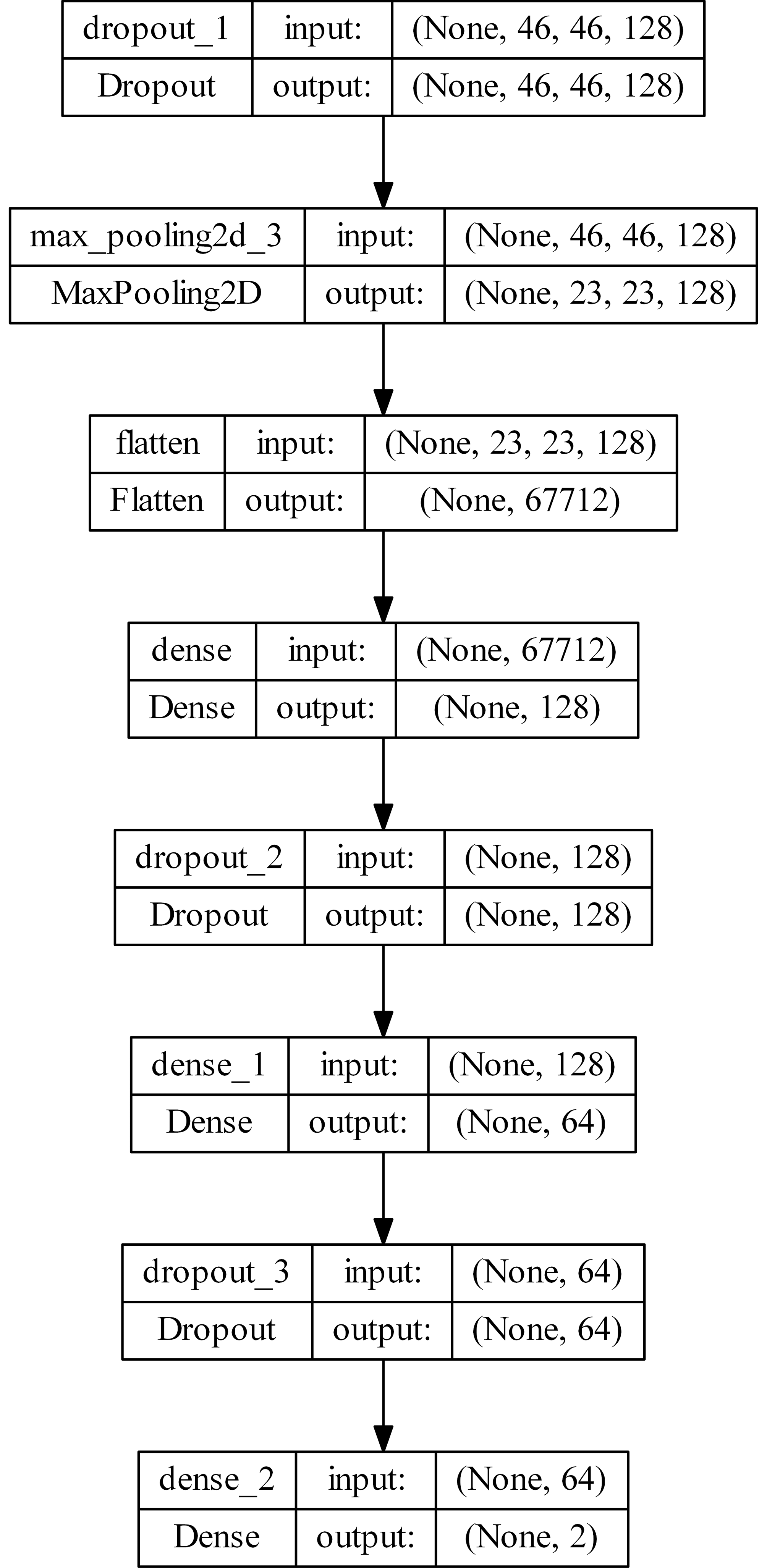
Figure 4. Layer-by-Layer architecture of the proposed Convolutional Neural Network (CNN) model.
Dropout acts as a regularization technique that enhances the model’s ability to generalize by preventing it from becoming too dependent on particular neurons. This leads to a more resilient and effective model for image classification tasks.
Each 2DConv layer is followed by the activation layer with the ReLU activation function. The Rectified Linear Unit (ReLU) activation function is widely used in neural networks, particularly in Convolutional Neural Networks (CNNs). It is mathematically expressed as:
It passes the input value directly if it is positive; otherwise, it outputs zero. This function adds non-linearity to the model while maintaining computational efficiency.
The total number of parameters is 8,778,146; trainable params: 8,778,146; non-trainable params: 0.
The model completed training with an early stopping mechanism. Early stopping halted training when validation accuracy plateaued for 5 epochs, restoring the best weights from the training run. The learning rate was reduced by a factor of 0.2 whenever validation loss plateaued for 5 epochs.
Training settings
• Optimizer: Adam, learning rate 0.001
• Loss: categorical cross-entropy
• Batch size: 20
• Epochs: up to 100 (early stopping when validation accuracy plateaued for 5 epochs)
• Learning rate adjustment: ReduceLROnPlateau (factor 0.2, patience 5)
• Data augmentation (training set): rotation_range = 30°, zoom_range = 0.2, width_shift_range = 0.1, height_shift_range = 0.1, horizontal_flip = True, vertical_flip = False
• Validation: Stratified 5-fold cross-validation
• Total parameters: 8,778,146
Training progress at key milestones
Table 1 shows the training metrics at critical points during the 100-epoch training process.
Table 1. Training performance metrics at key epochs.
| Epoch | Train accuracy (%) | Train loss | Val accuracy (%) |
Val loss |
|---|
| 1 | 66.88 | 0.6012 | 94.27 | 0.2651 |
| 10 | 97.03 | 0.0928 | 97.45 | 0.0900 |
| 25 | 97.88 | 0.0732 | 97.45 | 0.0852 |
| 50 | 97.81 | 0.0737 | 97.45 | 0.0851 |
| 75 | 97.52 | 0.0773 | 97.45 | 0.0851 |
| 100 | 97.95 | 0.0666 | 97.45 | 0.0851 |
Training statistics summary
Table 2 provides a consolidated summary of the training and validation performance statistics.
Table 2. Summary of training and validation performance statistics.
| Metric |
Value |
|---|
| Train Accuracy (Min) | 66.88% at Epoch 1 |
| Train Accuracy (Max) | 98.37% at Epoch 32 |
| Train Accuracy (Final) | 97.95% |
| Val Accuracy (Min) | 93.63% at Epoch 5 |
| Val Accuracy (Max) | 98.09% at Epoch 6 |
| Val Accuracy (Final) | 97.45% |
| Best Epoch | Epoch 6 (98.09%) |
| Train Loss (Max) | 0.6012 at Epoch 1 |
| Train Loss (Min) | 0.0561 at Epoch 22 |
| Train Loss (Final) | 0.0666 |
| Val Loss (Max) | 0.2651 at Epoch 1 |
| Val Loss (Min) | 0.0779 at Epoch 9 |
| Val Loss (Final) | 0.0851 |
Key observations
•
Rapid Convergence: The model achieved 97.45% validation accuracy by epoch 10, demonstrating fast convergence to optimal performance.
•
Peak Performance: The Best validation accuracy of 98.09% was reached at epoch 6, followed by stable performance through epoch 100.
•
Stability: From epoch 8 onwards, validation accuracy stabilized at approximately 97.45%, indicating the model has converged and no overfitting is occurring.
•
Final Performance: At epoch 100, the model maintains 97.45% validation accuracy with a loss of 0.0851, confirming consistent performance throughout training.
•
Training Efficiency: The model achieves near-peak validation accuracy in just 10 epochs, making it highly efficient for resource-constrained scenarios.
•
No Overfitting: Final train accuracy (97.95%) and validation accuracy (97.45%) are well-aligned, indicating good generalization.
A visual representation of the model’s training and validation progress, confirming the stability and rapid convergence, is provided in
Figure 5.
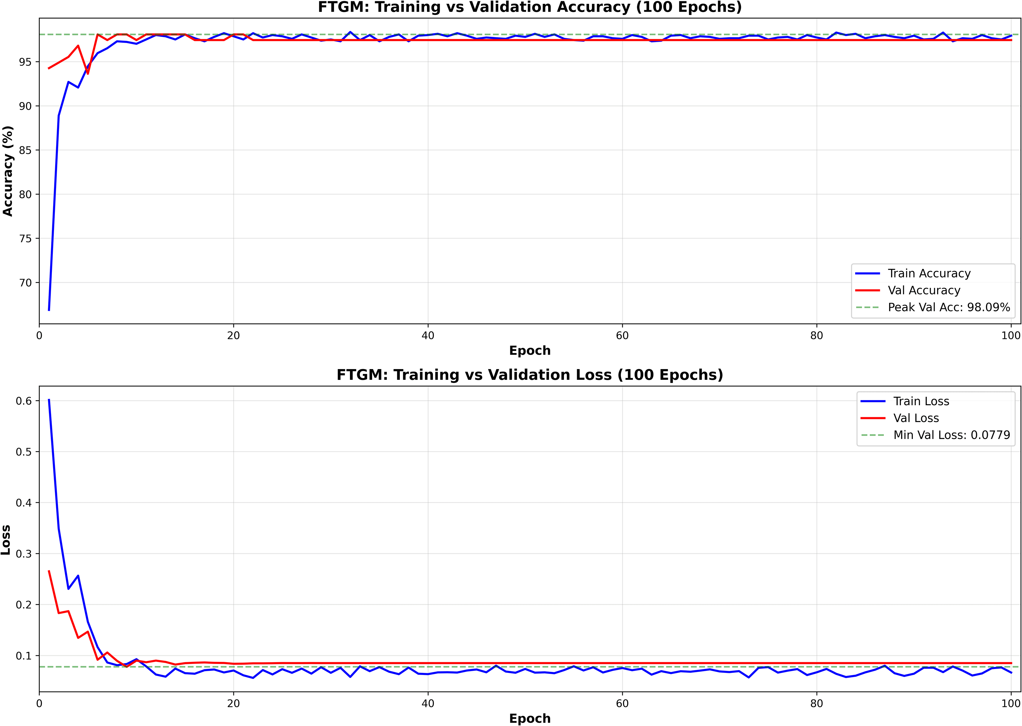
Figure 5. Visual representation of training and validation accuracy/loss over epochs.
Only pixel rescaling (1/255) was applied to validation and test sets. No geometric transformations (rotation, zoom, shift, or flip) were applied to maintain uncontaminated evaluation conditions.
Loss and Accuracy on test Dataset:
25/25 [==============================] - 7 s 280 ms/step - loss: 0.0851 - acc: 0.9771.
Test Set Results:
- Test Accuracy: 0.9771 (97.71%)
- Test Loss: 0.0851
- Batch processing: 25/25 batches completed
- Processing time: 7 seconds, 280 milliseconds per batch
Random prediction
Examples of predictions made by the trained model on randomly selected images from the dataset.
Figure 6 presents sample chest X-ray images predicted by the model on the test dataset.
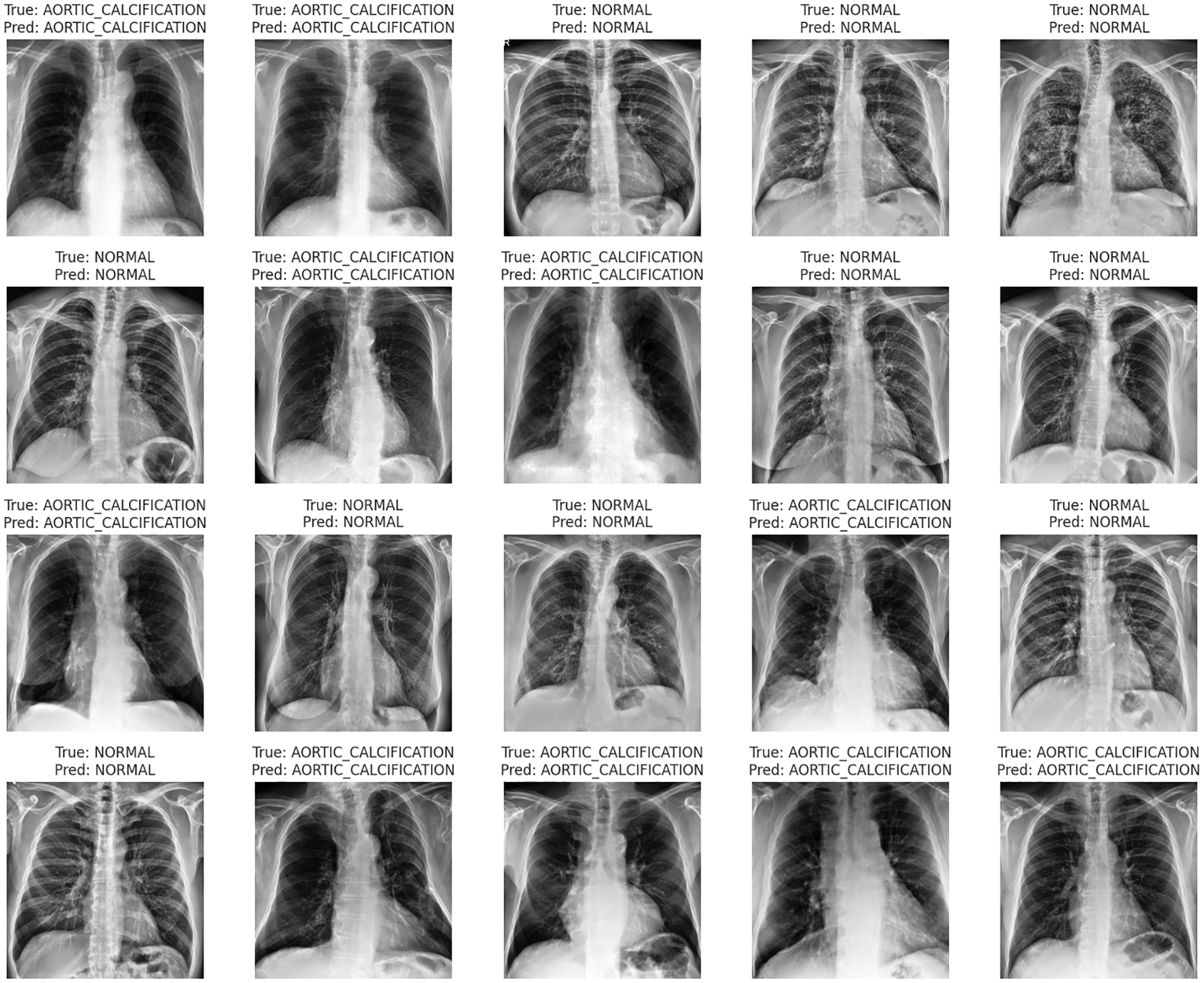
Figure 6. Examples of predicted chest X-ray images from the test dataset.
Classification Report by Class:
Class 0 (NORMAL):
- Precision: 0.9780
- Recall: 0.9727
- F1-Score: 0.9753
- Support: 183
Class 1 (AORTIC_CALCIFICATION):
- Precision: 0.9763
- Recall: 0.9810
- F1-Score: 0.9786
- Support: 210
Overall Metrics:
- Macro Average Precision: 0.9772
- Macro Average Recall: 0.9768
- Macro Average F1-Score: 0.9770
- Total Test Samples: 393
The final classification metrics for the test set, including macro averages for Precision, Recall, and F1-Score, are visually summarized in
Figure 7.
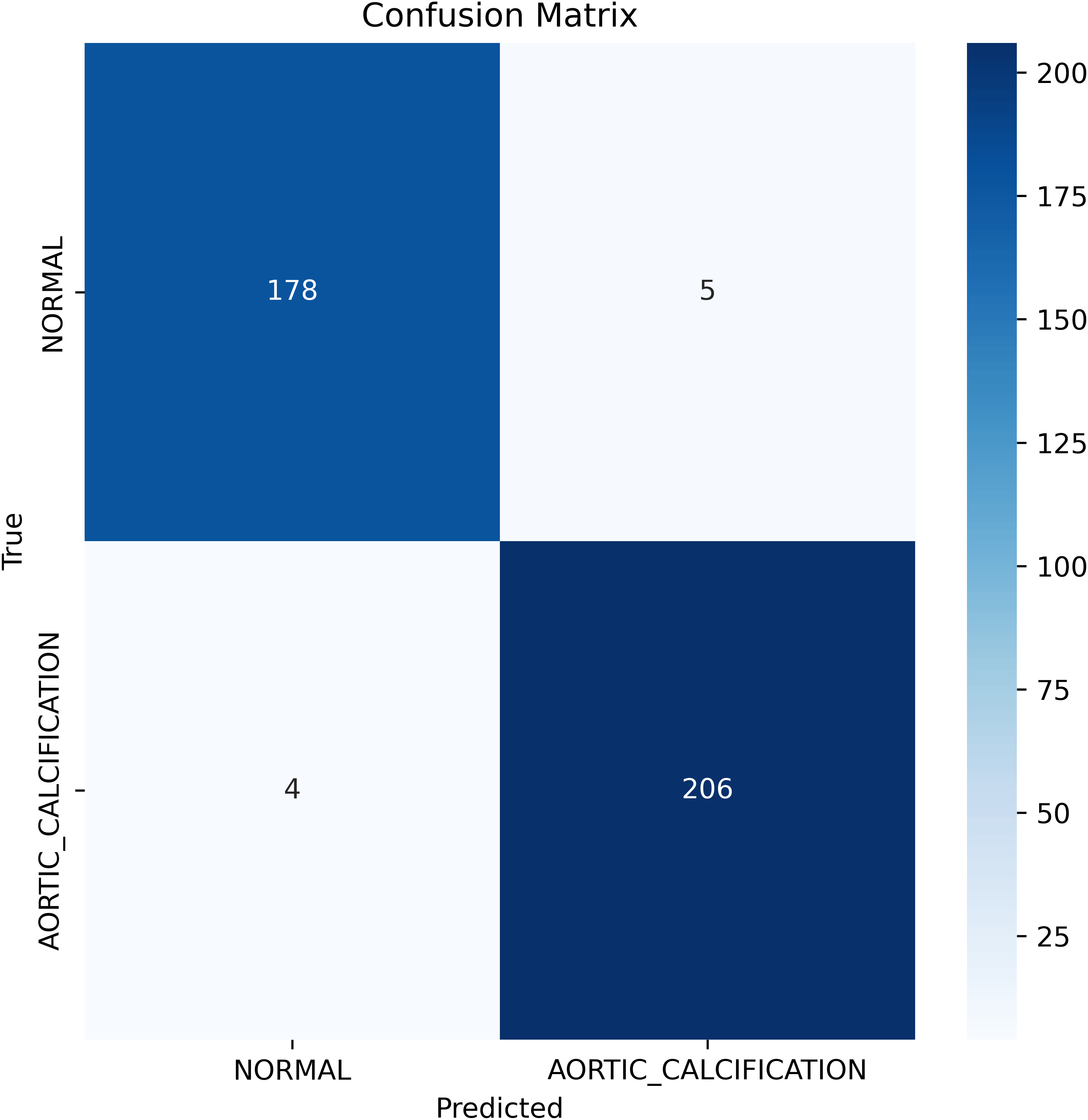
Figure 7. Visual representation of classification report metrics.
Results were consistent across k-fold cross-validation (
Table 3), with a mean validation accuracy of 0.9679 (SD 0.0282), mean validation loss of 0.0778 (SD 0.0581), and mean AUC-ROC of 0.9990 (SD 0.0006), demonstrating the model’s stability regardless of partitioning. Stratified five-fold cross-validation was performed to assess robustness and generalizability. For each fold, model performance metrics included accuracy, sensitivity, specificity, precision, F1-score, and AUC-ROC, with summary statistics reported across folds.
Table 3. Stratified 5-fold cross-validation performance metrics.
| Fold | Validation accuracy | Validation loss | AUC-ROC
| Confusion matrix |
|---|
| 1 | 0.989821 | 0.044888 | 0.999248 |
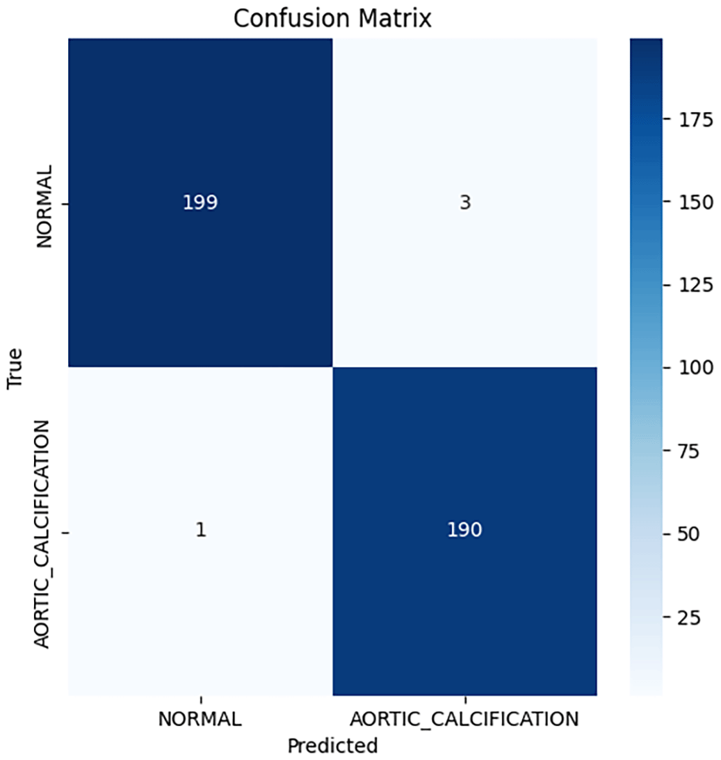
Figure 8. confusion matrix for stratified 5-fold cross-validation, fold 1. |
| 2 | 0.987277 | 0.071250 | 0.998911 |
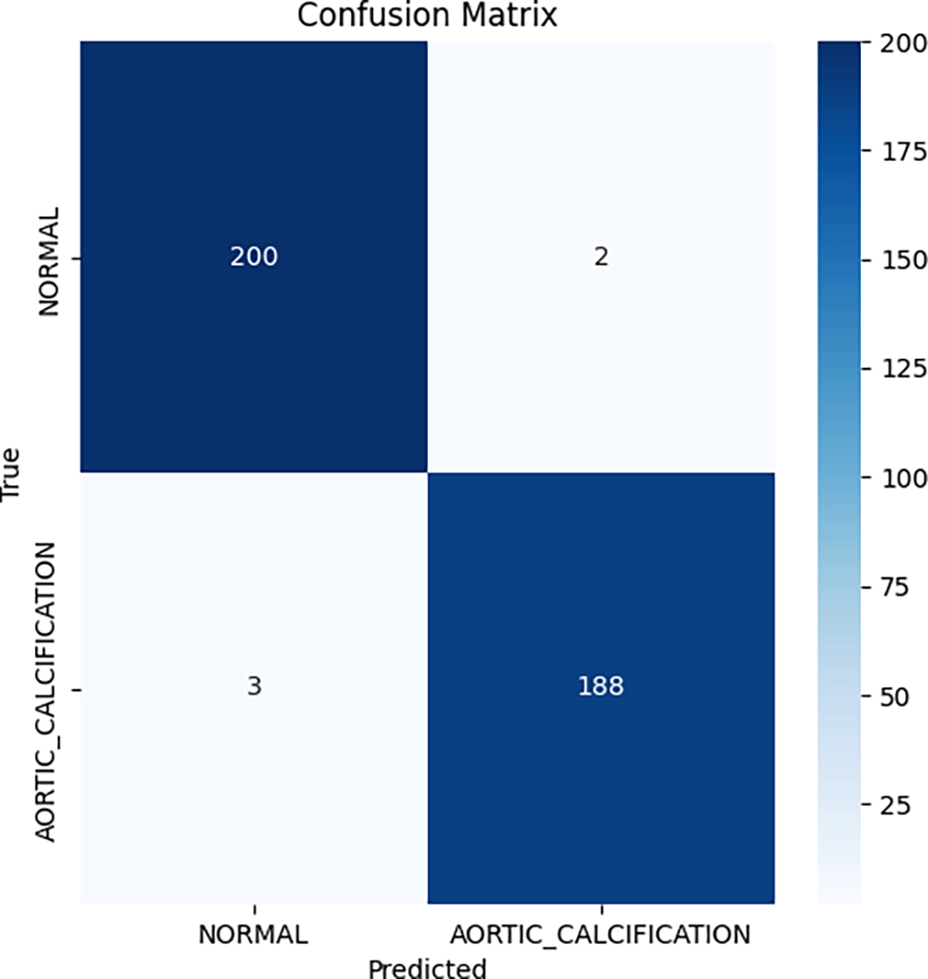
Figure 9. Confusion matrix for stratified 5-fold cross-validation, fold 2. |
| 3 | 0.987277 | 0.057077 | 0.999637 |
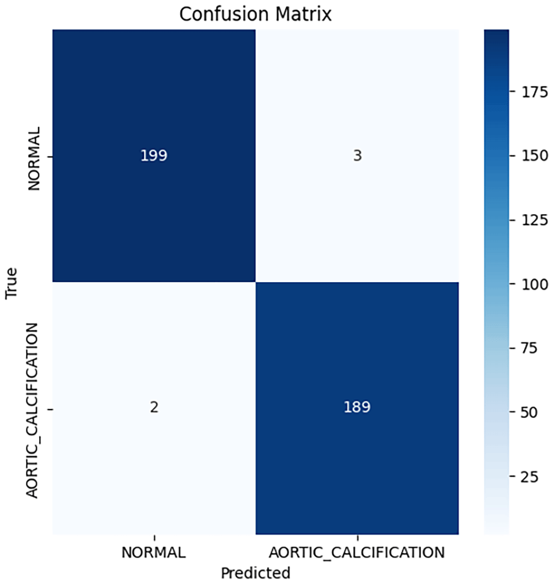
Figure 10. Confusion matrix for stratified 5-fold cross-validation, fold 3. |
| 4 | 0.989795 | 0.064343 | 0.998097 |
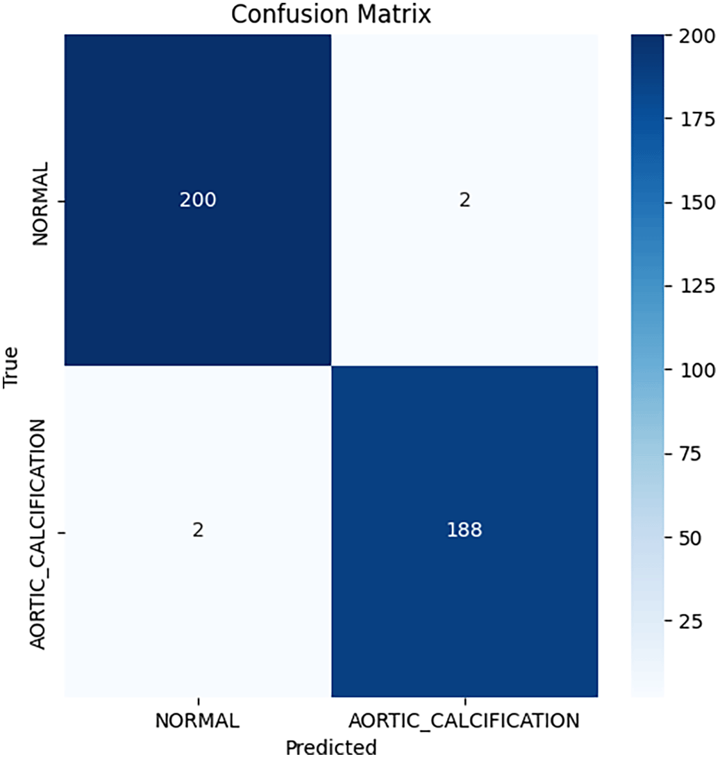
Figure 11. Confusion matrix for stratified 5-fold cross-validation, fold 4. |
| 5 | 0.989795 | 0.033726 | 0.999088 |
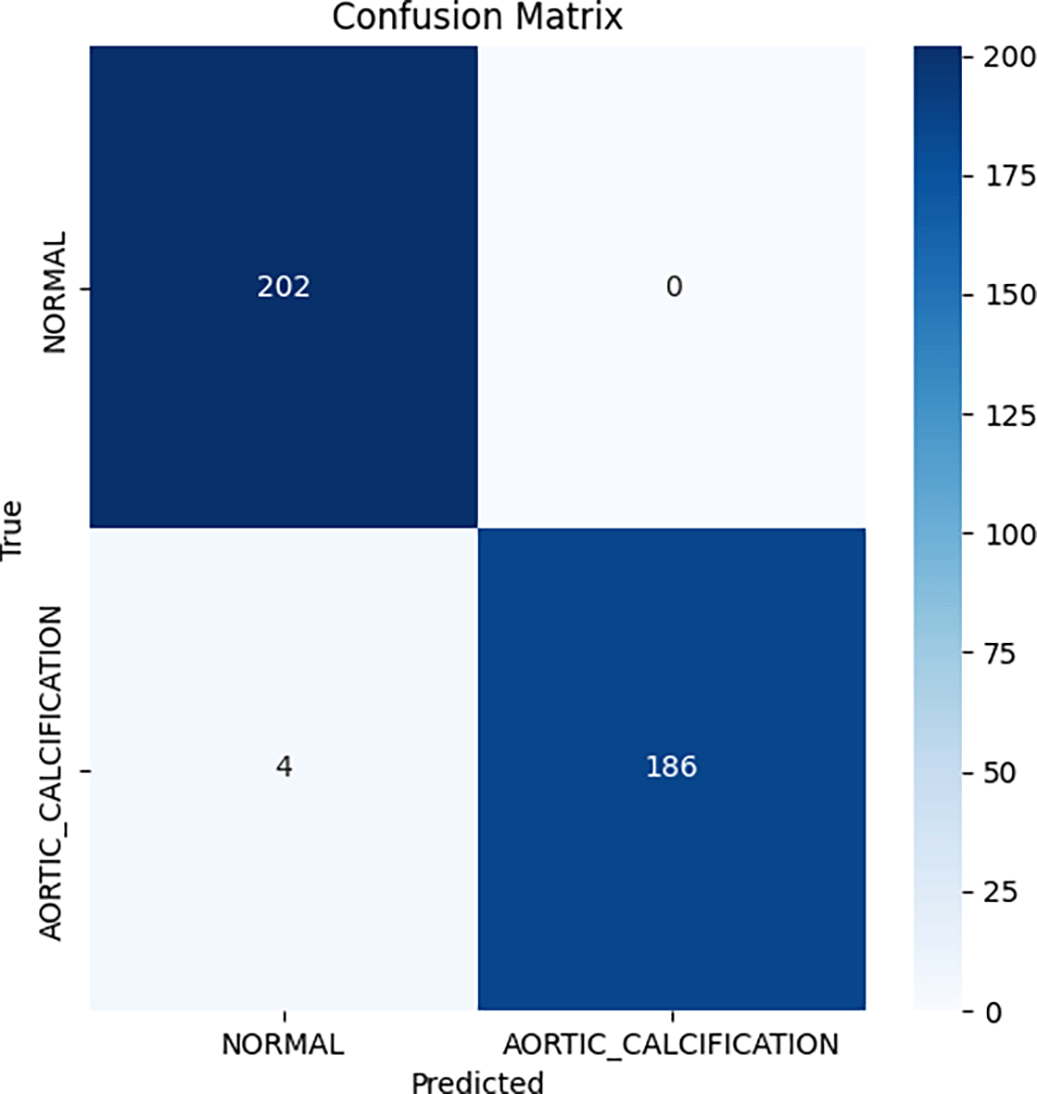
Figure 12. Confusion matrix for stratified 5-fold cross-validation, fold 5. |
| Mean ± SD
| 0.9888 ± 0.0012
| 0.0543 ± 0.0135
| 0.9990 ± 0.0005
| --
|
Reporting both the single split and k-fold cross-validation performance (
Table 4) enabled direct benchmarking with previous studies while also demonstrating that our model’s high performance was not the product of a favorable split but rather persisted across multiple partitions of the data. The minimal variance across folds supports the robustness and applicability of the method to broader clinical populations.
Table 4. Comparative classification performance metrics of deep learning models on the test dataset.
| Model | Accuracy | Precision | Recall |
F1-score |
|---|
| FTGM single run | 0.9771 | 0.9772 | 0.9768 | 0.9770 |
| K1 | 0.9898 | 0.9897 | 0.9900 | 0.9898 |
| K2 | 0.9873 | 0.9873 | 0.9872 | 0.9873 |
| K3 | 0.9873 | 0.9872 | 0.9873 | 0.9873 |
| K4 | 0.9898 | 0.9898 | 0.9898 | 0.9898 |
| K5 | 0.9898 | 0.9903 | 0.9895 | 0.9898 |
In this research, we utilized the confusion matrix and standard metrics such as accuracy, precision, recall, specificity, and F1-score to evaluate both the pre-trained models and our proposed model. Accuracy is a widely used metric to measure the performance of deep learning models. It represents the ratio of correctly classified samples to the total number of samples, calculated by dividing the sum of true positive and true negative predictions by the total number of predictions.26
•
•
•
•
Where TP represents true positives, TN represents true negatives, FP represents false positives, and FN represents false negatives.
Precision quantifies the ratio of correctly predicted instances of a particular class to the total predictions made for that class. Recall measures the proportion of actual positive instances that are correctly identified, calculated as the number of true positives (TP) divided by the sum of true positives (TP) and false negatives (FN). Specificity assesses the proportion of actual negative instances that are correctly identified, determined by dividing the number of true negatives (TN) by the sum of true negatives (TN) and false positives (FP).
Summary statistics
The Table 5 presents a comprehensive comparison of classification performance metrics (Precision, Recall, F1-Score) across eight deep learning models tested on the cardiac pathology detection task. For each model, three aggregated metrics are reported:
•
Accuracy: Overall correctness of the model on the test set
•
Macro Average: Unweighted mean of metrics across both classes
•
Weighted Average: Weighted mean considering class distribution
Table 5. Comparative classification performance metrics of deep learning models on the test dataset.
| Model | Metric | Precision | Recall | F1-Score |
Support |
|---|
| DenseNet201 | accuracy | 0.9796 | 0.9796 | 0.9796 | 0.9796 |
| DenseNet201 | macro avg | 0.9793 | 0.9799 | 0.9796 | 393 |
| DenseNet201 | weighted avg | 0.9797 | 0.9796 | 0.9797 | 393 |
| FTGM | accuracy | 0.9771 | 0.9771 | 0.9771 | 0.9771 |
| FTGM | macro avg | 0.9772 | 0.9768 | 0.9770 | 393 |
| FTGM | weighted avg | 0.9771 | 0.9771 | 0.9771 | 393 |
| InceptionV3 | accuracy | 0.9847 | 0.9847 | 0.9847 | 0.9847 |
| InceptionV3 | macro avg | 0.9855 | 0.9840 | 0.9846 | 393 |
| InceptionV3 | weighted avg | 0.9849 | 0.9847 | 0.9847 | 393 |
| MobileNetV2 | accuracy | 0.9669 | 0.9669 | 0.9669 | 0.9669 |
| MobileNetV2 | macro avg | 0.9664 | 0.9683 | 0.9669 | 393 |
| MobileNetV2 | weighted avg | 0.9680 | 0.9669 | 0.9670 | 393 |
| NASNetLarge | accuracy | 0.9211 | 0.9211 | 0.9211 | 0.9211 |
| NASNetLarge | macro avg | 0.9230 | 0.9244 | 0.9211 | 393 |
| NASNetLarge | weighted avg | 0.9265 | 0.9211 | 0.9212 | 393 |
| ResNet152V2 | accuracy | 0.9822 | 0.9822 | 0.9822 | 0.9822 |
| ResNet152V2 | macro avg | 0.9820 | 0.9823 | 0.9821 | 393 |
| ResNet152V2 | weighted avg | 0.9822 | 0.9822 | 0.9822 | 393 |
| ResNet50 | accuracy | 0.9389 | 0.9389 | 0.9389 | 0.9389 |
| ResNet50 | macro avg | 0.9399 | 0.9418 | 0.9389 | 393 |
| ResNet50 | weighted avg | 0.9430 | 0.9389 | 0.9390 | 393 |
| VGG19 | accuracy | 0.9644 | 0.9644 | 0.9644 | 0.9644 |
| VGG19 | macro avg | 0.9638 | 0.9649 | 0.9643 | 393 |
| VGG19 | weighted avg | 0.9646 | 0.9644 | 0.9644 | 393 |
All models achieved accuracy above 92%, with InceptionV3 (98.47%) and ResNet152V2 (98.22%) showing the strongest performance. NASNetLarge (92.11%) and ResNet50 (93.89%) showed relatively lower accuracy, while FTGM (97.71%) and DenseNet201 (97.96%) demonstrated competitive performance comparable to more complex architectures.
Standardization and interoperability
Healthcare data fragmentation remains a critical barrier to AI implementation in clinical practice. The HL7 FHIR (Fast Healthcare Interoperability Resources)2 standard provides structured, computable representations of health data, enabling AI algorithms to access diverse data sources (electronic health records, imaging archives, laboratory results) in consistent formats. FHIR compliance ensures portability of this AAC detection model across different hospital systems and healthcare settings, supporting the European Health Data Space (EHDS)27 objective of enabling cross-border health data utilization for research and clinical care.
FHIR integration
The proposed ‘Kinaitics’ workflow implements a pipeline for semantic interoperability. Upon image acquisition, the system ingests the DICOM object and extracts metadata to populate four interlinked FHIR resources: 1. Patient Resource: Stores demographic data to enable age-based risk stratification. 2. ImagingStudy Resource: Preserves the DICOM hierarchy (Study/Series/Instance UIDs) and links to the acquisition modality. 3. Device Resource: Captures technical specifications of the acquisition hardware (e.g., spatial resolution, manufacturer) to track model performance against specific equipment. 4. DiagnosticReport Resource: Encapsulates the AI inference, including probability distributions and confidence scores, formatted according to LOINC and SNOMED CT standards.1,2
FHIR integration: Implementation details
The PACS sends every anteroposterior X-Ray image to the AI model. The pipeline extracts comprehensive metadata from the DICOM image and structures it as FHIR resources within a Bundle construct.
Implementation details of the FHIR-integrated clinical workflow
Overview
The presented FHIR Bundle exemplifies a state-of-the-art approach to digitally capturing the full lineage and auditability of an AI-driven diagnostic event for aortic calcification detection in chest X-ray imaging. This structured collection of FHIR R4 resources ensures compliance with European Electronic Health Record Exchange Format (EEHRxF) and supports semantic interoperability, reproducibility, and future-proof integration within clinical IT systems.
Bundle Structure and Rationale
The bundle is structured as a FHIR “collection” type, encapsulating related resources with internal references via UUIDs (URN scheme). This allows all data—patient demographics, imaging information, acquisition- and inference-device metadata, AI-generated diagnostic output, and complete provenance to be transmitted as a single atomic unit. Doing so ensures both referential integrity and complete traceability, without external server dependencies during transmission or archival.
Resource Composition
1. Patient resource
This entry holds essential demographic information, including patient identifier, name, gender, and date of birth. The identifier schema leverages the DICOM patient-id, ensuring cross-referencing compatibility with imaging modalities and legacy systems. Such demographic data are foundational for risk stratification and compliance with cross-border health data exchange requirements.
2. Imagingstudy resource
The ImagingStudy resource maintains in-depth traceability back to the original DICOM imaging study:
• Identifiers include the DICOM Study Instance UID, Accession Number, and Study ID for seamless PACS linkage.
• Modality is coded via DICOM’s ontology (e.g., “DX” for Digital Radiography), supporting semantic clarity.
• Hierarchical Integrity is preserved across Study, Series, and Instance, each with unique IDs and linked device performer references. This enables precise image retrieval, audit, while the subject reference connects the Study to the correct Patient.
3. Device resources
Two distinct Device resources are included:
• Acquisition Device documents the physical imaging hardware (e.g., FUJIFILM Corporation device, serial number, and software version). Capturing this metadata is essential for AI quality assurance and post-hoc performance analysis, as device variability can impact model accuracy.
• AI (Software) Device represents the computational AI model itself—the inference engine (“FTGM_Aortic_Calc_v1.0_20251014”), treated as a software application in the SNOMED CT ontology. Explicit versioning is a cornerstone for future regulatory compliance, post-market surveillance, and reproducibility.
4. DiagnosticReport Resource
The DiagnosticReport is central to the AI-driven clinical workflow:
• Code and Status: Utilizes LOINC and SNOMED CT for standardized diagnosis encoding and status tracking (“final”).
• Study and Subject Linking: Tightly binds the report to both the originating ImagingStudy and Patient.
• Human-Readable Conclusion and Coded Result: Includes a text summary (e.g., “No acute abnormality detected”) and coded conclusion.
• Expandability: While this instance encodes a normal result, the schema supports richer AI outputs—such as severity scores, class probabilities, and detailed AI-generated observations—using FHIR extensions for transparent, machine-interpretable result sharing.
5. Library resource
This references the source dataset (“MIMIC-CXR-Dataset-v2.0”) used to train the AI model. Including a Library resource adheres to modern model card transparency standards and provides context on data provenance, which is essential for regulatory, ethical, and scientific rigor.
6. Provenance Resource
The Provenance layer weaves together auditability and legal attribution:
• Agent and Entity Structure: Explicitly attributes authorship to the AI software device and connects input ImagingStudy and training data Library via W3C PROV ontology roles (“source”, “instantiates”).
• Timestamping and Targeting: Documents the precise timing of inference and targets the DiagnosticReport, thus locking the event timeline.
• Regulatory Readiness: Fully supports requirements around digital health record keeping, liability, and future EU and FDA AI Act auditing practices.
Implementation and Interoperability Considerations
• Hapi FHIR Library: The conversion from source data to FHIR was implemented in Java using the Hapi FHIR library, which provides robust mechanisms for instantiating, validating, and serializing complex FHIR resources.
• Message Transport: The FHIR Bundle is interoperable with modern orchestration tools (e.g., Nextgen Mirth Connect ESB28), enabling automated dispatch into institutional EHR systems.
• Compliance: The architecture ensures that outputs are EEHRxF and HL7 FHIR-compliant, supporting pan-European data mobility for both direct clinical care and research use cases.
• Audit, Adaptability, and Security: The entirely self-contained bundle, with internal identifiers and thorough linkage, minimizes system integration friction and supports secure, traceable data flows. Ensuring all sensitive data is appropriately de-identified before FHIR bundle generation is critical to regulatory and ethical compliance.
Clinical and Scientific Impact
This implementation supports:
• Precise and auditable propagation of AI-derived findings directly into the clinical record.
• Longitudinal analyses and cross-institutional data sharing.
• Future enhancements such as AI result explainability, integration with decision support tools (via SMART on FHIR or CDS Hooks), and continual tracking of model performance tied to device/software versioning.
• Robust groundwork for regulatory submissions and adaptation to evolving medical data standards.
Our FHIR implementation is fully compatible with the European Electronic Health Record Exchange Format (EEHRxF), which mandates FHIR-based structured data exchange for medical imaging reports. The European Health Data Space (EHDS) regulation requires EU member states to support exchange of priority health data categories,29,30 including diagnostic imaging results, by March 2031.
By encoding AI-generated calcification findings as FHIR DiagnosticReport resources with standardized terminologies (LOINC, SNOMED CT), our system ensures that results can be automatically shared across European healthcare systems. A patient whose chest X-ray is analyzed in Italy can have the AI-generated calcification assessment seamlessly accessible to cardiologists in Germany, France, or any EEHRxF-compliant system, supporting continuity of care for mobile populations and enabling pan-European cardiovascular disease surveillance.
Table 6 provides an overview of the FHIR resources employed during the development of the new message prototype.
Table 6. FHIR resources used in new message prototyping.
| Resource type | Primary purpose | Standards/Ontologies | Relationships |
|---|
|
Patient
| Store patient demographics and identifiers | FHIR Patient | Referenced by ImagingStudy (subject); DiagnosticReport (subject) |
|
ImagingStudy
| Maintain DICOM hierarchy and imaging study metadata | FHIR ImagingStudy; DICOM DCM (DX = Digital Radiography) | References Patient (subject); Device (performer); Referenced by DiagnosticReport (study) |
|
Device (Acquisition)
| Document acquisition device specifications (FUJIFILM) | FHIR Device; SNOMED CT | Referenced by ImagingStudy (performer); Represents imaging modality |
|
Device (AI/Software)
| Represent AI inference engine as software device | FHIR Device; SNOMED CT (702499008 = Software application) | Referenced by Provenance (agent); Represents AI inference tool |
|
DiagnosticReport
| Encapsulate AI diagnostic findings and conclusions | FHIR DiagnosticReport; LOINC; SNOMED CT | References Patient (subject); ImagingStudy (study); Referenced by Provenance (target) |
|
Library
| Reference training dataset provenance (MIMIC-CXR-v2.0) | FHIR Library; HL7 Library Type CodeSystem | Referenced by Provenance (entity, role = instantiates); Provides training context |
|
Provenance
| Track authorship, timing, and data lineage | FHIR Provenance; W3C PROV ontology | Targets DiagnosticReport; References Device (AI agent) and ImagingStudy (source entity) |
Figure 13 illustrates the sequence of steps involved in the image processing workflow.
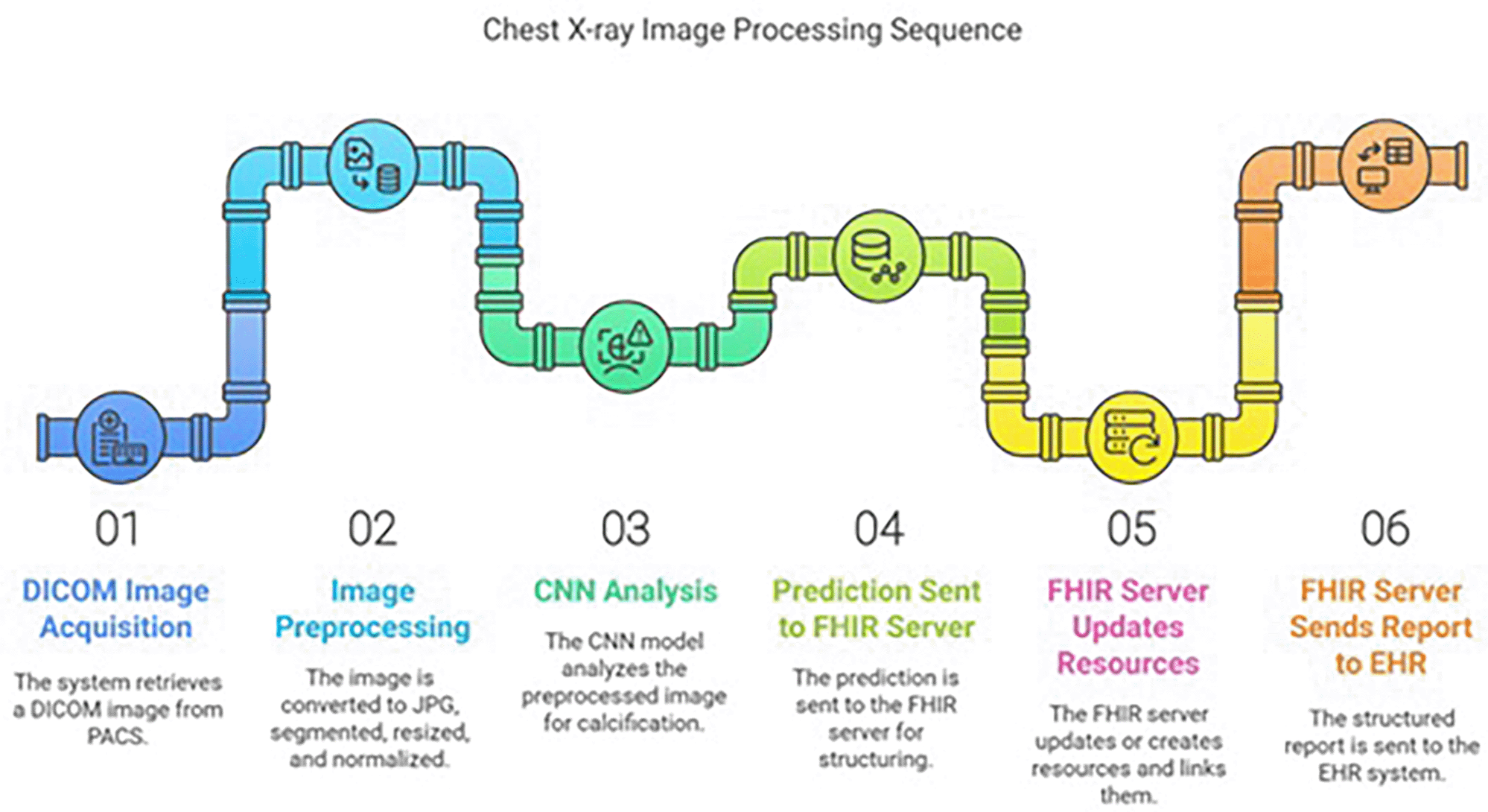
Figure 13. Image processing sequence.
Upon completion of the prediction, a JSON file is generated (as illustrated in
Figure 14). This comprehensive file includes the initial data received from the PACS and the model’s results. Serving as a complete record of the prediction process, this file facilitates traceability and subsequent analysis. Furthermore, this simplified file can be used to generate the final FHIR message.
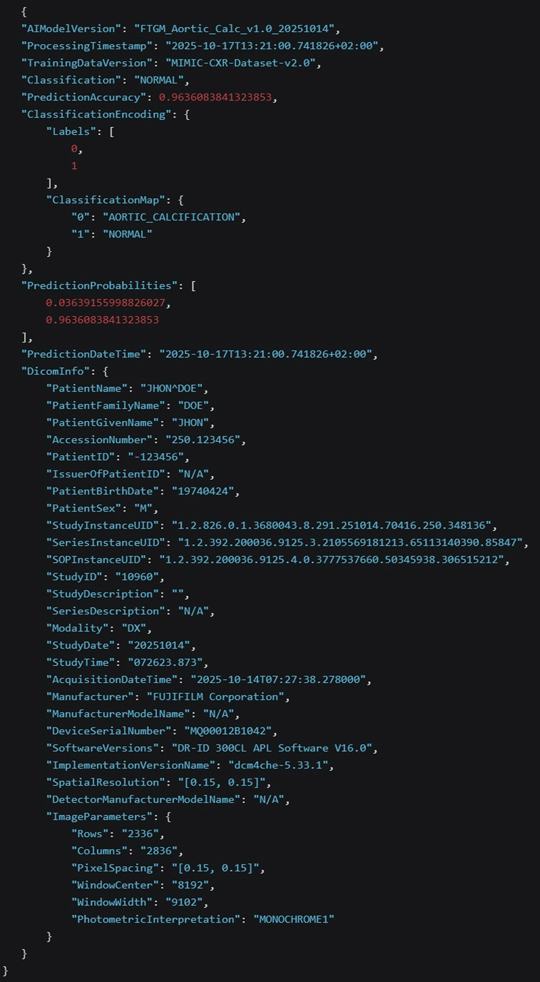
FIgure 14. Structure of the AI prediction JSON intermediary file.
The FHIR output document presented in
Figure 15 is the direct result of a dedicated conversion process applied to an initial source file. This transformation was executed using a bespoke Java implementation, which leverages the powerful capabilities of the widely-adopted Hapi FHIR library.31

Figure 15. Composition of the HL7 FHIR output bundle.
This custom conversion strategy was developed to ensure an accurate and faithful translation of the source data structure and content into a valid, interoperable Fast Healthcare Interoperability Resources (FHIR) format. The choice of the Hapi library, a leading open-source Java API for FHIR, was crucial, as it provides robust tools and a comprehensive set of classes necessary for parsing, validating, and generating complex FHIR resources, thereby guaranteeing adherence to the established international healthcare data standards.
The primary objective of this process is to facilitate the seamless exchange and utilization of the data likely pertaining to clinical information such as aortic calcification recognition within modern healthcare IT ecosystems, where FHIR has become the standard for data communication and interoperability.31
In this implementation the FHIR server used is the Nextgen Mirth connect Enterprise Service Bus (ESB)28 that is capable of interpreting the FHIR specification and is dispatching the information to the EHR system.
Results
The following
Table 7 compares the performance metrics of the proposed model with the other CNN architectures on the training, validation, and test datasets including training time for each model.
Table 7. Performance of CNN models on train, validation, and test sets with training time.
| Model | Epoch |
Train accuracy (%) | Train loss |
Val accuracy (%) | Val loss |
Test accuracy (%) |
Training time (s) |
|---|
| FTGM | 100 | 97.95 | 0.0666 | 97.45 | 0.0851 | 97.71 | 2075 |
| DenseNet201 | 100 | 98.37 | 0.0499 | 96.18 | 0.0833 | 97.96 | 2162 |
| InceptionV3 | 100 | 97.66 | 0.0750 | 96.82 | 0.0557 | 98.47 | 2099 |
| MobileNetV2 | 100 | 96.74 | 0.0889 | 98.09 | 0.0363 | 96.69 | 2102 |
| NASNetLarge | 100 | 96.60 | 0.1066 | 96.82 | 0.1184 | 92.11 | 2268 |
| ResNet152V2 | 100 | 98.37 | 0.0514 | 97.45 | 0.0549 | 98.22 | 2107 |
| ResNet50 | 100 | 95.54 | 0.1446 | 95.54 | 0.1176 | 93.89 | 2084 |
| VGG19 | 100 | 97.17 | 0.0765 | 98.73 | 0.0683 | 96.44 | 2096 |
High-performing models with efficiency focus
FTGM emerges as the most computationally efficient model, achieving a validation accuracy of 97.45% with the shortest training time of 2,075 seconds (approximately 35 minutes). This exceptional efficiency makes FTGM a compelling choice for practical applications where computational resources are limited or training time is a critical constraint. Among the top-performing models, FTGM stands out not only for its competitive accuracy but also for its outstanding speed advantage over more complex architectures.
Comparative Performance Analysis:
While VGG19 achieves the highest validation accuracy at 98.73%, it requires 2,096 seconds of training time, representing a marginal improvement over FTGM’s accuracy at the cost of increased computational demand. Similarly, InceptionV3 (96.82% accuracy) and DenseNet201 (96.18% accuracy) require 2,099 and 2,162 seconds, respectively, demonstrating that increased training time does not necessarily translate to proportional gains in accuracy. This reveals a critical efficiency trade-off in modern deep learning: FTGM achieves near-peak performance with minimal computational overhead.
Specialized Use Cases:
MobileNetV2 offers compelling performance for mobile and edge computing scenarios, achieving 98.09% validation accuracy in 2,102 seconds. However, FTGM still outperforms it in terms of training efficiency, making FTGM the preferred choice for resource-constrained environments.
Conversely, ResNet50 achieved the lowest validation accuracy at 95.54% with a training time of 2,084 seconds, indicating suboptimal performance in both accuracy and efficiency metrics. NASNetLarge, while attempting to leverage neural architecture search principles, required the longest training time (2,268 seconds) without achieving compensatory accuracy gains, making it unsuitable for time-sensitive applications.
Summary of model comparison results:
The FTGM model represents an optimal balance between accuracy and training efficiency, making it the most practical choice for real-world deployments. With a validation accuracy of 97.45% achieved in just 2,075 seconds, FTGM outperforms more complex architectures in terms of the accuracy-to-computation-time ratio. For applications where both high accuracy and computational efficiency are paramount, FTGM is the recommended solution. The choice of alternative models should be driven by specific application requirements: VGG19 for maximum accuracy in high-resource environments, or MobileNetV2 for deployment on edge devices, while FTGM remains the universal optimum for balanced performance.
Figure 16 shows the final accuracy and loss values achieved by the models considered in this study.
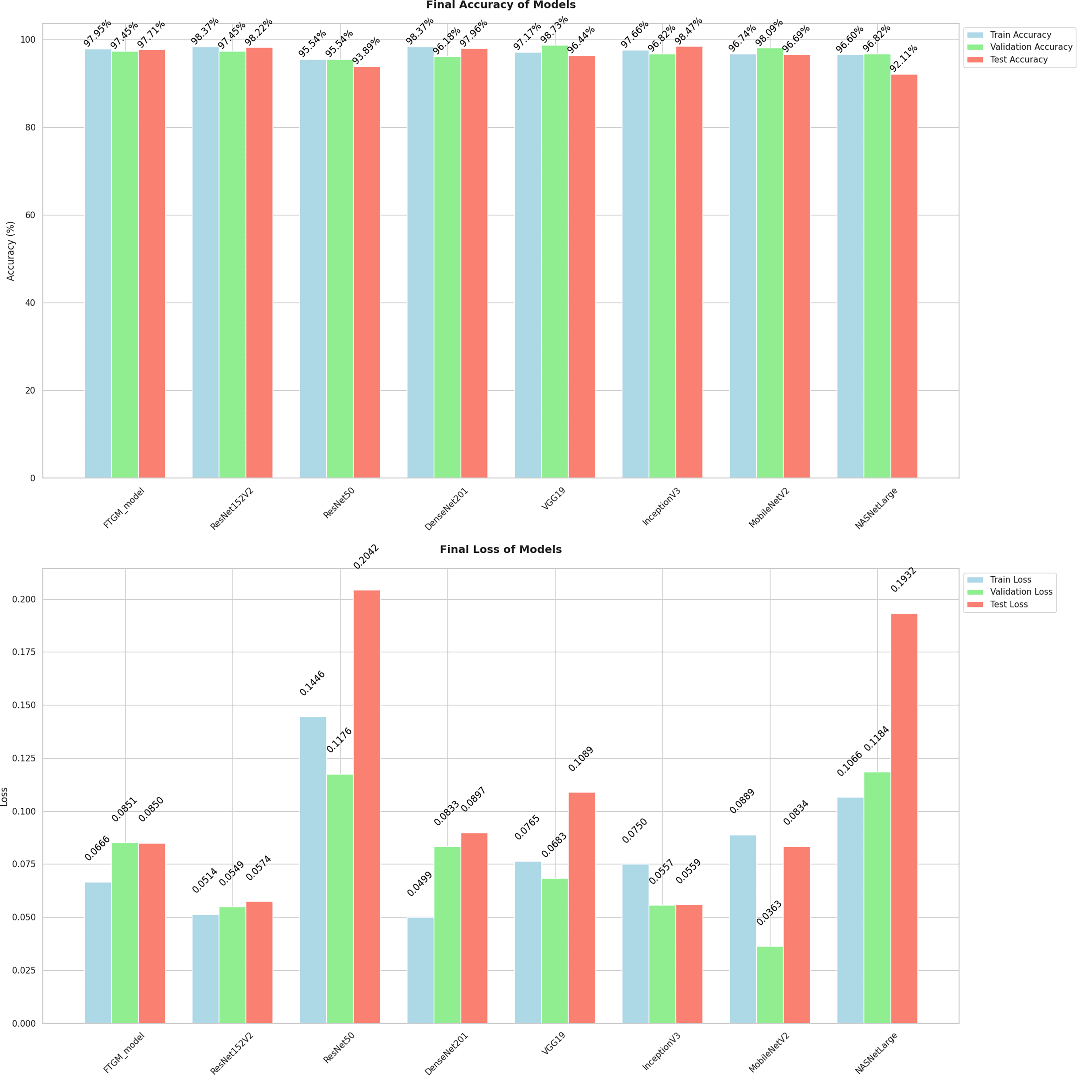
Figure 16. Final accuracy and loss of models.
Figure 17 presents a comparison of the test accuracies achieved by the deep learning models evaluated in this study.
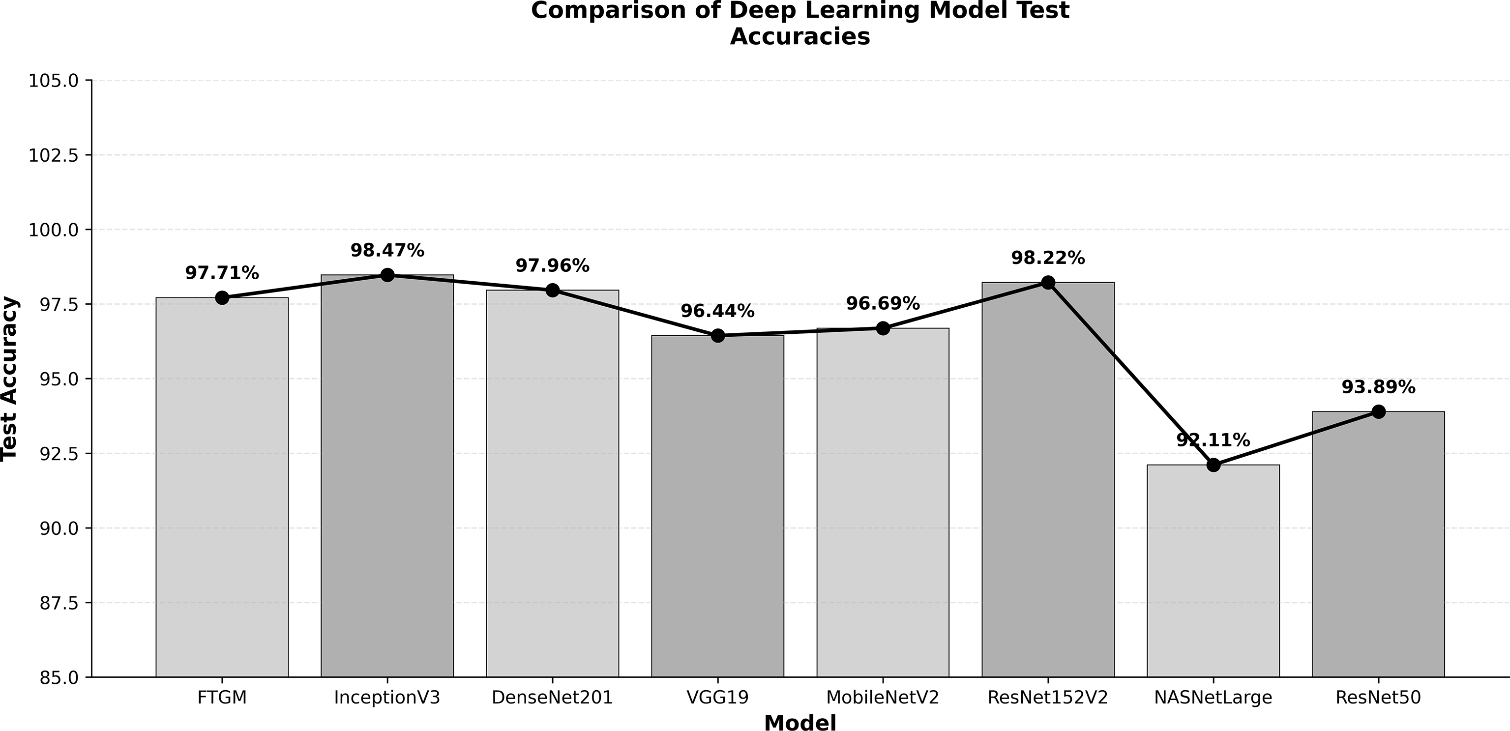
Figure 17. Comparison of deep learning model test accuracies.
Discussion and limits
Our study highlights the feasibility and potential of using deep learning for automated aortic calcification detection in chest radiographs. The high precision and recall achieved by our CNN model, even with a relatively small dataset from a single institution, suggest its robustness in identifying calcification patterns. The choice of a streamlined preprocessing pipeline was crucial in achieving efficient processing. By incorporating steps like lung segmentation, we were able to reduce the computational burden without compromising diagnostic accuracy. This focus on efficiency opens doors for deploying the model on devices with limited processing capabilities, potentially enabling point-of-care diagnostics and expanding access to timely analysis, particularly in resource-constrained settings.
However, our study has limitations. The single-center nature of the dataset may limit the generalizability of the findings to other populations and imaging equipment. Future research should focus on validating the model with external, multicenter datasets to ensure its broader applicability. Furthermore, while our model demonstrates excellent performance in detecting the presence of calcification, quantifying the severity of calcification remains a crucial next step. Future work will explore incorporating quantitative measures, such as the Agatston score,32 into the model’s output to provide a more comprehensive assessment of disease progression. Finally, integrating the model into existing clinical workflows and evaluating its impact on radiologist performance and patient outcomes will be essential for successful translation into clinical practice. Despite these limitations, our findings provide a strong foundation for future research and development in AI-driven cardiovascular imaging, paving the way for improved diagnostic accuracy, efficiency, and ultimately, patient care. The practical implementation of Fast Healthcare Interoperability Resources (FHIR) integration within existing healthcare IT infrastructure, particularly for a project involving clinical data like the recognition of aortic calcification, presents a multitude of complexities. Significant challenges inherently arise in several key areas. Firstly, data mapping requires meticulous attention, as converting legacy or proprietary data models into the standardized, resource-based structure of FHIR demands sophisticated transformation logic and validation to ensure data integrity and fidelity. The implementation of this specific FHIR pipeline is of manifold importance due to the project’s unique and ambitious target. It involves the direct use and conformance with
European standardization models, which serves to ensure broader interoperability and adherence to a cohesive regional framework for health data exchange. Furthermore, it represents a unique and highly practical approach to direct conversion applied to real-world examples. This hands-on application of FHIR standards to complex, live clinical data, is a crucial step, moving beyond theoretical models to demonstrably achieve seamless data flow and standardized interpretation in a live clinical context. This real-world conversion effort validates the FHIR model’s effectiveness in bridging disparate healthcare systems and streamlining clinical research and decision support tools.
Conclusion
This research convincingly demonstrates the substantial potential of deep learning, particularly using a Convolutional Neural Network (CNN) architecture, for the automated detection of aortic calcification directly from standard chest radiographs. Our model, trained on a carefully curated dataset and enhanced by a streamlined preprocessing pipeline, has exhibited high precision and recall in identifying calcification patterns. The efficient processing facilitated by our approach suggests the feasibility of deploying this model on resource-constrained devices, potentially enabling point-of-care diagnostics and broadening access to timely analysis.
The integration of FHIR resources into our workflow ensures seamless interoperability and data exchange with existing healthcare systems, further enhancing the clinical utility of our model. By adhering to FHIR standards, particularly the European Electronic Health Record Exchange Format (EEHRxF), the results generated by our AI model can be readily incorporated into electronic health records (EHRs), facilitating informed clinical decision-making and longitudinal patient monitoring across European healthcare landscapes.
Future research will focus on addressing the limitations of our study, including the single-center nature of the dataset, by validating the model with external, multicenter datasets. Additionally, we aim to expand the model’s capabilities to quantify calcification severity and explore its applicability in detecting other cardiovascular pathologies.
In conclusion, our comprehensive investigation and subsequent development of AI-driven tools for cardiovascular disease management, particularly focusing on aortic calcification recognition via a FHIR-compatible Kinaitics system, mark a significant milestone. This work not only validates the potential of artificial intelligence to augment clinical workflows but also paves the way for a future where these sophisticated tools are seamlessly integrated into everyday clinical practice.
The core impact lies in the profound enhancement of diagnostic accuracy. By leveraging advanced machine learning algorithms trained on extensive datasets, our system can identify subtle yet critical indicators of aortic calcification with a consistency and speed that complements and often exceeds current manual interpretation. This improved accuracy will lead to earlier and more reliable risk stratification for patients.
Furthermore, this integration is poised to significantly improve patient care. The speed and standardization offered by the AI system will reduce diagnostic turnaround times, allowing for quicker initiation of appropriate therapeutic interventions. The FHIR-based Kinaitics architecture ensures interoperability, facilitating secure and efficient data exchange across different healthcare systems. This connectivity is crucial for longitudinal patient management and collaborative research, ultimately contributing to personalized medicine approaches.
The successful implementation and validation of this system represent a fundamental transformation in the landscape of cardiovascular disease management. It moves the field towards a data-driven, proactive model of care, empowering clinicians with powerful, objective decision-support tools. This transformation promises to optimize resource utilization, reduce clinical variability, and elevate the overall quality of care, solidifying the role of AI as an indispensable partner in modern cardiology.
Generative Artificial Intelligence (AI) tools were utilized for the preparation of
Figures 1, 2, and 13 (specifically Napkin, available at https://www.napkin.ai/) and for the correction of English grammar and phrasing within the manuscript (using Gemini 2.5).
Ethics and consent
This study is based on analysis of AP (Antero-Posterior) chest X-ray images obtained from one source: retrospective de-identified chest radiographs, extracted from CT scans, from the Fondazione Toscana Gabriele Monasterio (FTGM) institutional Picture Archiving and Communication System (PACS), executed during common encounters as a routine clinical imaging and retained for clinical documentation of patient care, quality assurance and research purposes.
All DICOM files used in this research were thoroughly anonymized by removing personally identifiable information, including patient names, gender, medical record numbers, date of birth, and date of execution of the exam. Images with potential for identification, like unique clinical signs and symptoms, were also excluded from the dataset. The AI model development and validation were strictly processed in a secure processing environment and did not involve direct human subjects’ contact, intervention, or identifiable health information.
Ethical approval
Ethical approval for this study was granted by the institutional ethics committee of the Comitato Etico Regione Toscana - Area Vasta Nord Ovest (CEAVNO), based at the Azienda Ospedaliero-Universitaria Pisana, Italy (Approval/Permit Number: 26533). This committee is the official affiliated review board for the institution where the research was conducted. No independent review board was used The research was conducted in compliance with the principles of the Declaration of Helsinki and adhered to the ethical guidelines of the European Union and Italian healthcare regulations regarding retrospective data analysis.
Informed consent
It is the standard clinical procedure at the Fondazione Toscana Gabriele Monasterio that all patients undergoing a medical examination, including chest X-rays, provide written informed consent for their procedure. The study exclusively utilized chest X-ray images from adult participants, and no minors were included in the dataset. All DICOM files were de-identified prior to analysis, removing all personally identifiable information. The AI model development and validation were strictly processed in a secure processing environment and did not involve direct human subjects’ contact, intervention, or the use of identifiable health information.







