1. Introduction
1.1 Cetacean bioacoustics and passive acoustic monitoring
Over the past few decades, Passive Acoustic Monitoring (PAM) has become a widely-used, non-invasive tool for tracking acoustically active species over time,1 especially when environmental conditions make visual sightings logistically impossible. As researchers increasingly deploy PAM across multiple sites and extended timeframes, they generate massive datasets that require highly advanced analytical frameworks. Monitoring cetaceans2 is one of the most challenging applications of this technology. Marine mammals produce a variegated repertoire of vocalizations across wide frequency bands, frequently in habitats heavily disrupted by intense human noise. Because of these environmental complexities, maintaining high accuracy in population monitoring is vital for effective marine conservation.
Growing human impacts on marine ecosystems have intensified the need for comprehensive, large-scale conservation efforts. Since marine mammals rely almost entirely on sound to communicate, navigate, and forage, PAM serves as the foundation for studying these vulnerable species. Visual surveys are limited by weather conditions and human bias, whereas PAM allows researchers to track marine life continuously and scale their efforts efficiently across both coastal waters and remote offshore environments.3 On a technical level, underwater microphones called hydrophones capture these vocalizations by converting pressure changes into electrical signals. When paired with low-noise preamplifiers, these systems generally operate at sampling rates up to 200 kHz. The push is to expand PAM networks to map cetacean distributions and behaviors, which is particularly vital for minimizing harmful interactions with commercial fisheries.4
Once the audio is digitized at high frequencies, operators can either monitor the signals in real time for immediate detection or archive the recordings for later study. Both approaches rely on a mix of manual audio-visual inspection and advanced automated workflows.5 Whether analyzed by humans or algorithms, the processing pipeline relies on a shared visual foundation: the spectrogram. Generated via the Short-Time Fourier Transform (STFT), the spectrogram converts raw time-domain signals into a two-dimensional time-frequency image. This visual format is ideal for identifying tonal vocalizations such as whistles, which appear as smooth, continuous, frequency-modulated lines that stand out clearly against sharp, impulsive sounds like echolocation clicks or background static.5 The field has steadily shifted away from manual spectrogram reviews toward automated detection. Early digital signal processing (DSP) techniques—such as template matching,6 active contour methods,7 and entropy-based detectors8—contributed to automated whistle identification. Today, however, deep learning approaches have largely taken over, with convolutional neural networks (CNNs) analyzing spectrogram images directly to deliver far superior detection accuracy.
1.2 Deep learning for cetacean PAM: state of the art
Convolutional neural networks have become the most widely diffused architecture for detecting cetacean vocalizations via spectrograms, improving traditional signal-processing methods across various tasks and species. Jiang et al.9 presented a two-stage pipeline in which an initial CNN detects if a brief spectrogram frame contains a whistle, and a second network classifies the sound by species, distinguishing between killer whales and long-finned pilot whales. This has been obtained utilizing small grayscale spectrogram tiles; they achieved 97% detection and 95% classification accuracy. This success proved that compact, single-channel inputs can effectively capture the geometric shape of whistle contours, provided that the frequency limits and frame durations are carefully selected. While Jiang et al.9 focused on pre-rendered spectrogram images, Shiu et al.10 showed that these models could adapt to varying recording conditions by using a different input format. Instead of treating the spectrogram as a standard visual image, a two-second audio clips is extracted, and then calculated the Short-Time Fourier Transform (STFT) is calculated using a 128 ms Hann window with a 50 ms step size. This process generated a matrix of time-frequency magnitude values, which they normalized using the squared Frobenius norm and passed directly into the CNN as a numerical tensor. When tested on North Atlantic right whale upcalls between 39 Hz and 358 Hz, their model delivered significantly better precision-recall metrics and cut false positives per hour by orders of magnitude compared to existing baselines. The model maintained its high performance on entirely new recordings from different times and locations, successfully passing the real-world stress test that operational passive acoustic monitoring systems regularly encounter.
Li et al.11 utilized a depthwise-separable CNN to classify multiple types of whistles from Indo-Pacific bottlenose dolphins (Tursiops aduncus). They used three-channel spectrogram inputs combined with a comprehensive set of time-domain data augmentations, including pitch-shifting, time-stretching, noise mixing, temporal shifting, and gain adjustments. Classification accuracy increased from 93.7% on the original samples to 98.53%, proving that data augmentation can effectively offset the challenges of small training sets and unbalanced classes. In this study, the authors admitted that their chosen STFT parameters might not represent the ideal spectrogram configuration for whistle classification, treating the spectrogram generation as an arbitrary choice rather than an optimized variable.11
Passing from simple binary detection to tracing the exact paths of vocalizations, researchers like Jin et al.12 have reframed the challenge as a semantic segmentation task. Their model processed high-resolution grayscale spectrograms to generate pixel-level masks of whistles, which were then refined using morphological post-processing to map out centerlines and untangle overlapping calls. Despite evaluating their model on noisy coastal recordings filled with snapping shrimp interference, they achieved a precision of 0.96, an accuracy of 0.89, and an F-score of 0.86. These results show that dense, high-resolution inputs are essential when a study needs to preserve precise contour curves and thickness for subsequent bioacoustic analyses. Taking a different approach, Nur Korkmaz et al.13 investigated the potential of transfer learning for dolphin whistle detection. Single-channel grayscale spectrograms have been duplicated into a three-channel format, and a pre-trained VGG16 network using automated hyperparameter optimization. This method achieved a 92.3% mean accuracy on a substantial, annotated dataset, easily outperforming traditional detectors while keeping the initial preprocessing straightforward. Their work underscores the practical benefit of adapting established computer-vision models when annotated underwater audio datasets are scarce. Based on these studies, the way input data is represented is just as critical to performance as the neural network design itself. Small, single-channel tiles work well for basic detection and generalize efficiently with minimal computing power, three-channel inputs allow researchers to leverage powerful pre-trained models, and high-resolution imagery preserves fine pixel-level details of sound contours. Ultimately, these findings reveal that preprocessing steps like frequency filtering, STFT configuration, and image scaling are not minor technical details but major factors driving model success. While this reality is widely accepted in theory, the field still lacks a rigorous, quantitative evaluation of how these preprocessing choices interact within a unified, reproducible pipeline for cetacean monitoring.14
A second, related challenge concerns the annotation of training data. The studies reviewed above employ diverse and largely undocumented labeling conventions: event boundaries, minimum duration thresholds, and the criteria for distinguishing whistle from click train or burst pulse are rarely made explicit. This fragmentation has been identified as a systemic limitation of bioacoustic machine learning more broadly, and is compounded at the species level by terminological inconsistency in the T. truncatus vocalization literature, where identical acoustic events have historically received different labels across research groups.15 Inter-annotator variability in marine PAM contexts has been shown to depend on both vocalization type and signal-to-noise ratio,16 introducing a source of performance variance that is rarely quantified in comparative studies. The proposed pipeline addresses this gap by formalizing an annotation protocol with explicit decision criteria for each label class (Section 2.2). The present work consolidates these insights into a unified, formally defined framework that makes preprocessing decisions explicit, reproducible, and systematically configurable.
1.3 Objectives and contributions
Objective 1 — A formally described, six-stage methodological framework. The proposed pipeline formalizes each stage of the CNN-based detection workflow — from annotation protocols and segmentation strategies through spectrogram parameterization and preprocessing to cross-validation design and performance reporting — making every decision point explicit and reproducible. Each stage generalizes to other taxa and vocalization types through YAML-based configuration.
Objective 2 — A full open-source implementation: ai-pam-pipeline. The toolkit provides a command-line interface whose entire parameter space is defined by a single YAML experiment file, ensuring that any reported result can be exactly regenerated. A plug-in architecture allows the CNN model to be substituted without modifying the training loop. Full technical documentation is provided as Extended Data.
Objective 3 — End-to-end validation on two complementary tasks. The framework is demonstrated on (A) a binary whistle detector for T. truncatus with cross-domain evaluation on an independent open-ocean dataset, and (B) a five-class vocalization classifier on the same training set, exercising the multiclass configuration and the scroll augmentation mechanism. Together, the two experiments show all six pipeline stages operating as an integrated, reproducible workflow.
2. Materials and methods
2.1 Overview and design principles
Implementing deep learning in Passive Acoustic Monitoring (PAM) requires a coordinated sequence of interdependent steps. The process begins with raw data analysis, in which PAM operators screen recordings to extract, identify, and classify individual signals. These signals are then converted into spectrogram images, a step that involves choosing among a wide range of parameters — color scales, image resolution, and STFT settings — each of which can meaningfully affect the outcome. The resulting images may further undergo preprocessing or augmentation to compensate for data scarcity, followed by visual inspection to verify their quality. This stage alone can be time-consuming and prone to undetected inconsistencies in training data composition. Once the image dataset is assembled, model training can proceed.
In practice, the full pipeline is rarely described in its entirety, let alone standardized. Yet undocumented workflows directly undermine reproducibility: CNNs are inherently stochastic and sensitive to parameter choices, so even minor untracked variations can produce divergent outcomes. The framework proposed here addresses this by formalising the entire workflow into six integrated stages (
Figure 1), all governed by a single configuration file. The sequence spans from raw data annotation (Stage 1) to final performance evaluation (Stage 6), with intermediate steps covering audio segmentation into discrete windows (Stage 2), spectrogram generation (Stage 3), optional image filtering for feature enhancement (Stage 4), and CNN model training (Stage 5).
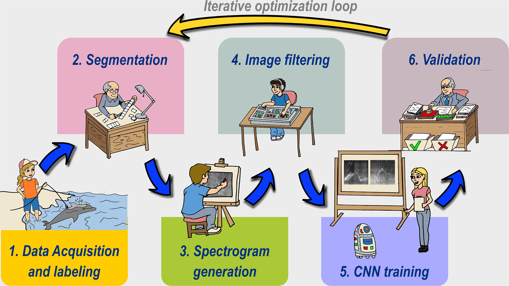
Figure 1. Six-stage pipeline block diagram of ai-pam-pipeline.
Module names are annotated for each stage. Architecture-level labels use general PAM terminology; inline annotations report the cetacean validation parameters adopted in Section 3 as an example instantiation.
2.2 Stage 1 — Audio acquisition and PAM annotation (
Figure 1)
In PAM applications, data acquisition at monitoring sites is typically carried out using autonomous devices equipped with a hydrophone, which converts acoustic waves into an electrical signal, followed by a preamplifier, an analog-to-digital converter (ADC), and a recording system. Depending on the target species and the type of vocalization of interest (e.g., tonal or pulsed signals), the relevant signal bandwidth may range from a few hertz up to approximately 25 kHz, as is typical for bottlenose dolphin whistles, and extend beyond 160 kHz for high-frequency echolocation clicks. Consequently, the sampling rate must be selected accordingly, in compliance with the Nyquist criterion, typically adopting values of 96, 192, or 384 kS/s. The acquired data are usually stored on integrated memory media, in WAV format or in lossless compressed formats such as FLAC. In long-term monitoring deployments, recordings are typically partitioned into fixed-duration segments (e.g., 1, 5, 30, or 60 minutes). It is considered best practice to adopt a standardized naming convention that includes a timestamp in a convenient format, such as YYYYMMDD_hhmmss. When multiple recording units are deployed, prepending a unique station ID (e.g., HYD1_) and appending the sampling rate (e.g., _192) is highly recommended to ensure traceability. Such structured filenames are fundamental for enabling downstream automated processing and metadata extraction. The acquired data subsequently undergo extensive processing aimed at detecting vocalizations, which may be performed through visual and acoustic inspection by trained personnel and/or with the support of detection software such as PAMGuard. This annotation process, in which segments of recordings are labeled by associating specific tags with particular vocalizations, remains — as previously highlighted — non-standardized.16 In the case of Tursiops truncatus, there is not even a universally accepted classification of the different vocalization types. The proposed approach consists of leveraging the tagging functionalities available in the open-source software Audacity (or similar tools). The user can graphically select portions of the audio signal containing specific sounds and assign them a label. Labels may overlap in the case of superimposed sounds. The final output is a tab-separated values (TSV) file containing three main fields:
,
, and
. The first two represent the temporal offsets, expressed in seconds as floating-point values, relative to the beginning of the recording. Audacity supports a variety of audio formats (e.g., WAV, FLAC), while labels are exported as plain text (TXT) files. To facilitate automated pairing within the pipeline, it is strongly recommended that label files maintain the same stem as the source audio file (e.g., HYD1_20200101_100025_192.txt). In this work, a simplified tagging scheme was adopted for the general detection of whistles produced by Tursiops truncatus:
W (whistle): tonal, continuous, frequency-modulated signal with a smooth contour in the spectrogram.
MW (multiple whistle): segments containing overlapping whistles.
ECT (click train): regular series of broadband pulses, typically appearing as vertical striations.
BPS (burst pulse sound): rapid bursts of irregular pulses.
FB (feeding buzzes): dense vertical texture associated with foraging activity.
NOISE: vessel interference, flow noise, and non-target biological sounds.
The same approach can be extended by adopting a more articulated labeling scheme or by applying the same principles to other species. Although a standardized classification framework would be desirable, in its absence, it is essential to maintain a consistent labeling criterion across all stages of the processing pipeline. The establishment of a universally shared annotation scheme would significantly increase methodological consistency and facilitate inter-calibration across diverse research efforts. For example, a classification approach similar to the FAO alpha-3 codes, employed for fish species classification, could be adopted.
An advantage of maintaining paired audio and label files is the ability to extract specific tagged and classified fragments automatically, ensuring consistency and replicability across large datasets. It could also facilitate the systematic creation of specialized databases, where vocalizations are indexed by type and optionally integrated with metadata (date, time, and environmental parameters).
2.3 Stage 2 — Audio handling, segmentation and windowing
Inference models based on neural networks require input data with strictly defined dimensions. Whether the architecture operates directly on the raw acoustic signal or on spectrogram representations, a fixed temporal observation window must be established. A wider window can capture finer acoustic details and potentially improve detection resolution, though this comes at the cost of reduced system responsiveness in real-time applications and greater computational overhead at inference time. Narrower windows, conversely, allow faster response and lower resource consumption, but may fail to capture the contour features that define a vocalization, with a corresponding effect on model metrics. In the work of Scaradozzi et al., which used the pipeline described here for the detection of T. truncatus whistles, a 0.8-second frame proved effective for capturing the bioacoustic modulation of interest.17 For continuous temporal analysis, overlapping consecutive windows is standard practice, preventing signals from being split across boundaries and subsequently misclassified. That study employed a 50% overlap, generating a new observation window every 0.4 seconds. These values are adopted throughout the present work as the cetacean validation parameters; other taxa or vocalization types may require different window lengths, all of which are configurable in the YAML experiment file (e.g., pipeline.stage_2.as_len, pipeline.stage_2.as_overlap). Species with longer stereotyped vocalizations — such as the song units of mysticetes or the multi-second call sequences of some odontocetes — are accommodated by increasing as_len accordingly, with no further modification to the pipeline. The choice of window size and overlap also has direct implications for real-time deployments, particularly on edge devices with constrained computational resources.18 When a tagged signal is shorter than the defined window, ai-pam-pipeline automatically centers the acoustic event within the frame to preserve spatial consistency for the CNN.
Isolating signals by class and rigorously excluding target-class events from the background class are essential to prevent inconsistency during training. Without this, the CNN risks learning to distinguish not between pure background and the target bioacoustic feature, but between categories that are acoustically contaminated by one another. The problem is especially acute in multi-class settings, where training samples labeled for one vocalization type must not contain fragments of another: such contamination introduces ambiguity directly into the feature space. To address this, the library implements an automated padding mechanism that expands exclusion zones around each annotation boundary as a function of the sliding window step; the technical details of this logic are provided in the Extended Data.
In PAM recordings where multiple vocalization types co-occur simultaneously, this exclusion and erosion logic becomes the primary means of obtaining acoustically unambiguous training samples. The mechanism is fully general: any annotation class whose temporal extent overlaps with the target class generates an exclusion zone, and the morphologically eroded residual of the target span defines the sampling domain for that class. The design applies identically regardless of species or vocalization type, provided the annotations follow the label-file convention described in Section 2.2.
Figure 2 illustrates this process for an exemplary extraction from a multi-label recording. The target species is Tursiops truncatus and the class of interest is the echolocation click train (ECT), but the same logic applies to any acoustic class in any annotated PAM dataset. Panel A shows the raw Audacity label file, in which NOISE, BPS, W, and ECT annotations are present and temporally overlapping. Panel B traces the construction of the final usable ECT signal: the raw ECT span (C3_raw) is first reduced by the exclusion zones generated from the overlapping NOISE, BPS, and W annotations (C3_post_excl), after which a one-dimensional binary erosion (C3_eroded) is applied using a structuring element of length equal to the minimum duration expressed in frames. The operation acts on the binary timeline representation, where active frames denote the presence of the target class after exclusion filtering. The effect is inherently contractive: by shrinking each contiguous active segment at both boundaries, it eliminates residual fragments that contain insufficient signal. Panel C shows representative spectrogram tiles extracted from the eroded span, each containing an unambiguous click train free of contamination from adjacent vocalizations. The exclusion zone width is parametrically controlled by the analysis window length and step size, as detailed in the Extended Data.
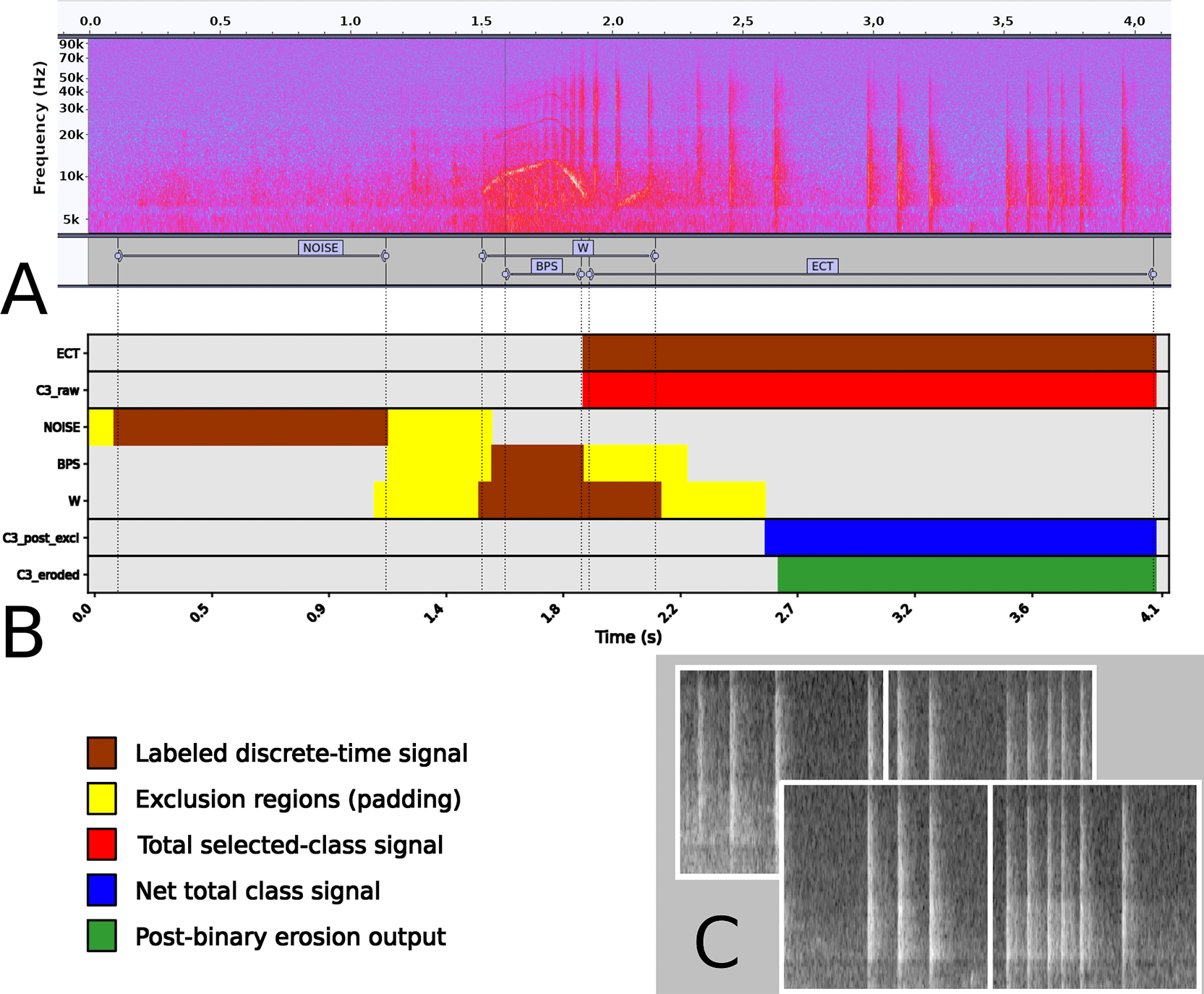
Figure 2. Multi-step segmentation and exclusion logic for class-specific sample extraction from a dense multi-label acoustic recording.
(A) Raw Audacity label file: four annotation classes (NOISE, BPS, W, ECT) are present and temporally overlapping in a
s segment. (B) Construction of the usable ECT (C3) signal: the raw ECT span (C3_raw) is reduced by exclusion zones derived from all overlapping non-target annotations (yellow), yielding the net usable signal (C3_post_excl, blue) and its morphologically eroded version (C3_eroded, green), which constitutes the final sampling domain for spectrogram window extraction. (C) Representative
spectrogram tiles extracted from the eroded span, showing uncontaminated echolocation click trains. Although the example is drawn from a T. truncatus recording, the exclusion and erosion procedure is identical for any class in any annotated PAM dataset.
An additional mechanism for expanding the training set is scroll augmentation: for a given annotated event, the analysis window is slid from the position where only the minimum required vocalization duration appears at the right edge, generating multiple time-shifted copies of the same event. This is the primary data augmentation strategy implemented in ai-pam-pipeline, activated via the YAML parameter pipeline.stage_2.augmentation_scroll. Image processing filters (Section 2.5) can also serve as a basis for augmentation: applying one or more transformations to a clean spectrogram — for instance, adding synthetic pink noise at varying intensity levels to a whistle image — produces training samples spanning a range of apparent signal-to-noise ratios. This approach is fully supported within the framework: running Stages 2–4 with different filter configurations and merging the resulting spectrogram directories before training is sufficient to compose a multi-condition dataset without any modification to the pipeline.
2.4 Stage 3 — Spectrogram generation
As summarized in
Table 1, the most widely adopted methodological approach involves the use of Convolutional Neural Networks (CNNs) that process spectrograms as input. Spectrogram images are generated via the discrete STFT, defined as:
where
represents the window function,
is the discrete time index, and
is the hop size. In this framework, a Hanning window is applied to minimize spectral leakage. The hop size
is dynamically calculated based on the chosen FFT length (
) and the overlap percentage (
), following the relation
Table 1. Summary of CNN-based cetacean whistle detection studies reviewed in Section 1.2.
| Study | Species/call type | Input repr. | Size | Ch. |
Task | Preprocessing treatment |
|---|
| Jiang9 | Killer/pilot whale | Grayscale image | ~180 × 120 | 1 | Det. + Class. | Fixed band-limiting & frame duration. |
| Shiu10 | N. Atl. right whale | Num. matrix | 40 × 40 | 1 | Binary Det. | Fixed STFT (128 ms Hann, 50 ms adv.) |
| Li11 | T. aduncus | RGB image | 200 × 200 | 3 | Multiclass | Fixed STFT; acknowledged as non-optimal. |
| Jin12 | T. truncatus | Grayscale image | 1000 × 1000 | 1 | Sem. Segm. | Fixed high-res for contour fidelity. |
| Korkmaz13 | Dolphin whistle | RGB image | 224 × 224 | 3 | Binary Det. | Minimal and fixed for VGG16. |
To align the representation with the logarithmic perception of sound intensity and to compress the dynamic range for the CNN, the magnitude of the STFT is converted to a decibel (dB) scale:
The spectrogram image generation process must allow for the systematic and uniform adjustment of core acoustic parameters, such as the FFT size (
) and the Hanning window overlap. Additionally, it must support customizable visualization settings, including output image dimensions (width and height) and the selection between grayscale representations or specific predefined colormaps. In the experiments reported in Section 3, the grayscale mode is used throughout with an image size of
pixels. This differs from the
format adopted in the reference architecture,17 reflecting an updated preprocessing choice evaluated as part of the present framework.
While band-pass filtering in the time domain is a common practice, the proposed library performs frequency selection directly on the generated spectrogram. This spectrogram cropping restricts the analysis to a specific frequency range
, effectively discarding components outside the bandwidth of interest. In the case of T. truncatus whistle detection, a frequency crop in the range of 3–25 kHz is generally employed, as determined by the species’ whistle bandwidth. This range encompasses the most discriminative frequency-modulated contours of the species while optimizing the input dimensionality for the CNN. The image dimensions (width_px, height_px) are likewise decoupled from the window length: a longer analysis window produces a wider raw spectrogram that is resampled to the same fixed pixel grid, preserving CNN input consistency regardless of species. By restricting the vertical axis of the spectrogram image to these limits, the pipeline ensures that the model focuses on the biologically relevant signal features, improving both classification accuracy and computational efficiency during inference. The heterogeneity of spectrogram formats across the literature (
Table 1) underscores the value of recording every STFT setting explicitly in the configuration file, so that the representation used in any given study can be reproduced without ambiguity. The adoption of a single-channel grayscale representation provides distinct computational advantages, particularly for deployment in resource-constrained environments. By reducing the input dimensionality from the three channels required by standard RGB images to a single data stream, the model minimizes memory footprint and processing overhead.
2.5 Stage 4 — Spectrogram image preprocessing
While raw spectrograms provide a fundamental time-frequency representation, they often suffer from non-uniform background noise, low contrast, and interference from anthropogenic sources. Preprocessing the spectrogram can substantially improve the signal-to-noise ratio of target vocalizations — particularly the frequency-modulated contours of dolphin whistles — making it easier for the model to extract the relevant features and learn to recognize them reliably.19 This step is optional in the proposed pipeline, but if it is used, it must be applied with strict consistency: the same transformations that are applied to the training data must be applied identically to every input processed by the inferential model during detection and classification.17 In real-time deployments, the computational cost of these filters also deserves careful consideration, as it directly affects system responsiveness. In PAM applications, filtering is commonly applied to the raw acoustic signal21 to attenuate background noise or bring out vocalization features that would otherwise be difficult to detect. Conversely, applying filters to the spectrogram image does not involve the original signal, but rather operates directly on the time-frequency representation generated via STFT before it is fed into the neural network. While this image-based approach is widely established in computer vision — for instance, in the enhancement of underwater photography22 — it remains relatively unexplored within the context of cetacean vocalization detection.
The toolkit supports a set of standard image-domain filters from OpenCV — including morphological operators (Top-Hat), edge detectors (Laplacian, Canny, Sobel, Scharr), and adaptive contrast enhancement (CLAHE) — that can be applied individually or in combination to the raw spectrogram before CNN input. A global polarity inversion is also available. The complete filter specifications are documented in the Extended Data.
Beyond image filtering, Stage 4 includes a normalization step applicable to each spectrogram image prior to CNN input. Per-image normalization rescales the pixel intensity values to the range
independently for each sample, compensating for global amplitude variability across recording sessions, hydrophone sensitivities, and environmental conditions. This operation ensures that the CNN receives input distributions of consistent dynamic range, regardless of the absolute signal level in the original recording, and is a prerequisite for stable gradient-based optimization. In all experiments reported in Section 3, per-image normalization is enabled via the YAML parameter pipeline.stage_4.image_normalization: true and constitutes the only active Stage 4 operation; image-domain filters are not applied in this work.
The toolkit introduced in this study provides a dedicated script, ai_pam_preprocessing.py, designed to execute the operations detailed in Stages 2 through 4 as a unified, streamlined workflow. This script directly interfaces with raw audio recordings and their associated label files to generate spectrograms, optionally filtered, according to the specific experimental parameters encoded in the configuration file described in the following section.
2.6 Stage 5 — CNN training with k-fold cross-validation
As established in Section 1.2, CNNs operating on spectrogram images represent the current standard for automated vocalization detection in PAM. The proposed framework is implemented for CNNs but is not restricted to them: the plug-in architecture convention — any Python file exposing a build_model(input_shape, n_classes, kernel_size) function — allows recurrent (RNN, LSTM), hybrid (CRNN), or transformer-based (ViT) architectures to be substituted without modifying the training loop. For models requiring sequential inputs, the toolkit produces time-series spectrogram extracts by modulating the frame overlap, as described in Section 2.3.
The present study utilizes a baseline CNN architecture,17 specifically engineered for efficiency and deployment on resource-constrained hardware,18 implemented using the TensorFlow framework.20 The network consists of three convolutional blocks with an increasing number of filters (32, 64, and 128, respectively); each block incorporates a Rectified Linear Unit (ReLU) activation and a
max-pooling layer. The architecture concludes with a fully connected layer of 128 neurons and a sigmoid activation function for the binary output layer. For multiclass tasks, the sigmoid output is replaced by a softmax activation over N classes, and the loss function switches from binary to categorical cross-entropy; the model file is passed via the YAML key pipeline.stage_5.model.architecture without other changes to the loop.
The model takes as input single-channel spectrogram images, with 224x224 pixel dimensions consistent with the spectrogram generation parameters described in Section 2.4. Training uses the Adam optimizer with an initial learning rate of 0.0001. The loss function is binary cross-entropy for the binary classification task and categorical cross-entropy in the multiclass setting, reflecting the sigmoid and softmax output activations respectively.
The training process uses a batch size of 32 and a maximum of 100 epochs. A linear learning-rate warmup is optionally applied during the initial epochs to improve optimization stability. Model performance is evaluated using accuracy during training and complemented by additional metrics (e.g., macro F1-score) computed on the held-out data. The training process incorporates an early stopping mechanism with a patience of 10 epochs and a 5-epoch warmup period— designed to prevent premature termination during initial loss plateaus—while ensuring the restoration of the best-performing weights at the end of the session.
To ensure reproducibility, all random processes are controlled via fixed seeds, and model initialization is re-seeded at each fold.
To conclude the model preparation phase, the proposed toolkit provides a dedicated script, ai_pam_train.py, which automates the management of k-fold cross-validation, individual model training, and in-domain validation, ultimately generating the performance metrics discussed in Section 2.7 and managing the training directives (epochs, early stopping, batch size, etc.).
2.7 Stage 6 — Model evaluation and performance measurement
2.7.1 In-domain cross-validation
Once the spectrogram image dataset has been assembled, the framework evaluates model performance through stratified k-fold cross-validation. The full dataset is partitioned into
non-overlapping subsets (folds) of approximately equal size. In each of the
iterations, one fold serves as the held-out test set while the remaining
folds are used for training, including an in-training validation split that governs early stopping. This procedure is repeated until every fold has served once as the test set, yielding
independent performance estimates. In the present study,
and partitioning is performed by random assignment with a fixed seed (seed
), ensuring full reproducibility. For binary classification, the predicted class is determined by applying a fixed threshold
to the sigmoid output: a sample is assigned to the positive class (vocalization present) if the network output exceeds
, and to the negative class otherwise. In the present study the decision threshold is fixed at θ = 0.5, the balanced operating point of the sigmoid output.
2.7.2 Binary classification metrics
Performance is summarized by five complementary metrics computed per fold and then averaged across folds:
• Accuracy
• Precision
• Recall
• F1-score
• False Discovery Rate
Recall and F1-score are the primary metrics of interest in PAM detection tasks, where false negatives (missed target events) typically carry a higher operational cost than false positives. In the cetacean whistle detection context of this study, missed whistles are the more consequential error. Precision is reported separately to confirm that high recall is not achieved at the expense of excessive false alarms.
2.7.3 Multiclass evaluation metrics
For classification tasks involving
classes, the sigmoid output layer is replaced by a softmax activation, and a sample is assigned to the class with the highest predicted probability. Performance is assessed through per-class and aggregate metrics.
Per-class Precision, Recall, and F1. Each metric is computed independently for each class
:
where
,
, and
are the true positives, false positives, and false negatives for class
, respectively. Per-class recall is particularly diagnostic: in the presence of class imbalance, a model may achieve high overall accuracy while suppressing minority classes entirely (
), a failure mode that is invisible to aggregate metrics alone.
Macro-averaged F1. The unweighted mean F1 across all
classes:
Macro F1 is sensitive to minority-class performance and constitutes the primary aggregate metric when all classes are of equal operational importance, regardless of their support in the training set.
Weighted-averaged F1. The support-weighted mean:
where
is the number of true instances of class
. Weighted F1 reflects aggregate performance on the training distribution and may be misleadingly high when the dominant class performs well while minority classes are suppressed; it is reported for reference alongside Macro F1.
Confusion matrix. The full
matrix
, where
is the number of instances of true class
predicted as class
. Normalized by true class (row-normalized), the confusion matrix identifies systematic confusions between acoustically similar classes and distinguishes genuine misclassification from class suppression due to imbalance.
The practical effect of unbalanced training data and annotation incompleteness on these metrics is illustrated in Section 3.4, where a known-imbalanced multiclass configuration on the Oltremare dataset produces the metric patterns described above.
2.7.4 Cross-validation design for multiclass tasks
For multiclass tasks with unequal class frequencies, stratified k-fold cross-validation is recommended to ensure each fold contains a representative distribution of all classes. For the binary balanced design in Experiment A (Section 3.2), standard and stratified k-fold are equivalent. The stratified design is adopted in Experiment B (Section 3.4).
2.7.5 Cross-dataset generalization
In-domain cross-validation provides an estimate of performance on held-out data drawn from the same recording session and acoustic environment as the training set. This upper bound is an optimistic predictor of deployment performance, since real-world PAM scenarios routinely involve equipment, sites, and species that differ from the training conditions. The framework therefore separates in-domain validation from cross-dataset testing as two distinct evaluation stages. Cross-dataset testing is carried out using ai_pam_crosstest.py, which loads a set of trained fold models and evaluates them on an entirely independent spectrogram dataset.
The evaluation was conducted using the all mode: performance metrics are computed independently for each of the
fold models, providing a granular distribution of results.
2.8 Iterative use of the framework
Although the framework is organized into six formal stages, its execution is intentionally iterative rather than strictly linear. When validation performance is unsatisfactory, the experiment can be reconfigured by modifying the YAML file and re-running the pipeline from Stage 2 onward, or, when needed, from any later stage downstream of the unchanged source recordings. In practice, this allows segmentation parameters, spectrogram settings, preprocessing filters, sampling policies, or training hyperparameters to be adjusted without revisiting the original recordings or repeating the manual labeling process. Since annotation is one of the most demanding and time-consuming steps in PAM workflows, preserving the labeled source material while enabling controlled reprocessing is a major operational advantage.
3 Use cases
3.1 Datasets
3.1.1 Oltremare dataset (in-domain)
Acoustic recordings were collected at the Oltremare marine park (Riccione, Italy) in November 2021, as described in Screpanti et al.23 Seven free-swimming Tursiops truncatus were recorded using a UREC U384K autonomous recorder (Dodotronic/Nauta) equipped with a SQ26–05 hydrophone at a sampling rate of 192 kHz. Annotation was performed by a trained PAM operator following the labeling protocol described in Section 2.2, yielding 3,451 whistle segments (label W), 233 multiple whistle segments (label MW) and 2,545 non-whistle segments (labels NOISE, ECT, BPS, FB). Each annotated segment yields multiple spectrogram windows depending on its duration and the configured overlap. Since the primary focus of the labeling performed on the dataset was the detection of whistles, the other vocalizations (ECT, BPS, FB, and NOISE) were only labeled to a limited extent. In particular, a very small number of feeding buzzes were labeled (only 308 segments). The complete annotated dataset is publicly available.24
3.1.2 DCLDE 2022 cross-test dataset
For cross-domain evaluation of experiment A, the DCLDE Oahu dataset was used, which concerns acoustic data collected through a multi-channel towed array hydrophone during the Hawaiian Islands Cetacean and Ecosystem Assessment Survey (HICEAS) in 2017.25 A single recording containing vocalizations of T. truncatus (Acoustic detection number 46) was identified in the dataset, dated July 15, 2017, from 11:09 PM to 11:24 PM (UTC). A specific track (n. 3) was extracted for testing purposes and annotated independently following the same protocol as the Oltremare dataset, yielding 458 whistle segments. This process resulted in 715 whistle spectrograms (positive class) and 1,054 non-whistle spectrograms (negative class). From this pool, 500 spectrograms were randomly sampled for each class— utilizing a fixed seed of 42—to establish a balanced test set for the cross-domain performance evaluation. No DCLDE material was used during training; the dataset is used exclusively for cross-domain evaluation.
3.2 Validation
Two experiments validate the framework on the Oltremare dataset. Both share the same baseline CNN architecture and training protocol; they differ in the number of classes, the spectrogram frequency range, and the augmentation strategy, all of which are controlled through the YAML configuration file without modifying any code.
Experiment A demonstrates the binary whistle detector through all six pipeline stages, including cross-domain evaluation. The positive class (C1) groups whistle and multiple-whistle annotations (W, MW); the negative class (C0) groups all co-occurring non-whistle vocalizations — background noise, feeding buzzes, burst-pulse sounds, and echolocation click trains (NOISE, FB, BPS, ECT). Defining C0 from the full range of non-target vocalizations, rather than from background noise alone, trains the detector to reject the acoustic events that co-occur with whistles in real recordings, which reduces the false-positive rate under operational conditions. Audio was segmented into 0.8 s windows with 50% overlap (Stage 2). Each window was rendered as a 224 × 224 grayscale spectrogram over 3–25 kHz with a 512-sample FFT and 50% STFT overlap (Stage 3), followed by per-image intensity normalization (Stage 4); no image-domain filters were applied. The model was trained under ten-fold stratified cross-validation, balanced at 4,700 samples per class with seed 42 (Stage 5). Stage 6 evaluated each of the ten fold models independently on the DCLDE 2022 cross-domain test set.
Experiment B demonstrates the multiclass configuration of the same framework. Five mutually exclusive classes were defined from the Oltremare annotations: C0 (NOISE), C1 (W/MW), C2 (BPS), C3 (ECT), and C4 (FB). The frequency crop was widened to 3–96 kHz to capture the broadband structure of impulsive vocalizations. Because the feeding-buzz class (C4) had substantially fewer annotations than the others (~600 segments, from 308 single annotations), scroll augmentation was enabled for C4 alone, translating the analysis window in 0.1 s steps to generate multiple time-shifted copies of each event (augmentation_scroll: true, scroll_step: 0.1). The resulting dataset totaled C0: 8,154; C1: 5,834; C2: 1,792; C3: 2,406; C4: 3,694 windows. Training used 2,000 randomly sampled images per class (C2: 1,792, limited by annotation density) under ten-fold stratified cross-validation. Stage 6 was not extended to an external dataset; performance is reported for in-domain held-out data only, as the purpose of Experiment B is to demonstrate framework scalability rather than to characterize cross-domain behavior.
Table 2 lists the YAML key parameters for experiment A.
Table 2. Reproducibility reference for Experiment A: YAML parameter paths and values used in all training runs.
| YAML path | Value (Exp. A) | Description |
|---|
| pipeline.stage_2.as_len | 0.8 | Analysis window length (s) |
| pipeline.stage_2.as_overlap | 0.5 | Window overlap fraction |
| pipeline.stage_3.fft_len | 512 | FFT window size |
| pipeline.stage_3.fft_overlap | 0.5 | STFT overlap |
| pipeline.stage_3.image.width_px | 224 | Spectrogram width (px) |
| pipeline.stage_3.image.height_px | 224 | Spectrogram height (px) |
| pipeline.stage_4.image_normalization | true | Per-image normalization |
| pipeline.stage_5.model.architecture | baseline_cnn.py | CNN model file |
| pipeline.stage_5.model.kernel_size | 3 × 3 | Convolutional kernel size |
| pipeline.stage_5.cross_validation.max_samples | 4700 | Samples per class (balanced) |
| pipeline.stage_5.cross_validation.k_folds | 10 | Cross-validation folds |
| pipeline.stage_5.seed | 42 | Random seed |
| pipeline.stage_6.evaluation.threshold | 0.5 | Binary class. Sigmoid θ |
3.3 Experiment A
3.3.1 In-domain performance (Oltremare)
Performance was assessed at two levels. In-domain ten-fold cross-validation on the Oltremare dataset estimates how the detector generalizes to held-out data from the same recording environment. Cross-domain evaluation on DCLDE 2022 — recordings made with different equipment, in the Pacific Ocean, with free-ranging animals — estimates how the same models behave under the domain shift that operational PAM systems routinely encounter.
Table 3 reports summary statistics for both levels;
Table 4 gives the per-class breakdown.
Table 3. Experiment A performance summary, mean ± SD across ten folds.
In-domain: held-out Oltremare data. Cross-domain: DCLDE 2022, evaluated independently with all ten fold models.
| Metric | In-domain (Oltremare) | Cross-domain (DCLDE 2022) |
|---|
| Accuracy | 0.966 ± 0.007 | 0.772 ± 0.029 |
| Precision | 0.977 ± 0.015 | 1.000 ± 0.000 |
| Recall | 0.956 ± 0.012 | 0.545 ± 0.057 |
| Macro F1 | 0.966 ± 0.007 | 0.759 ± 0.033 |
| FDR | 0.023 ± 0.015 | 0.000 ± 0.000 |
Table 4. Per-class metrics for Experiment A, aggregated across ten folds.
C0 = non-whistle (NOISE, FB, BPS, ECT); C1 = whistle (W, MW).
| Dataset | Class | Precision | Recall | F1 |
|---|
| Oltremare (in-domain) | C0 | 0.957 | 0.977 | 0.967 |
| C1 | 0.977 | 0.956 | 0.966 |
| DCLDE 2022 (cross-domain) | C0 | 0.688 | 1.000 | 0.815 |
| C1 | 1.000 | 0.545 | 0.703 |
3.3.2 Cross-domain performance (DCLDE 2022)
On the DCLDE 2022 dataset, all ten fold models produced no false positives: precision was exactly 1.000 in every fold and the false discovery rate was 0.000 with zero inter-fold spread (
Table 3). Recall dropped to 0.545 (± 0.057), meaning that roughly half of the DCLDE whistles were detected, while every window the models flagged as a whistle was a true whistle. The aggregate confusion counts confirm this pattern: 2,277 whistle windows were missed out of 5,000, but not a single background window was misclassified.
This combination — maximal precision with reduced recall — is the expected signature of domain shift. The models were trained on close-range recordings of seven captive animals in a reverberant basin and tested on free-ranging dolphins recorded at sea with a towed array. The whistles that were not recovered are those whose spectrographic appearance departs most from the training distribution. For an edge-deployed deterrent system, where a false positive triggers an unnecessary intervention, a false discovery rate of zero on entirely unseen data is the operationally critical result.
3.4 Experiment B — Multiclass vocalization classification
Experiment B evaluates the same framework in a five-class configuration, demonstrating that the pipeline scales from binary detection to multiclass classification through configuration alone. Because the purpose is to show framework scalability, evaluation is limited to in-domain cross-validation; a cross-domain test was not conducted for this experiment.
3.4.1 In-domain performance
The multiclass model reached a macro F1 of 0.843 (± 0.020) across the ten stratified folds (
Table 5). The noise (C0) and whistle (C1) classes retained near-identical performance to the binary setting, with F1 values of 0.933 and 0.930 respectively, confirming that expanding the task to five classes does not degrade whistle detection. The feeding-buzz class (C4) achieved an F1 of 0.815 (± 0.030) despite only ~600 original annotated segments; scroll augmentation generated 3,694 training windows from this material, providing sufficient class representation for stable training.
Table 5. Multiclass applicative demonstration (Oltremare, Experiment B): per-class and aggregate performance metrics, mean
SD across 10 stratified folds.
Values are in percent.
| Class | Label | Precision | Recall | F1 |
|---|
| C0 | NOISE | 91.1 ± 3.0 | 95.8 ± 1.9 | 93.3 ± 1.6 |
| C1 | W/MW | 95.8 ± 2.8 | 90.5 ± 2.2 | 93.0 ± 1.5 |
| C2 | BPS | 75.3 ± 7.7 | 73.6 ± 6.6 | 73.9 ± 3.0 |
| C3 | ECT | 80.6 ± 4.6 | 79.5 ± 8.5 | 79.6 ± 4.3 |
| C4 | FB | 81.3 ± 3.4 | 82.2 ± 6.4 | 81.5 ± 3.0 |
| Macro (unweighted) | | 84.8 ± 1.9 | 84.3 ± 2.0 | 84.3 ± 2.0 |
The confusion matrix (Figure 3) reveals that most errors occur between C2 and C3, a pattern that reflects their acoustic similarity — both classes consist of rapid pulse trains differing mainly in regularity and inter-pulse interval. A lesser degree of confusion is observed between C2 and C4. These results are consistent with the known difficulty of distinguishing impulsive T. truncatus vocalizations without individual-level analysis, and represent a biological constraint rather than a pipeline limitation.
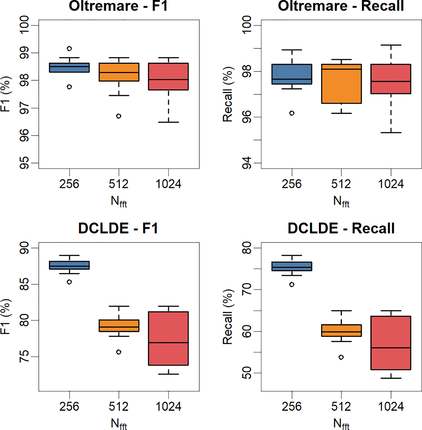
Figure 3. Normalized confusion matrix for Experiment B (five-class Oltremare multiclass demonstration).
Rows represent true classes; columns represent predicted classes. Values are the sum of true-class instances assigned to each predicted class, across the 10 stratified folds. Percentage values, in parentheses, are normalized per row. Diagonal percentage entries correspond to per-class recall.
Lower performance was observed for the Echolocation Click Trains (C3:
) and Burst Pulse Sounds (C2:
). The confusion matrix (Figure 3) provides further insight into these results, revealing significant inter-class confusion between ECT and BPS. To a lesser extent, a similar pattern of misclassification is observable between BPS and Feeding Buzzes.
With the exception of a few cases involving Feeding Buzzes, other vocalizations were rarely misclassified as Whistles. This underlines the high specificity of the Whistle class, likely due to a more refined labeling process and a more distinctive spectral signature in the training dataset.
4 Discussion
4.1 Methodological considerations
In the development of Convolutional Neural Networks (CNNs) for the detection and classification of cetacean vocalizations, an elevate number of signal processing and architectural parameters can impact on the model efficacy. The formal and reproducible parametrization of each experimental trial, coupled with a rigorous evaluation of performance metrics on both in-domain and external datasets, is an improved approach for quantifying the impact of specific data management or model implementation choices.26 The development of a structured pipeline, based on explicit assumptions and standardized protocols, originates from the necessity to address these complexities, providing a reliable toolkit for the systematic optimization of bioacoustic classification models.
Two design choices in these experiments illustrate how the framework supports deliberate, documented decisions. In Experiment A, the negative class was assembled from the full set of non-whistle vocalizations rather than from background noise alone, making the training task harder but more representative of operational conditions. In Experiment B, scroll augmentation was applied selectively to the data-scarce feeding-buzz class, generating sufficient training material without artificially inflating the other classes. Both choices are encoded in the configuration file and reproduce exactly; neither required modifying any code. In a field where preprocessing decisions are often left implicit, recording them in a machine-readable form is itself a methodological contribution.
4.2 Generalization gap and deployment implications
The separation between in-domain and cross-domain results is the central methodological point of Experiment A. In-domain cross-validation alone would suggest a near-solved problem, with a macro F1 of 0.966. The cross-domain evaluation reveals the more realistic figure: the same models recover roughly half the whistles in a genuinely independent recording. A pipeline that stops at in-domain validation would systematically overstate deployment performance; the gap measured here — approximately 21 percentage points of macro F1 — quantifies how large that overstatement can be.
In the dimension that matters most for this detector, the cross-domain result is strong. The false discovery rate was zero across all ten fold models on an entirely unseen dataset, with no inter-fold spread. For an edge-deployed deterrent system, where every false positive triggers an unnecessary intervention, this outcome is preferable to a higher-recall detector with non-zero false alarms.
The framework is what makes this measurement routine. Because every parameter lives in a single configuration file, a practitioner who wants to reduce the generalization gap can modify the training set composition, the spectrogram band, or the class definitions, and re-run only the affected pipeline stages without revisiting annotation or rewriting code. Cross-domain evaluation becomes a standard step of the workflow rather than an exceptional one.
4.3 Limitations
Three limitations bound the scope of these results. First, both experiments use a single species (T. truncatus) and a single training site (Oltremare); the pipeline is designed to generalize through reconfiguration, but that generalization is asserted rather than demonstrated here. Second, the cross-domain test for Experiment A uses one DCLDE recording track, which confirms that the pipeline generalizes but does not characterize how performance varies across many independent sites and conditions. Third, the multiclass results (Experiment B) are purely in-domain; the ECT/BPS confusion pattern described in Section 3.4.1 may change substantially on recordings with different signal-to-noise ratios or individual variation. Finally, despite fixed seeds, small run-to-run numerical differences can arise from multi-threaded CPU floating-point operations; exact bitwise reproduction may require fixing the hardware thread configuration in addition to the seed.
5 Conclusions
This study presented ai-pam-pipeline, an open-source six-stage framework that formalizes the complete workflow from raw audio annotation to cross-domain CNN evaluation, with every parameter defined in a single YAML configuration file. Two experiments on Tursiops truncatus vocalizations validated the framework: a binary whistle detector reached a false discovery rate of 0.000 on an independent open-ocean dataset, with a macro F1 of 0.759; a five-class vocalization classifier demonstrated scalability to multiclass tasks, achieving a macro F1 of 0.843 in-domain with scroll augmentation compensating for a data-scarce class. The toolkit is released under the Apache 2.0 license and archived on Zenodo, enabling other groups to reproduce these results exactly and adapt the workflow to other species or monitoring contexts through configuration alone. The framework was developed within the LIFE DELFI project as infrastructure for operational edge-deployed deterrent systems, and is offered to the wider PAM community as a foundation for reproducible, comparable detector development.
Ethics and consent
Ethical approval and consent were not required for this study. The acoustic recordings used in the experiments were collected as part of the LIFE DELFI project (LIFE19 NAT/IT/000942) and are publicly available. Data acquisition was conducted entirely in passive mode: a hydrophone recorder was positioned unobtrusively within the facility, out of direct view of the animals, and no interaction with, handling of, or intervention upon the recorded individuals took place at any stage. The dolphins were free-swimming in their normal environment throughout the recording sessions. No animal experimentation, invasive procedures, or behavioral manipulation of any kind were performed.
Software Implementation and CLI Usage
The following ten steps reproduce Experiment A (binary whistle detection,
) from a clean system with no prior installation. Estimated time: 15–20 minutes for installation and dataset preparation; training time depends on hardware (GPU recommended).
Step 1 — Download the toolkit.
Download the versioned source archive from Zenodo:
https://doi.org/10.5281/zenodo.19860736
Step 2 — Extract and enter the directory.
unzip ai-pam-pipeline-v1.0.zip cd ai-pam-pipeline
Step 3 — Create a virtual environment.
python -m venv.venv source.venv/bin/activate # Linux/macOS


# .venv\Scripts\activate # Windows
Step 4 — Install dependencies.
pip install -r requirements.txt
Core dependencies include TensorFlow, scipy, Pillow, matplotlib, and soundfile. GPU acceleration is available if a CUDA-compatible device is present and the appropriate TensorFlow GPU build is installed (see Section S1).
Step 5 — Download the Oltremare dataset.
Download the annotated Oltremare dataset from SEANOE:
https://doi.org/10.17882/109081
Step 6 — Place audio files.
Copy all.wav recording files into the data/audio/directory:
ai-pam-pipeline/
└── data/

   └── audio/

      ├── 20211120_102109_192.wav

      └── …
Step 7 — Place label files.
Copy the corresponding Audacity label files (.txt) into data/labels/. Each label file must share the same stem as its audio file:
ai-pam-pipeline/
└── data/

   └── labels/

      ├── 20211120_102109_192.txt

      └── …
Step 8 — Run preprocessing (Stages 1–4).
python ai_pam_preprocessing.py conf/binary_cnn.yaml
This command reads the configuration file conf/binary_cnn.yaml, processes all paired audio/label files, and exports segmented spectrogram images to outputs/spectrograms/. A summary report is printed to the console on completion.
Step 9 — Run training (Stages 5–6).
python ai_pam_train.py conf/binary_cnn.yaml -v
Step 10 — Inspect results.
Open the training summary report: outputs/report/train/summary_report.md.
This file contains cross-fold mean ± SD for all metrics, per-fold detail, and a fold-level confusion matrix. Individual.keras model files and _metrics.json records are available in outputs/models/for further analysis or cross-domain evaluation.




