1. Introduction
Electric vehicles (EVs) are increasingly deployed on road networks that combine dense, well-connected corridors with extensive stretches of sparse infrastructure, low traffic flow, and harsh or rapidly changing environmental conditions (Jung et al., 2023). The former basically encompasses motorways, urban areas, and well-connected suburbs, while the latter concerns mountain passes, rural valleys, forest roads, or cross-border links. Road segments that simultaneously combine complex orography, variable micro-climates, and intermittent or absent cellular coverage are termed here challenging segments: on such sparsely connected segments, both safety-critical perception and energy-aware planning become more difficult (Prasad and Gudipalli, 2025). Range information presented to drivers is most often anchored in type-approval cycles such as the Worldwide-Harmonized Light Vehicles Test Procedure (WLTP (United Nations Economic Commission for Europe, 2022)), whose laboratory conditions are known to systematically diverge from real-world EV consumption, with reported gaps of the order of 15–20% on average and substantially larger on demanding terrain or in cold weather (Weiss et al., 2024; Yuan et al., 2024). Micro-climatic phenomena (fog in a valley, ice in shaded curves, sudden snowfall, extreme temperatures) and local terrain (steep grades, tight turns) can degrade on-board sensor performance and invalidate range estimators that rely on standardised cycles or coarse-grained maps (Mao et al., 2025); intermittent connectivity additionally undermines range estimators that depend on cloud services and frequent end-edge-cloud exchanges (Mulpuri et al., 2025). As a result, drivers may receive outdated or over-optimistic information about remaining range and road conditions precisely where mistakes are less forgiving (Ghazali et al., 2025).
Current Vehicle-to-Everything (V2X) and connected-vehicle architectures are largely optimised for urban or highway environments with continuous cellular coverage and high traffic density (Clancy et al., 2024; Wang et al., 2025). In these settings, vehicles can offload perception tasks to the cloud and benefit from dense probe data fed by cooperative perception pipelines (Wan et al., 2025); frequent over-the-air updates and high-capacity downlinks are similarly enabled by wide-area cellular and emerging 6G V2X technologies (Noor-A-Rahim et al., 2022). In contrast, low-coverage segments often fall back to purely on-board intelligence: models are rarely updated once deployed, and any local knowledge acquired by one vehicle (e.g., unexpected ice, wildlife crossings, temporary lane closures) is not systematically shared with subsequent vehicles. Conventional approaches therefore underutilise the potential of V2X to create a local collective intelligence around difficult road sections, and they offer limited guarantees on how perception and energy models evolve over time in such conditions (Maglogiannis et al., 2022).
The V2X system presented in this paper addresses the mentioned gap by introducing a beacon-centric architecture tailored to low-coverage, safety-critical road segments. Instead of assuming continuous wide-area connectivity, a small number of physical beacons are deployed at the entry and exit of the section of interest. Whenever direct line-of-sight between the entry and exit beacons is available, no further infrastructure is required to keep the two endpoints synchronised; otherwise, the link between them is closed by a small chain of intermediate point-to-point repeaters that act purely as backbone relays and do not participate in V2X exchanges with vehicles. The two end beacons maintain reliable backhaul (when available) and act as local hubs for V2X communication, a role increasingly recognised for roadside units in modern intelligent transportation systems (Bilal et al., 2023; Gong et al., 2023). These beacons broadcast up-to-date summaries of road and weather conditions, receive measurements and model updates from vehicles traversing the segment, and coordinate how this knowledge is aggregated and redistributed. In this way, vehicles entering the section can adapt their perception pipelines, driving strategies, and range estimates in advance, while vehicles leaving the section contribute fresh evidence to improve the system for others.
To make this interaction efficient and privacy-preserving, the proposed architecture couples the beacon infrastructure with an edge Artificial Intelligence (AI) and Federated Learning (FL) pipeline. Lightweight time-series and vision models run directly on vehicles and beacons to forecast energy consumption and risk signals and to interpret local perception cues. Rather than streaming raw sensor data, clients participate in FL rounds in which model updates are aggregated first at beacons and, when possible, forwarded to a cloud server. This hierarchical, communication-aware design is well aligned with vehicular non-Independent and Identically Distributed (non-IID) data distributions, intermittent links, and strict latency constraints (Chellapandi et al., 2024; Zhou et al., 2023); the same design enables continuous adaptation of models to terrain, micro-weather, and traffic conditions without exposing raw, potentially sensitive data beyond the local environment (Du et al., 2020; Zhang et al., 2024).
A central focus of the architecture is context-aware range-risk estimation. The system explicitly incorporates segment-level context, including road geometry, micro-weather, pavement state and recent traversal evidence, recognising their strong influence on EV energy consumption and on the reliability of the information available to drivers (He et al., 2024; Weiss et al., 2024). In the proposed architecture, the same beacon mechanism can also disseminate safety-critical perception cues, such as black ice, debris, wildlife or sudden visibility loss. However, the experimental validation reported in this paper focuses specifically on EV range-risk estimation: reducing unexpected range depletion and avoiding over-optimistic final State of Charge (SOC) predictions before a vehicle enters a connectivity-poor section.
The architecture proposed here is developed within the NOUS reference architecture, which provides the roles, agents, and common services on which the deployment is built. Vehicles and beacons are modelled as Data Space Participants (DSPs) instantiated through the NOUS Data Agent (NDA), while the regional/cloud backend is conceived as a Data Space Infrastructure Provider (DSIP) instantiated through the NOUS Infrastructure Agent (NIA); identity, authorisation, governance, and discovery are delegated to the NOUS common services (
Table 1). This alignment follows the broader principles of sovereign data spaces, in which participants retain control over their data and policy-driven sharing replaces centralised data lakes (Jarke et al., 2019; Otto, 2022).
Table 1. System components instantiated by the beacon-centric V2X/FL system: roles, agents, and responsibilities of each component within the NOUS reference architecture.
| Component | Role | Agent | Responsibility |
|---|
| Vehicle (on-board inference + FL client) | DSP | NDA | Keeps raw data locally; performs inference; produces evidence summaries and FL updates; publishes/consumes data/services under policy control. |
| Entry/Exit Beacon (local hub + mini-aggregator + broadcast) | DSP (opt. DSIP) | NDA (opt. NIA) | Aggregates updates locally (hierarchical FL); disseminates alerts/summaries; optionally exposes edge compute/network as managed infrastructure. |
| Intermediate Repeater (connectivity relay) | DSIP | NIA | Provides policy-aware networking/relay and connectivity between far-edge and regional/cloud resources. |
| Regional/Cloud Backend (sync + model/artifact repository) | DSIP | NIA | Hosts model/artifact repositories; optional higher-capacity aggregation/analytics; provides infrastructure/platform services for deployment and synchronisation. |
| Identity, Authorisation, Governance | Common Services | — | Identity and Access Management (IAM), certification/attestation hooks, policy decision/enforcement points, and service gateway for controlled access. |
| Discovery (agents/apps/models) | Common Services | — | Registries/catalogues enabling discovery of participants, services, and reusable applications. |
| Federated Learning support | DSP + Common Services | NDA | FL orchestration and lifecycle at participant level (NDA), complemented by cross-space coordination services when needed. |
Within this context, the contributions of this paper are threefold:
• A beacon-based V2X architecture for low-coverage road segments is proposed, integrating on-board sensing, roadside context probes, and reliable edge nodes at the section boundaries. The design supports both safety-oriented alerts and energy-aware planning while remaining deployable in infrastructure-scarce environments.
• An edge AI and federated learning pipeline is designed to treat vehicles and beacons as FL clients, support hierarchical and asynchronous aggregation, and incorporate communication-efficient and privacy-preserving mechanisms. The pipeline is tailored to EV energy prediction and risk-aware perception under non-IID, spatio-temporally evolving data.
• Through a digital-twin evaluation of a real mountain-pass segment, the proposed system is shown to reduce route-level range-estimation error and, more importantly, false-safe autonomy decisions when compared with generic or non-local estimators. Communication-layer and perception-layer KPIs are identified as future deployment targets.
The remainder of this article is organised as follows. Section 2 reviews the state of the art in sensing and context modelling, edge AI, federated learning, V2X communication, embedded hardware, and grade- and weather-aware energy estimation. Section 3 presents the proposed V2X architecture, detailing the beacon deployment, data flows, learning protocols, and implementation choices. Section 4 reports the experimental setup and main results, and Section 5 discusses the implications and limitations of the proposed approach and outlines directions for future work.
2. State of the Art
The proposed beacon-centric V2X and federated learning architecture for low-coverage road segments draws on advances in seven complementary research areas. The first concerns sensing and context inputs that feed both perception and energy models; the second and third deal with edge AI for immediate inference and with federated learning protocols suitable for vehicular networks. The fourth pillar is the V2X communication substrate that determines how information actually flows between vehicles, beacons, and the cloud, while the fifth focuses on the embedded hardware that must execute models within strict thermal and latency envelopes. The sixth area gathers the literature on terrain, weather, and environmental factors that drive electric-vehicle energy consumption and dictate the difficulty of any range estimator. The final pillar collects the datasets, simulators, and benchmarks needed to evaluate such systems reproducibly. This section is aimed at reviewing each of these pillars. The experimental contribution of the present paper focuses on the energy and range-risk branch of this architecture; perception, communication-latency and embedded-hardware KPIs are discussed as deployment requirements but are not measured in the current experimental batch.
2.1. Sensing and context inputs
A connected vehicle approaching a low-coverage segment relies on a heterogeneous mix of on-board, roadside, and geospatial signals. On-board sensing typically combines a camera, LiDAR (Light Detection and Ranging) or radar suite with inertial and satellite navigation and with vehicle-bus telemetry such as speed, torque, state of charge, and auxiliary power draw. Recent multi-modal perception studies show that combining these modalities is essential for reliable scene understanding, especially under adverse weather and low illumination, but they also highlight that on-board perception alone degrades in occluded or cluttered environments and benefits substantially from cooperative sources of evidence (Wan et al., 2025; Xu et al., 2023). Roadside and beacon signals complement vehicle telemetry with measurements of temperature, humidity, pavement wetness, micro-weather, infrastructure vibration, and traffic counts; cooperative perception datasets that include infrastructure-mounted sensors confirm that such signals improve detection range and reliability in vehicle-infrastructure scenarios (Yu et al., 2022).
Geospatial context is equally important. Digital Elevation Models (DEMs), grade and curvature profiles, lane geometry, and segment topology are needed to interpret on-board signals at the level of individual road links. High-definition map pipelines now routinely fuse DEMs with vector road geometry, performing semantic and geometric annotation, lane-level segmentation, and topology extraction prior to deployment (Bao et al., 2023). The corresponding data-preparation chain in the present setting includes time-and-space alignment of heterogeneous streams, map matching of Global Navigation Satellite System (GNSS) traces, segmentation of road links, and outlier filtering, which are well-established preprocessing steps in vehicular sensor fusion (Wan et al., 2025).
A recurring theme across this literature is the trade-off between raw data and lightweight evidence summaries. Streaming raw sensor data over a constrained backhaul is rarely feasible in low-coverage contexts, so beacons and vehicles must instead exchange compact descriptors, such as event flags, statistical summaries, model updates, that preserve the relevant information while respecting bandwidth budgets at the edge (Gong et al., 2023); model-update exchanges further protect privacy by keeping raw data on the vehicle and the beacon (Du et al., 2020).
2.2. Edge AI models for immediate inference
For immediate decisions under limited connectivity, models must be both data-efficient and hardware-efficient. Two complementary families dominate: compact time-series predictors for energy/risk signals and lightweight vision backbones for scene cues, with both ultimately compressed and distilled to run on in-vehicle Electronic Control Units (ECUs) or roadside beacons (H.-I. Liu et al., 2024).
On the energy side, recent EV studies have moved beyond purely physics-based estimators towards data-driven predictors that ingest short windows of speed/acceleration, grade, temperature, and auxiliary loads. Large comparative evaluations in 2025 Scientific Reports show that gradient-boosted trees and light neural regressors can outperform legacy baselines for EV energy prediction when trained on real telemetry, highlighting the competitiveness of tabular learners (XGBoost/LightGBM) under tight latency and memory budgets (Hussain, Ching, Uttraphan, Tay, and Noor, 2025a; Hussain, Ching, Uttraphan, Tay, Noor, and Memon, 2025b). In these works, accuracy is reported with Mean Absolute Error (MAE)/Mean Absolute Percentage Error (MAPE) and Root Mean Square Error (RMSE) over trips or segments, and practical gains come from feature engineering that makes road grade and micro-weather explicit, which maps well to the beacon setting considered here, where such context is available locally (He et al., 2024).
Neural time-series models remain attractive when temporal dynamics must be learned directly on the edge. Temporal Convolutional Networks (TCNs) provide long receptive fields through dilations with fewer parameters than recurrent models, making them strong candidates for embedded inference; current surveys emphasise their efficiency and stability for forecasting tasks, where evaluation typically couples MAE/MAPE with horizon-wise error profiles to expose degradation at longer look-ahead times (Kong et al., 2025; Torres et al., 2021). Emerging edge-sized transformers extend this line, and domain-specific architectures such as an Energy Consumption Transformer for EVs indicate that attention mechanisms can capture heterogeneous, non-IID operating regimes (e.g., climbs vs. descents) when modest model sizes are affordable (Huang et al., 2025); the corresponding ablations usually relate error reductions to parameter count and window length, of direct relevance when setting beacon memory budgets (Ngo et al., 2025).
When perception cues matter, such as detecting low-friction surfaces, pooled water, or lane-level context, compact Convolutional Neural Networks (CNNs) remain the workhorse. Comparative studies through 2025 find MobileNetV3 and EfficientNet-Lite/V2 to offer the best accuracy-throughput trade-offs on edge Systems-on-Chip (SoCs), while SqueezeNet-class models excel when footprint and cold-start are dominant (H.-I. Liu et al., 2024). Inference quality is commonly measured with mean Average Precision (mAP)/F1, but for edge deployment the decisive metrics are end-to-end latency and energy per inference (reported in milliseconds and joules); both improve further with early-exit networks that terminate computation once confidence thresholds are met (Rahmath P et al., 2024). These multi-exit designs are particularly useful on beacons that must broadcast within strict deadlines while running from limited power.
Across modalities, the deployment path converges on TinyML techniques: post-training quantisation to int8 or lower, structured/unstructured pruning, and knowledge distillation from a richer cloud model into a compact student that lives on the vehicle or beacon (Somvanshi et al., 2025). The edge-inference literature documents sizeable latency and energy gains from the combination of quantisation-aware training, pruning, and hardware-aware neural architecture search, with negligible accuracy loss when distillation is used (Chitty-Venkata et al., 2023); reported speedups are accompanied by retained accuracy deltas (Δ% top-1 or ΔMAE) and energy savings on representative Neural Processing Units (NPUs)/Central Processing Units (CPUs) (Ngo et al., 2025). This forms the basis for a practical toolchain in the present setting, training centrally on pooled data when available, distilling to small students, then continuing on-device fine-tuning through federated rounds (Chellapandi et al., 2024).
Finally, running models where the data originates is now standard in vehicular edge architectures. Contemporary V2X frameworks and Roadside Unit (RSU)/roadside-edge studies argue for placing perception and forecasting models at the network edge to meet tight latency budgets (Gong et al., 2023); the underlying edge Deep Neural Network (DNN) inference techniques that make such deadlines achievable on resource-limited hardware are catalogued in recent reviews (Ngo et al., 2025). Reported evaluations often pair task metrics with system-level measures such as time-to-alert and packet-loss-robust latency. These metrics are relevant to the full deployment, but the present experimental batch reports only route-level energy and range-risk indicators. In short, the state of the art supports a pipeline in which compact predictors estimate energy/risk on local signals and are then updated through federated mechanisms, which are detailed next (McMahan et al., 2017).
2.3. Federated learning for vehicular edge
In vehicular edge settings with intermittent connectivity, vehicles and beacons are treated as FL clients, with beacons also acting as mini-aggregators when backhaul is scarce. The canonical baseline remains FedAvg, averaging local updates in rounds and establishing the modern FL paradigm of training where data stays local, its convergence and communication behaviour are taken as a reference point for the variants discussed next (McMahan et al., 2017). Building on FedAvg, FedProx adds a proximal term that improves stability under non-IID and system heterogeneity, both unavoidable when different road segments and vehicle types produce skewed data (Li et al., 2020), while SCAFFOLD controls client drift via control variates, often yielding faster convergence for the same communication budget (Karimireddy et al., 2020). In practice, these choices are evaluated not only by final accuracy but by convergence per round and per-round bytes, since these determine how often a beacon must seize scarce spectrum to ship updates. Server-side adaptive optimisers (FedAdam/FedYogi) frequently reduce the number of rounds needed to reach a target error, a property critical when clients are only sporadically reachable (Reddi et al., 2021).
Strict synchrony is fragile on the road, so asynchronous and hierarchical FL are natural design choices for the target deployment. Recent schemes down-weight stale updates, buffer versions, or correct version skew to preserve accuracy when clients connect at random times, which is a natural fit for cars and beacons that communicate only at segment entry or exit points (Lu et al., 2024; Zang et al., 2024). To further localise traffic and reduce backbone pressure, Hierarchical FL (HFL) can be implemented with vehicles pushing updates to a nearby beacon, beacons aggregating locally, and regional/cloud resources synchronising only when available (Gao et al., 2025; Herabad, 2023). Because vehicles and road segments differ, personalised FL is also relevant: parameter-efficient fine-tuning or small client-side adapters can retain a compact global backbone while allowing each vehicle to specialise the model with private state such as payload, degradation or driving style (Yang et al., 2024, 2025).
Communication efficiency is pivotal in this setting. Quantisation schemes such as QSGD reduce payload sizes by orders of magnitude (Alistarh et al., 2017), while sign-based updates such as signSGD push the idea to one-bit gradients (Bernstein et al., 2018); combined with error-feedback, these compressors can approach the convergence of uncompressed Stochastic Gradient Descent (SGD), making accuracy per transmitted byte a meaningful design criterion at the beacon. Over-the-air aggregation (AirComp) and quality-aware client selection are also relevant in wireless links shared with safety traffic (Choi et al., 2025; Xiao et al., 2024). These mechanisms are not evaluated in the present digital-twin batch; they are deployment options for reducing airtime once the range-risk learning task has been validated.
Trust and safety complete the picture. Byzantine-robust aggregation via coordinate-wise median or trimmed-mean mitigates poisoned or faulty clients with provable statistical guarantees (Yin et al., 2018), and trust-bootstrapped rules such as FLTrust extend this protection to more aggressive adversaries (Cao et al., 2021). Secure Aggregation protects client updates in transit such that only their sum is revealed (Bonawitz et al., 2017), and Differentially Private SGD (DP-SGD) bounds information leakage from any single participant at the cost of utility loss (Abadi et al., 2016). In the present paper, these mechanisms are considered deployment requirements for a future field implementation rather than evaluated components. The experimental focus is restricted to range-risk accuracy, false-safe decisions and the feasibility of the vehicle-as-client, beacon-as-aggregator learning workflow. Finally, V2X deployments must align with Public Key Infrastructure (PKI)-based credentialing (IEEE 1609.2/ETSI TS 103 097), including pseudonymous certificates and replay protection for beacon-vehicle messages (ETSI Technical Committee ITS, 2017).
2.4. V2X communication substrate
The communication substrate of a beacon-centric V2X deployment must reconcile two competing needs: ultra-low-latency dissemination of safety alerts and best-effort delivery of bulkier model updates and telemetry. Three families of technologies dominate the design space. IEEE 802.11p/Dedicated Short-Range Communications (DSRC) and its European counterpart ITS-G5 provide ad hoc, decentralised vehicle-to-vehicle and vehicle-to-infrastructure links with deterministic medium access and low latency at short range, while cellular V2X (C-V2X) over the PC5 sidelink and over the Uu interface offers higher capacity, scheduled transmissions, and integration with operator networks. Comprehensive surveys of wireless V2X access conclude that no single technology dominates in all regimes (Clancy et al., 2024): experimental deployments on real highways have shown that C-V2X PC5 generally extends communication range, whereas IEEE 802.11p tends to deliver lower latency in low-density scenarios (Maglogiannis et al., 2022). The advent of 5G New Radio (NR) V2X and the longer-term 6G roadmap promise sub-10 ms latencies, flexible numerologies, and tight integration with edge computing, but require either dense base-station coverage or sophisticated sidelink resource allocation, precisely what is missing on low-coverage segments (Noor-A-Rahim et al., 2022).
The communication patterns relevant to the beacon-centric architecture proposed here follow naturally from these technologies. Beacons broadcast safety-critical summaries and alerts locally, exploit opportunistic uplinks to aggregators when backhaul is available, and rely on store-carry-forward and gossip-style dissemination among neighbouring beacons to bridge connectivity gaps. Recent work on beacon-oriented emergency message dissemination demonstrates that cluster-based broadcast schemes can substantially improve coverage and packet delivery on sparse highway scenarios (Bilal et al., 2023). Quality-of-Service (QoS) management is equally critical: safety messages must be prioritised over background federated-learning traffic, and channel access must respect duty-cycle and congestion-control constraints to avoid degrading the cooperative perception channel during peak load. Edge-intelligence surveys further argue that placing inference and aggregation at the network edge is necessary to satisfy these QoS budgets, since round-trips to a distant cloud cannot meet the deadlines of cooperative warnings (Gong et al., 2023).
2.5. Edge/Embedded hardware
The hardware substrate of a beacon-centric V2X deployment spans two heterogeneous tiers. In-vehicle compute is increasingly dominated by automotive SoC families that integrate Graphics Processing Units (GPUs) and dedicated neural processing units alongside heterogeneous ARM and x86 cores, with platforms in the NVIDIA Drive, Qualcomm Snapdragon Ride, NXP, Renesas, and TI families competing on Tera Operations Per Second (TOPS) per watt and on certifiable real-time behaviour. Recent surveys of edge intelligence in intelligent transportation systems (Gong et al., 2023), complemented by reviews of on-device deep-learning inference in resource-limited environments (Ngo et al., 2025), document that NPU-class accelerators are now able to sustain perception and forecasting workloads with sub-50 ms latency while remaining within strict thermal envelopes, provided that models are appropriately compressed. At the roadside tier, beacons and RSUs typically rely on rugged ARM or x86 edge boxes augmented with lightweight NPUs or Tensor Processing Units (TPUs), such as Coral, Hailo, ARM Ethos-U class, that allow continuous inference on power budgets compatible with solar or grid-tied installation (Somvanshi et al., 2025).
The deployment toolchain converges around standard inference runtimes. ONNX Runtime, NVIDIA TensorRT with INT8 quantisation, Apache TVM, and Intel OpenVINO are routinely used to compile models trained in PyTorch or TensorFlow into hardware-specific kernels, where transformer-oriented inference toolchains report further gains through coordinated quantisation, pruning, and operator fusion (Chitty-Venkata et al., 2023); comparative studies confirm substantial latency and throughput improvements on embedded targets across DNN families (Ngo et al., 2025). Above the runtime layer, edge containerisation frameworks such as K3s and CRI-O simplify the lifecycle management of perception and federated-learning workloads on beacons, supporting rolling updates and policy-driven deployment. Across both vehicle and beacon tiers, design targets are dictated by the cooperative-perception use case: end-to-end inference within tens of milliseconds, thermal envelopes compatible with passive or limited active cooling, and ruggedisation against the vibration, dust, and temperature ranges typical of unattended roadside installations (Gong et al., 2023).
2.6. Terrain, weather and environmental context for EV energy
Electric-vehicle range cannot be modelled adequately without explicit terrain and weather context. Grade-aware modelling exploits DEM-derived slope and curvature profiles, elevation accumulation per segment, and lane-level geometry to capture the asymmetric energy footprint of climbs and descents, including the partial recovery offered by regenerative braking. Empirical studies on real road networks confirm that road type and grade strongly modulate the energy demand of battery-electric vehicles, so range estimators that ignore them systematically under- or over-predict consumption on mountain passes and undulating rural roads (Jonas et al., 2022; Weiss et al., 2024). Micro-weather adds a second dimension of variability: ambient temperature, wind, precipitation, and pavement condition jointly determine rolling and aerodynamic resistance and the auxiliary load drawn by cabin heating or air conditioning. Recent multi-perspective analyses of EV energy consumption based on large field data sets identify temperature, driving conditions, and route grade among the most influential factors and quantify their causal contribution to per-trip energy use (He et al., 2024; Mao et al., 2025).
These dependencies also explain why naive range estimators—linear functions of state of charge, simple averages over recent trips, or values inherited from type-approval cycles such as WLTP (United Nations Economic Commission for Europe, 2022) are insufficient for safety-critical planning. Empirical evaluations of EV consumption report systematic divergences between WLTP-declared values and real-world energy use, with average gaps of 15–20% that can grow substantially on demanding orography or in cold weather (Weiss et al., 2024; Yuan et al., 2024). A vehicle that enters a steep, cold, low-coverage segment with an over-optimistic range prediction may exhaust its battery in a location where neither cellular coverage nor charging infrastructure is available. Recent reviews of data-driven and hybrid range models argue for explicit incorporation of grade, weather, and driving-style features, and for the use of machine-learning pipelines that can be retrained as new traversals accumulate evidence (Mao et al., 2025; Prasad and Gudipalli, 2025).
The beacon-centric architecture proposed here is designed to exploit precisely this need by providing the local context and the federated-learning rounds required to keep such models aligned with the actual conditions of each segment.
2.7. Datasets, simulators and benchmarks
Reproducible evaluation of vehicular FL and V2X architectures relies on a layered ecosystem of simulators, datasets, and benchmarks. Microscopic traffic simulation is dominated by SUMO, whose recent releases support large-scale intermodal scenarios, signal control, and direct co-simulation with vehicle dynamics and energy models (Lopez et al., 2018). For sensor-rich autonomous-driving research, CARLA remains the de-facto open simulator, providing flexible sensor suites, weather and lighting control, and hooks for cooperative perception experiments (Dosovitskiy et al., 2017). Synthetic V2V and V2X cooperative-perception datasets such as those built on top of CARLA, together with real-world counterparts including DAIR (Yu et al., 2022)-V2X and V2V4Real (Xu et al., 2023), have become standard testbeds for cooperative 3D detection and tracking under vehicle-infrastructure constraints. EV-specific co-simulation usually combines a traffic simulator with a physics-based or simplified powertrain model that ingests speed, acceleration, grade, and ambient temperature traces to compute energy use along a trajectory (He et al., 2024).
On the federated-learning side, scalable benchmarking platforms such as FedScale provide realistic client distributions, large-scale simulation runtimes, and reference implementations of canonical FL algorithms, and have been extended with vehicular-flavoured partitions that split data by client geography, time, or season to approximate the non-IID conditions encountered on the road (Lai et al., 2022). Surveys of FL in connected and automated vehicles note, however, that grade-aware splits and explicit V2X communication constraints (intermittent links, prioritised safety traffic, bounded duty cycle) are still under-represented in public benchmarks, leaving a clear gap for evaluations that jointly stress federated optimisation, embedded inference latency, and energy-aware range prediction (Chellapandi et al., 2024; Zhang et al., 2024).
Closing this gap is one of the motivations of the present work. The evaluation combines a real mountain-pass scenario with digital-twin EV traversals and simulated federated learning in order to study the energy and range-risk dimension of a deployment regime that is currently under-represented in standard benchmarks.
3. Methods and Materials
The proposed beacon-centric V2X/FL architecture is evaluated through a digital-twin simulation of a representative low-coverage mountain segment. This section describes, in order, the case-study scenario and its justification (Section 3.1), the beacon-centric architecture and its operational protocol (Section 3.2), the digital-twin pipeline that generates the simulation environment (Section 3.3), the simulated fleet and data acquisition workflow (Section 3.4), the energy-estimation methods compared in the experimental evaluation (Section 3.5), and the evaluation protocol with the Key Performance Indicators (KPIs) actually reported in the experimental results (Section 3.6).
The methodology is deliberately scoped to range-risk estimation rather than to the full V2X stack. Communication-layer KPIs (such as event-to-adaptation latency or message overhead) and perception-layer KPIs (such as risk-detection F1-score) are not produced by the present experimental batch; they would require dedicated perception and event-propagation data, an instrumented V2X stack, and embedded hardware measurements, none of which are part of the current digital-twin configuration. These remain as future evaluation targets and are not included in the KPI set of Section 3.6.
3.1. Case study and scenario
Real-world applicability is an essential validation criterion for this type of architecture. The selected scenario is the Puerto de la Quesera mountain pass, located at 1712 m above sea level in the eastern Spanish Central System, within the Ayllón mountain range. The pass uniquely connects two villages separated by approximately 35 km, with sections featuring slopes exceeding 10% and no continuous mobile coverage along the route (
Figure 1, left). The surrounding region has a population density below 0.5/km2 over an area of 269 km2 and is characterised by harsh winter conditions. The combination of complex orography, sparse traffic, micro-climatic variability and absent cellular coverage matches exactly the definition of challenging segment introduced in Section 1.
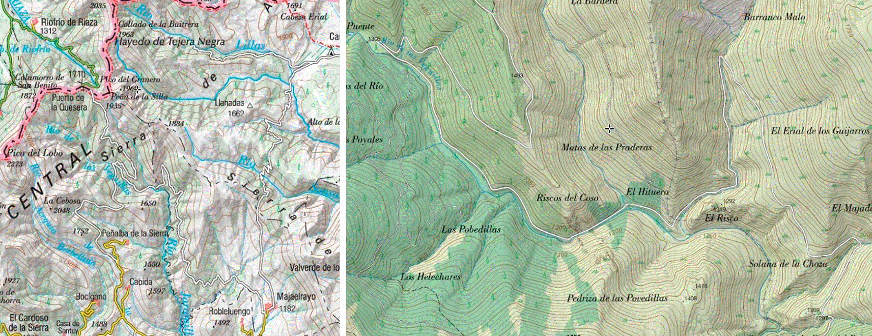
Figure 1. Road sections under study.
Left: Puerto de la Quesera mountain pass road, 35 km from Riofrio de Riaza to Majaelrayo. Right: detail of the 10.6 km segment under study, on the southern side of the pass. Maps extracted and adapted from https://sigpac.mapama.gob.es/fega/visor/.
For tractable simulation, a 10.6 km fragment of the southern flank of the pass was selected (
Figure 1, right;
Figure 2). The fragment is contained within a Digital Elevation Model (DEM) bounding box of approximately 3.86 km × 2.35 km (9.08 km2), covering elevations between 1203 m and 1798 m above sea level (a total relief of 595 m). The fragment was chosen for two reasons: it offers potential line-of-sight between its endpoints, enabling a direct beacon-to-beacon link without intermediate point-to-point repeaters, and it concentrates the orographic and climatic features that make the segment energetically demanding for an Electric Vehicle (EV).
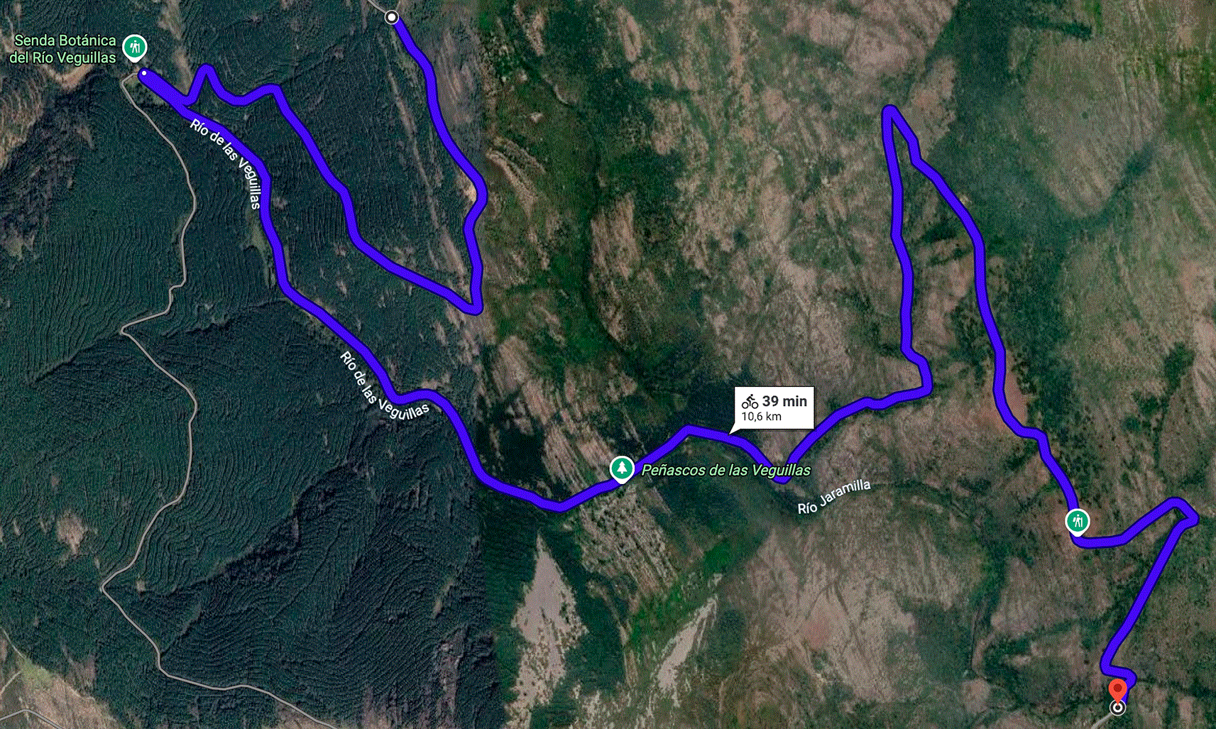
Figure 2. Satellite view of the 10.6 km fragment selected for digital-twin construction.
The serpentine layout, multiple direction reversals and sustained altitude variation make this fragment representative of the most demanding sections of the Quesera pass.
3.2. Beacon-centric architecture and operational protocol
Two physical beacons are deployed at the entry and exit of the segment. Both beacons maintain reliable backhaul to a regional or cloud backend when available, and act as local hubs for V2X exchanges. When direct line-of-sight is feasible between the two beacons, as is the case for the selected fragment, no additional infrastructure is required to keep them synchronised. Otherwise, a small chain of intermediate point-to-point repeaters closes the backbone link without acting as V2X stations themselves; this keeps the certification scope, energy budget, and deployment cost of the intermediate nodes to a minimum.
The operational protocol of the architecture is defined by three interactions between vehicles and beacons.
1.
Pre-entry model delivery. A vehicle approaching the entry beacon receives a compact segment-specific model descriptor before crossing the cellular shadow. This descriptor may include the current residual-model parameters, model version, feature schema, normalisation metadata, recent environmental summaries and any safety-critical alerts contributed by previous traversals. The beacon does not need to compute the final range value for the vehicle; instead, the vehicle evaluates the received model locally using private information such as usable battery capacity, entry SOC, battery state, payload estimate and driver-specific consumption profile.
2.
In-segment local intelligence. Inside the segment, vehicles rely on on-board sensing and on opportunistic Vehicle-to-Vehicle (V2V) exchanges when in range. The architecture does not assume continuous cellular coverage inside the segment.
3.
Post-traversal evidence contribution. When a vehicle reaches the exit beacon, it contributes traversal evidence in the form of a residual model update or compact summary statistics, rather than raw telemetry. The exit beacon aggregates these contributions, synchronises with the entry beacon through the direct or repeater-mediated link, and updates the descriptor that will be served to subsequent vehicles.
This protocol shapes the experimental evaluation in two ways. First, the unit of analysis is the traversal as a whole, because the operational decision to estimate range must be taken before the vehicle enters the segment. Second, the temporal logic of the beacon learning model is prequential: each vehicle is first evaluated with the current beacon model, and only afterwards is its evidence allowed to update the model used for subsequent vehicles. The exact implementation of this protocol in the experimental evaluation is described in Section 3.5.
3.3. Digital-twin pipeline
A digital twin of the selected fragment was constructed to enable controlled, reproducible EV traversals under heterogeneous vehicle and weather conditions. The end-to-end pipeline is summarised in
Figure 3 and described in the following two subsections.
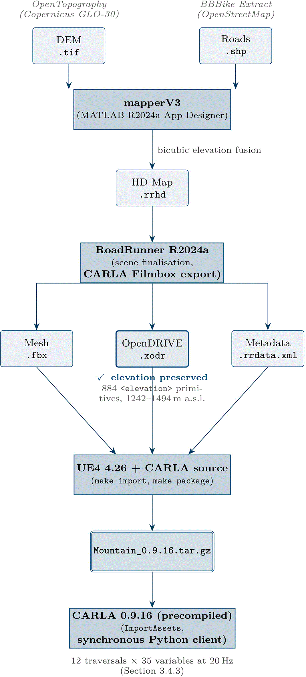
Figure 3. End-to-end digital-twin pipeline used to generate the simulation environment of Section 3.3.
Public Digital Elevation Model and OpenStreetMap road data are fused by the mapperV3 application into a RoadRunner HD Map; the HD Map is finalised in RoadRunner R2024a and exported through the CARLA Filmbox path; the three resulting artefacts are imported into a source build of CARLA on Unreal Engine 4.26 and packaged into the deployable Mountain_0.9.16.tar.gz bundle ingested by the precompiled CARLA simulator at run time. The highlighted.xodr preserves 884 elevation primitives, confirming that the elevation pipeline is not affected by the widespread flat-OpenDRIVE failure mode.
3.3.1. Geospatial preprocessing and HD Map generation
The publicly documented path to bring a real-world road segment into a high-fidelity driving simulator combines a Digital Elevation Model raster and a road centreline vector. The challenging step is to ensure that the lane geometry itself carries the real terrain elevation, rather than running on a flat plane covered by a textured mesh. A widely reported failure mode in the CARLA community is that the exported ASAM OpenDRIVE network (.xodr) ends up with z = 0 in all lanes, which silently invalidates any energy or perception study that depends on real road grade. To address this, a domain-specific desktop application, mapperV2, was developed in the MATLAB App Designer environment (MATLAB R2024a). The application ingests two public inputs:
• GeoTIFF digital elevation model (DEM) tile retrieved from OpenTopography (OpenTopography, n.d.), derived from the Copernicus GLO-30 dataset, with a horizontal resolution of approximately 30 m in the EPSG:4326 coordinate reference system.
• Road-network Shapefile retrieved from the BBBike extraction service from OpenStreetMap data
(OpenStreetMap contributors, n.d.), covering the same bounding box as the DEM tile.
The application then executes the algorithmic pipeline detailed below.
Raster cleaning and reference frame. The GeoTIFF is read with readgeoraster, and no-data sentinel values (entries below −10,000) are replaced with NaN. The local East-North-Up (ENU) origin used by the downstream HD Map is set at the centroid of the DEM bounding box, computed as the mean of the latitude and longitude limits of the raster. This origin is stored as the GeoReference of the generated HD Map and ensures that the local coordinate system is consistent with the geodetic coverage of the input data.
Vector-on-raster elevation fusion. For each polyline in the road Shapefile, the algorithm extracts its (lat, lon) vertices, removes line-separating NaNs introduced by shaperead, and samples the DEM at each vertex using bicubic interpolation through geointerp(…, ‘Cubic’). Vertices whose interpolated elevation is NaN (i.e., outside the DEM coverage) are discarded; polylines that retain fewer than two valid vertices are skipped. Surviving vertices are projected to local metric coordinates using a flat-earth approximation around the ENU origin, and a Gaussian smoother of window length five is applied to the (x, y) traces to suppress OpenStreetMap digitisation noise.
Lane and boundary construction. The smoothed centreline of each road is treated as the lane axis. Forward and backward driving lanes are constructed by offsetting the centreline by ±w_lane/2 along the perpendicular unit normal, with a fixed lane half-width w_lane/2 = 1.75 m. For each road, two roadrunner.hdmap. Lane objects are instantiated (forward and backward) together with three roadrunner.hdmap.LaneBoundary objects (the centre boundary shared by both lanes, plus the two outer boundaries). All geometric entities are populated with full three-dimensional geometry (x, y, z), so that elevation is preserved natively in the HD Map structure. The complete set of lanes and boundaries is assigned to a roadrunnerHDMap object and serialised to a .rrhd
file.
The output of this stage is an HD Map that opens in RoadRunner with the roads already conformed to the terrain mesh, which is the prerequisite for the elevation-aware OpenDRIVE export of the next stage.
3.3.2. Scene finalisation, CARLA export, and packaging
The .rrhd file is opened in MathWorks RoadRunner R2024a. No additional manual editing is required beyond closing the terrain mesh outside the road envelope. The scene is then exported through the CARLA Filmbox export option (File → Export → CARLA Filmbox), producing three artefacts: a .fbx mesh, a .xodr ASAM OpenDRIVE network, and a .rrdata.xml metadata file.
The Filmbox export options used were: Split by Segmentation, Embed Textures, Export Only Highest LODs, and Apply Material Color To Texture. On the ASAM OpenDRIVE tab, the export was configured with OpenDRIVE 1.4, right-hand driving, Enforce connected road continuity, Export signals, Export objects, Export OpenCRG Options with Road Data Format = LRFI. This combination, identified after iterative testing, is the one that preserves the elevation profile of every road inside the .xodr network. Inspection of the exported .xodr file confirms that the elevation profile is non-trivial: the network contains 33 roads with a total of 884 primitives spanning from 1242.4 m to 1493.5 m above sea level. This is the elevation band actually traversed by the road, which lies within the wider 1203–1798 m relief of the DEM tile: the DEM covers the whole surrounding terrain, whereas the .xodr carries only the road centreline elevations.
The three exported artefacts are then dropped into a source build of CARLA 0.9.16 and registered with the CARLA asset pipeline via make import. The map is packaged with make package ARGS = “--packages = Mountain”, producing a deployable bundle that any precompiled CARLA 0.9.16 installation can ingest through the ImportAssets script. The packaged map is referenced internally as Mountain and loaded at run time with the standard CARLA configuration utility (config.py -m Mountain --delta-seconds 0.05). The Unreal Engine version is 4.26.2; no manual edits were performed in the Unreal editor.
Road-grade observation. The exported HD Map preserves elevation in the visual mesh and physics colliders, in the lane geometry of the .rrhd, and in the blocks of the .xodr. However, the elevation field of the navigable waypoint network served by CARLA’s Python API returned z = 0 in the present configuration. To guarantee a physically consistent road grade signal regardless of this limitation, the road grade was derived in real time from the pitch component of the vehicle transform (vehicle.get_transform().rotation.pitch), normalised to the physical range [−90°, +90°]. The pitch-based grade was validated against literature-based predictions of grade-induced energy consumption on equivalent slopes; the agreement justifies the use of vehicle pitch as the working observation of road grade throughout the experimental campaign.
3.4. Simulated fleet and data acquisition
The digital twin was traversed by a heterogeneous simulated fleet under a factorial scenario design. This section describes the EV library, the longitudinal energy model used to derive battery-level variables, the factorial design and the synchronous client-server acquisition.
3.4.1. Electric-vehicle library and longitudinal energy model
Two production EV models were instrumented in the simulator: a Tesla Model 3 RWD (rear-wheel drive) and an Audi e-tron 55 quattro (all-wheel drive Sport Utility Vehicle). Their main parameters, summarised in
Table 2, were taken from manufacturer specifications, EPA test data, the public ev-database, and ADAC tests. Both vehicles were instantiated in CARLA through their native blueprint identifiers (vehicle.tesla.model3 and vehicle.audi.etron, respectively).
Table 2. Parameters of the two EV models used in the simulation campaign.
HVAC stands for Heating, Ventilation and Air Conditioning.
| Parameter | Tesla Model 3 RWD | Audi e-tron 55 quattro |
|---|
| Curb mass (kg) | 1611 | 2490 |
| Drag coefficient Cd | 0.23 | 0.27 |
| Frontal area A (m2) | 2.22 | 2.65 |
| Nominal rolling resistance Crr | 0.011 | 0.012 |
| Nominal pack voltage (V) | 350 | 396 |
| Usable battery capacity (kWh) | 72.0 | 86.5 |
| Motor efficiency η_motor | 0.90 | 0.88 |
| Regen efficiency η_regen | 0.85 | 0.82 |
| Max regen power (kW) | 60 | 220 |
| Max discharge power (kW) | 210 | 300 |
| Internal pack resistance (Ω) | 0.07 | 0.06 |
| HVAC base power (W) | 300 | 400 |
CARLA 0.9.16 does not provide a battery-level electrochemical model. A longitudinal energy model was therefore implemented in Python on top of the kinematic stream produced by the simulator. At each acquisition tick, the instantaneous traction power P_trac required to sustain the observed kinematic state is computed as the sum of four resistive terms plus an auxiliary load, as shown in
Equation (1). For the computation of this equation, the four terms are defined as rolling resistance force F_rr (Equation 2), aerodynamic drag force F_aero (Equation 3), grade or slope resistance force F_grade (Equation 4), and inertial force F_inertia (Equation 5).
(1)
(2)
(3)
(4)
(5)
From
Equations (1)–(5), the variables are defined as follows: v(t) is the longitudinal speed, a_long(t) is the longitudinal acceleration, and θ(t) the road grade inferred from the vehicle pitch angle as a proxy (Section 3.3.2), noting that dynamic effects such as acceleration-induced pitch and suspension dynamics may introduce estimation errors. In addition, m is the curb mass, g is the gravitational acceleration, ρ_air = 1.225 kg/m3 is the air density, and Crr_eff is the effective rolling resistance coefficient after the climatic correction described below (see Section 3.4.2). In addition, Cd is the aerodynamic drag coefficient, A is the vehicle frontal area, and P_aux(t) represents the auxiliary power demand associated with onboard systems such as HVAC, electronics, and other non-propulsion loads.
The instantaneous battery power P_batt(t) (Equation 6) accounts for motor and regenerative braking efficiencies, as well as regenerative and discharge power limits specific to each vehicle, where η_motor is the drivetrain efficiency in traction mode, and η_regen is the efficiency in regenerative braking mode. It is clipped to the interval [−P_regen_max, P_disch_max], where P_regen_max and P_disch_max represent the maximum regenerative and discharge power limits of the battery system, respectively, imposed by the battery and power electronics constraints.
(6)
The state of charge is updated via Coulomb counting, i.e., by numerically integrating P_batt(t) over time and normalising by the usable battery capacity. In addition, cumulative consumed and regenerated energies are tracked separately, ensuring that the route-level net energy demand defined in Equation 7 is well defined and used in Section 4.
(7)
3.4.2. Climate parameterisation and factorial design
Three road-weather conditions were considered, denoted dry24, wet10 and snow_neg5. Each condition is defined consistently across the simulator and the Python energy model.
In CARLA, the conditions are realised by configuring WeatherParameters with the precipitation, surface wetness, wind intensity and sun-altitude values listed in
Table 3. CARLA 0.9.16 does not natively render snow particles; the snow_neg5 condition is therefore not visually distinguishable from a cold overcast scene, and is instead characterised through its physical effects on the EV model, as described next.
Table 3. Climate conditions used in the factorial scenario design.
CARLA-side parameters configure WeatherParameters; model-side multipliers act on the Python energy model.
| Tag | Precip. (%) | Wetness (%) | Wind (%) | Sun alt. (°) | T_amb
(°C) | P_aux (W) | Crr_eff/Crr | η_batt |
|---|
| dry24 | 0 | 0 | 0 | 30 | +24 | 500 | 1.0 | 1.00 |
| wet10 | 60 | 70 | 30 | 10 | +10 | 1500 | 1.2 | 0.95 |
| snow_neg5 | 80 | 40 | 50 | 5 | −5 | 3750 | 2.0 | 0.86 |
On the model side, three climate-dependent multipliers are applied:
1. the auxiliary cabin power P_aux(T_amb) follows a piecewise-linear profile that grows with the deviation from the thermal comfort band (500 W at 24 °C, 1500 W at 10 °C, 3750 W at −5 °C);
2. the usable battery capacity is scaled by a temperature-dependent factor η_batt(T_amb) for Li-ion NMC chemistry: 1.00 at 24 °C, 0.95 at 10 °C, 0.86 at –5 ºC (K. Liu et al., 2018);
3. the effective rolling resistance Crr_eff is scaled by a road-surface multiplier: 1.0 for dry, 1.2 for wet, 2.0 for snow (Sandberg et al., 2011).
The full experimental design is a 2 × 2 × 3 factorial covering two vehicle types, two initial states of charge (SOC) (90% and 40%) and the three climate conditions, for a total of twelve scenarios labelled S01 through S12. The initial SOC factor was included to expose any saturation effect of the regenerative-braking power limit in the prolonged descents of the segment; its effect on the per-traversal net energy is reported in Section 4 and is found to be small in the current simulator configuration.
3.4.3. Synchronous client-server acquisition
Each traversal was executed in CARLA’s synchronous mode with a fixed simulation timestep Δt = 50 ms, corresponding to an acquisition rate of 20 Hz. The simulator acted as a server (Unreal Engine 4.26.2, CARLA 0.9.16) and a Python client coordinated the run: it configured the map, applied the weather parameters of the active scenario, spawned the configured EV at a fixed entry waypoint of the segment, enabled the CARLA Traffic Manager as the autonomous driver, and advanced the simulation one tick at a time. After every tick, the client queried the simulator for the vehicle transform, velocity, acceleration, control inputs and weather state; it then evaluated the longitudinal energy model of Section 3.4.1 and the road-grade observation of Section 3.3.2, and appended a row to the per-traversal Comma-Separated Values (CSV) dataset.
Each row of the resulting dataset contains 35 variables organised in five functional groups: identification and temporality (run identifier, vehicle identifier, simulation timestamp, relative time, time step, OpenDRIVE road and lane identifiers); positioning and topology (pos_x, pos_y, pos_z, road grade in degrees, road curvature, road friction); vehicle dynamics (scalar speed, longitudinal acceleration, lateral acceleration, throttle, brake, steering); battery-level energy variables derived from the longitudinal model (instantaneous battery power, state of charge, pack voltage and current, cumulative regenerated energy, battery temperature); and meteorological state (precipitation intensity, wind speed, road condition category). Each complete traversal of the 10.6 km segment took approximately seven minutes of wall-clock time at a sustained simulation-to-real ratio of approximately 3.2 × .
A representative scenario (S11, Audi e-tron at 40% SOC under wet10) was executed twice under identical configuration to assess the residual stochasticity of the CARLA Traffic Manager. The coefficient of variation of the per-traversal net energy across the two repetitions was below 0.8%, indicating that variability between scenarios reported in Section 4 is dominated by the controlled experimental factors rather than by autopilot noise. The complete dataset, the EV model code and the acquisition script are made available as described in Section 6.
3.5. Energy-estimation methods compared
The evaluation in Section 4 compares generic estimators, a conventional non-local physics estimator, and segment-specific learning methods. The purpose is not to isolate the marginal contribution of a single input variable, but to evaluate whether a model associated with a difficult road segment can reduce route-level autonomy-estimation errors and unsafe range-risk decisions relative to estimators that are not adapted to that segment. The main comparison is therefore between (i) estimators that a vehicle could use without local traversal evidence and (ii) residual models maintained by the beacon from previous traversals.
3.5.1. Generic and non-local baselines
All baselines predict the route-level energy demand Ê_route that a vehicle of a given class will require to complete the 10.6 km segment before entering it. The following baseline methods are taken into account:
•
B0 — Generic nominal estimator. The route energy is estimated as travelled distance multiplied by a vehicle-specific nominal consumption coefficient (Wh/km). This estimator has no access to local traversal evidence and represents a simple range extrapolation.
•
B1 — Conventional non-local physics estimator. The road-load equation (
Equation 1) is integrated along the segment under a generic entry assumption: the vehicle knows its class, nominal parameters and an expected speed profile, but the estimate is not corrected using previous traversals of the target segment. In the implementation used for the reported experiments, this baseline corresponds to the
baseline_entry_flat_wh
column and is the baseline used to initialise the residual model.
Additional physics-only ablations were computed during development to verify the consistency of the simulation pipeline, but they are not reported as main experimental results because the objective of the paper is to evaluate the operational value of segment-specific learning and alert generation.
3.5.2. Centralised segment-specific residual neural model
A residual neural model M1 was trained to predict the residual r(x) between the observed route-level net energy and the conventional non-local baseline estimate, Equation 8; where E_route is the observed (ground-truth) route-level energy and Ê_base is the baseline route-energy estimate available before local correction (the
baseline_entry_flat_wh
output of B1). The network f_θ(x) approximates this residual, with x containing vehicle descriptors, segment descriptors, environmental descriptors and baseline-estimator outputs.
(8)
The corrected route-energy prediction is obtained by adding the learned residual back to the baseline estimate, Equation 9, so that Ê_route ≈ E_route when the residual is predicted accurately.
(9)
The model is trained centrally on pooled traversal data and serves as a reference for the federated and prequential variants. Numeric features are standardised using statistics fitted on the training clients only, categorical variables (vehicle type and road condition) are one-hot encoded, and the target is the segment-level residual with respect to the baseline. The final route prediction is obtained by summing segment-level predictions along the full route.
The residual model is a lightweight Multi-Layer Perceptron (MLP) with three hidden layers of 64, 64 and 32 units, respectively, ReLU activations, no dropout, and a linear output. The final layer is initialised to zero so that an untrained model predicts a zero residual and therefore behaves exactly as the baseline. This avoids leaking the average residual of future vehicles into the cold-start beacon evaluation. Training uses mean-squared error loss and the Adam optimiser.
3.5.3. Federated residual neural model
The federated variant M2 preserves the residual architecture of M1 but trains it through federated aggregation across the twelve traversals, treating each traversal as one client. Two aggregation rules are evaluated, FedAvg (McMahan et al., 2017) and FedProx (Li et al., 2020), with the latter expected to be more stable under non-Independent and Identically Distributed (non-IID) client data. This non-IID setting is natural here because traversals differ in vehicle class, climate condition and initial SOC. Federated training was implemented with Flower (Beutel et al., 2020) using the flwr [simulation] package in the 1.x API range (> = 1.8,<2.0).
3.5.4. Prequential beacon learning
The prequential variant M3 implements the operational protocol of Section 3.2. Traversals are presented to the beacon model in a random arrival order. For each arriving traversal, the current beacon model is first used to estimate Ê_route before the vehicle enters the segment; the prediction error is then measured against the observed E_net; and only afterwards is the traversal allowed to update the beacon model. The update is applied either immediately (aggregation batch size of one) or after a fixed number of arrivals have accumulated (aggregation batch sizes of two and four were also evaluated). The protocol therefore enforces the same temporal causality that would apply in the field: a vehicle benefits only from the experience of previously crossed vehicles. Fifty independent random arrival permutations were generated, and the per-step error was averaged across permutations. The resulting learning curve is the central outcome of the beacon evaluation.
Two aggregation rules are evaluated within M3, mirroring M2: FedProx and FedAvg. The remaining neural and optimisation hyperparameters match those reported in
Table 4. Flower-based replays were used to verify that the vehicle-as-client and beacon-as-aggregator workflow can be implemented with standard FL tooling; the primary statistical evidence reported in Section 4 is provided by the route-level cross-validation results and by the prequential beacon learning curve.
Table 4. Main neural and federated-learning hyperparameters used in the reported experiments.
| Component | Value |
|---|
| Residual model | MLP with hidden layers [64, 64, 32], ReLU activations, linear output, dropout 0.0, zero-initialised final layer |
| Feature set | Segment-entry and local descriptors: distance/position summaries, elevation and grade summaries, curvature, ambient temperature, precipitation, wind, SOC, usable capacity, battery temperature, expected speed, baseline estimates, vehicle type and road condition |
| Target | Segment-level residual with respect to
baseline_entry_flat_wh
; route-level energy obtained by summing segment predictions |
| Optimiser and loss | Adam, mean-squared error loss |
| Batch size | 32 |
| Learning rate and weight decay | 10−3 and 10−5 |
| Centralised training | 200 epochs for the default split; 160 epochs in cross-validation; early stopping patience 30 and 25, respectively |
| Local FL training | 5 local epochs in the main federated/prequential runs; 3 local epochs in cross-validation/checkpoint runs |
| Federated aggregation | FedAvg and FedProx; all available clients participate in each simulated round; FedProx proximal coefficient μ = 0.01 |
| Flower configuration | 12 rounds in the default run; 8 rounds in Flower checkpoint experiments; fraction_fit = 1.0, fraction_evaluate = 1.0, minimum fit clients 2 |
| Prequential evaluation | 50 random arrival permutations; aggregation batch sizes 1, 2 and 4; main tables report immediate updating after each vehicle |
| Random seed | 42 |
3.6. Evaluation protocol and Key Performance Indicators
This subsection defines how the simulation output is turned into quantitative evidence: the unit of evaluation and data splits, the regression and risk-oriented Key Performance Indicators (KPIs) actually reported in this work, and the broader architectural KPIs deferred to future evaluation.
3.6.1. Unit of evaluation and data splits
The unit of evaluation is the complete traversal of the segment, not an individual simulator tick or sub-segment. This choice matches the operational use case described in Section 3.2: a vehicle approaching the entry beacon must estimate, before entering the segment, how much energy will be required to complete the section. Although each traversal also produces sub-segment information (the twelve traversals decompose into 1,212 road sub-segments covering 119.94 km of cumulative simulated driving), no claim is made about per-sub-segment prediction accuracy.
Five cross-validation protocols are used to characterise the residual model under different distribution-shift assumptions:
•
Leave-one-route-out (LORO): each traversal is held out in turn while the remaining eleven are used for training. This is the standard within-distribution evaluation.
•
Leave-one-scenario-group-out: traversals sharing the same combination of vehicle and climate are held out together. This evaluates generalisation to a previously unseen operating regime of the same fleet.
•
Repeated random client split: repeated random partitions of the twelve traversals into train and test subsets, averaged over multiple seeds.
•
Leave-one-weather-out: all traversals under a given climate condition are held out simultaneously. This is a deliberate out-of-distribution stress test.
•
Leave-one-vehicle-out: all traversals of one of the two vehicle classes are held out simultaneously. This is a second deliberate out-of-distribution stress test.
The prequential evaluation of M3 uses its own temporally-ordered protocol, as described in Section 3.5.4, and is therefore not part of the cross-validation table.
3.6.2. Regression KPIs
For every method and every traversal, four regression KPIs are computed and aggregated across traversals.
•
MAE (kWh). Mean absolute error between predicted and observed route-level net energy. Reported as the mean of per-traversal absolute errors, with the standard deviation across traversals as the dispersion measure.
•
Bias (kWh). Signed mean error. A negative bias indicates systematic underestimation of the required energy, which is the safety-relevant failure mode in the present setting.
•
MAPE (%). Mean absolute percentage error. Useful to compare methods on a relative scale across vehicle classes that differ in absolute energy demand.
•
Final-SOC MAE (% SOC). Mean absolute error of the predicted final state of charge against the observed final state of charge. This KPI translates the energy error into the SOC margin that is actually displayed to drivers and used by range-anxiety mitigation logic.
3.6.3. Risk-oriented KPI and alert-generation logic
Average regression error is not sufficient to evaluate the proposed system, because the operational cost of an error is asymmetric. In a low-connectivity mountain segment, an over-optimistic prediction is more critical than a conservative one: a vehicle that is wrongly told that it can safely cross the section may reach the exit with insufficient reserve, whereas a conservative warning mainly produces inconvenience or a detour recommendation. For this reason, the evaluation includes an alert-oriented KPI set in addition to MAE, MAPE and bias.
For each route-level prediction, the estimator outputs the expected energy required to complete the segment, Ê_route. Given a simulated entry state of charge SOC_in and the usable battery capacity C_use, the predicted final state of charge is computed following Equation 10. The observed final state of charge is computed analogously from the measured route-level net energy E_net as stated by Equation 11.
(10)
(11)
A minimum reserve threshold σ_rsv = 5% SOC is fixed. The predicted alert decision is then defined by Equation 12, where  = 1 means that the system issues a low-reserve alert before the vehicle enters the segment. The true risk state could be computed by Equation 13.
(12)
(13)
The alert evaluation is therefore a binary decision problem derived from the energy-estimation task. A false-safe decision occurs when  = 0 and A = 1: the system does not issue an alert, but the vehicle actually finishes the segment below the reserve threshold. This is the primary safety-relevant failure mode. A false-warning decision occurs when  = 1 and A = 0: the system issues an alert, but the vehicle would have completed the segment above the reserve threshold. False warnings are undesirable because they may reduce user trust, but they are less critical than false-safe decisions.
The following risk-oriented metrics are reported:
•
False-safe rate: fraction of route-SOC decisions in which the estimator fails to warn despite the actual final SOC being below the reserve threshold.
•
False-warning rate: fraction of route-SOC decisions in which the estimator warns despite the actual final SOC being above the reserve threshold.
•
Risk recall: fraction of truly risky cases correctly detected by the estimator.
•
Alert precision: fraction of emitted alerts that correspond to truly risky cases.
The false-safe rate is treated as the primary risk KPI. A model is considered operationally better when it reduces false-safe decisions without producing an excessive number of false warnings. This criterion reflects the intended role of the beacon: not to provide an exact battery forecast in all conditions, but to prevent unsafe over-confidence before entering an isolated and energetically demanding segment.
3.6.4. Architectural KPIs as future evaluation targets
The KPI set above is restricted to energy estimation and range-risk decisions, which are the outcomes that the present experimental campaign actually produces. Architectural KPIs that would characterise the deployed beacon-V2X-FL system as a whole, including event-to-adaptation latency, on-vehicle adaptation time, risk-detection F1-score, risk-mitigation rate, no-update gap, stale-context fraction, and power-consumption overhead, require dedicated perception data, an instrumented V2X communication stack, and measurements on representative embedded hardware. They are therefore not reported in Section 4 and are explicitly stated as future evaluation targets. Their definition and the corresponding instrumentation are sketched in the discussion (Section 5).
4. Results and Analysis
This section evaluates the proposed beacon-centric V2X/FL architecture as a local range-risk estimation mechanism for a low-connectivity mountain-road segment. The purpose of the evaluation is not to isolate the contribution of any single physical input, but to determine whether a segment-specific model, learned from previous traversals and distributed through roadside beacons, can reduce over-optimistic range decisions before an EV enters a demanding section.
The evaluation is organised around four research questions:
•
RQ1: How variable is the energy demand of the selected segment across vehicle and road-weather conditions?
•
RQ2: Does a segment-specific model reduce route-level energy-estimation error and unsafe over-optimistic (false-safe) decisions relative to generic or non-local estimators?
•
RQ3: How robust is the residual model under route-level cross-validation and distribution-shift protocols?
•
RQ4: Does the prequential beacon protocol reduce unsafe over-optimistic decisions as more vehicles traverse the segment?
The results reported here are restricted to energy estimation and range-risk assessment. Communication-layer and perception-layer KPIs, such as event-to-adaptation latency, risk detection F1-score and risk mitigation rate, require dedicated perception and V2X instrumentation and are therefore left for future work.
4.1. Route-level energy variability
As it was previously stated, the evaluation was conducted on 12 simulated traversals of the selected 10.6 km mountain segment. Each traversal is treated as one vehicle-client in the federated-learning setting. The simulated fleet comprises two EV models, a Tesla Model 3 and an Audi e-tron, under three road-weather conditions: dry pavement at 24 °C, wet pavement at 10 °C, and snow/low-temperature conditions at −5 °C. Two initial SOC levels were considered, 90% and 40%, although the current simulator configuration gives limited influence to initial SOC in the final net energy.
The 12 traversals were decomposed into 1,212 road sub-segments, covering 119.94 km of cumulative simulated driving. The evaluation metric, however, is computed at traversal level. This matches the operational use case: a vehicle approaching the entry beacon must decide, before entering the segment, whether the expected energy requirement leaves enough reserve at the exit.
Table 5 summarises the observed net energy demand. The same road segment requires substantially different energy depending on vehicle class and road-weather condition. For the Tesla Model 3, the route energy increases from approximately 1.68 kWh in dry conditions to approximately 3.35 kWh in snow. For the Audi e-tron, the corresponding range is approximately 2.82 kWh to 4.63–4.67 kWh. This variability supports the need for a local segment-specific model: the relevant quantity is not merely the distance to be travelled, but the expected energy demand of this particular section under its current operating conditions.
Table 5. Observed net energy demand for the simulated mountain-segment traversals.
Values are grouped by vehicle and road-weather condition.
| Vehicle | Condition | Observed net energy demand |
|---|
| Tesla Model 3 | Dry, 24 °C | ≈ 1.68 kWh |
| Tesla Model 3 | Wet, 10 °C | ≈ 2.09–2.21 kWh |
| Tesla Model 3 | Snow, −5 °C | ≈ 3.35 kWh |
| Audi e-tron | Dry, 24 °C | ≈ 2.82 kWh |
| Audi e-tron | Wet, 10 °C | ≈ 3.14–3.27 kWh |
| Audi e-tron | Snow, −5 °C | ≈ 4.63–4.67 kWh |
4.2. Generic versus segment-specific estimation
The first comparison evaluates whether generic estimators provide sufficient reliability for the selected segment.
Table 6 reports the main route-level results. The nominal-consumption baseline obtains an MAE of 0.777 kWh and a negative bias of −0.777 kWh. The conventional non-local physics baseline obtains a larger MAE of 1.975 kWh and a similarly negative bias. In both cases, the relevant observation is not only the magnitude of the error but its sign: the generic estimators are systematically optimistic and tend to underestimate the energy required to complete the segment.
Table 6. Generic versus segment-specific route-level energy estimation.
Negative bias indicates systematic underestimation of the required energy.
| Method | MAE (kWh) | Bias (kWh) | MAPE (%) | Final-SOC MAE (% SOC) |
|---|
| Generic nominal estimator | 0.777 | −0.777 | 22.67 | 1.12 |
| Conventional non-local physics estimator | 1.975 | −1.975 | 64.48 | 2.71 |
| Segment-specific residual model, LORO | 0.220 | +0.078 | 7.75 | 0.30 |
By contrast, the centralised segment-specific residual model obtains an MAE of 0.220 kWh in leave-one-route-out evaluation. This corresponds to an approximate 71.7% reduction relative to the nominal-consumption baseline and an approximate 88.9% reduction relative to the conventional non-local physics baseline. The result indicates that traversal evidence from the same segment contains useful information for correcting route-level energy estimates.
The largest errors of the generic estimators occur in adverse conditions. Under snow and low temperature, the nominal estimator underestimates the energy required by approximately 1.8 kWh on average. Such a deviation is operationally relevant because, for a vehicle entering the segment with low SOC, an error of this magnitude can determine whether the predicted final SOC remains above or below the reserve threshold. The safety-relevant consequence of this systematic underestimation, i.e. its effect on false-safe range decisions, is quantified in the alert-oriented evaluation of Section 4.5.
4.3. Cross-validation of the segment-specific residual model
The residual neural model was evaluated with route-level cross-validation. Splits were always performed by complete traversal, never by simulation tick or road sub-segment, to avoid leakage between consecutive samples from the same route.
Table 7 summarises the results.
Table 7. Cross-validation results of the segment-specific residual model.
Values are MAE mean ± standard deviation in kWh.
| Protocol |
Residual model MAE (kWh) |
|---|
| Leave-one-route-out
| 0.220 ± 0.164 |
| Leave-one-scenario-group-out | 0.167 ± 0.145 |
| Repeated random client split | 0.231 ± 0.141 |
| Leave-one-weather-out
| 1.228 ± 1.583 |
| Leave-one-vehicle-out
| 1.568 ± 1.150 |
The model performs well when the test traversal belongs to a regime represented in the training set, as shown by the leave-one-route-out, leave-one-scenario-group-out and repeated random split protocols. However, performance deteriorates when an entire weather condition or an entire vehicle type is withheld from training. This behaviour is expected given the small dataset size: 12 traversals, two vehicle models and three weather regimes are sufficient for a proof of concept, but not for training a universal estimator for unseen domains.
This result supports the intended deployment logic. The proposed system should not be interpreted as a static global model trained once and applied everywhere. Its value lies in maintaining a local model for a specific segment and updating it as vehicles traverse that segment under the conditions actually encountered there.
4.4. Prequential beacon learning
The beacon-based setting was evaluated with a prequential protocol. Vehicles arrive sequentially. For each vehicle, the current beacon model is first used to estimate the route energy before entering the segment. The vehicle then completes the traversal, the prediction error is measured, and only afterwards is the traversal allowed to update the beacon model. This protocol enforces the same temporal causality as the field deployment: a vehicle can benefit only from the evidence contributed by previous vehicles.
The learning curve was computed over 50 random vehicle-arrival permutations and different aggregation batch sizes.
Table 8 reports the results for immediate updating after each traversal. With no prior vehicles, the beacon starts from the conventional non-local baseline. As evidence accumulates, FedProx progressively reduces its route-energy error, from 1.975 kWh with no prior vehicles to 0.617 kWh after eight. The trajectory is not strictly monotonic, a transient rise appears at four vehicles and, in average MAE terms, FedProx only overtakes the simple nominal estimator after about eight traversals; with fewer vehicles the nominal estimator remains competitive. The operationally decisive advantage of the beacon appears earlier in the alert-oriented evaluation (Section 4.5), where the false-safe rate is reduced well before the MAE crossover.
Table 8. Prequential beacon learning curve with immediate updating after each traversal.
Values report MAE mean ± standard deviation in kWh over vehicles not yet seen by the beacon.
| Vehicles previously seen | FedProx | FedAvg | Nominal estimator |
|---|
| 0 | 1.975 ± 0.000 | 1.975 ± 0.000 | 0.777 ± 0.000 |
| 1 | 1.602 ± 0.166 | 1.611 ± 0.185 | 0.778 ± 0.067 |
| 2 | 0.860 ± 0.230 | 0.931 ± 0.269 | 0.785 ± 0.103 |
| 4 | 0.951 ± 0.391 | 0.918 ± 0.338 | 0.764 ± 0.132 |
| 8 | 0.617 ± 0.339 | 0.682 ± 0.305 | 0.768 ± 0.315 |
The learning curve indicates that the beacon model is most useful after it has accumulated evidence from several previous traversals. This is consistent with the proposed architecture: the first vehicles provide the initial local evidence, and subsequent vehicles receive progressively better segment-specific estimates. The choice of aggregation batch size affects this process. Updating after every vehicle provides the fastest adaptation, which is attractive for low-traffic roads. Aggregating every two vehicles offers a compromise between responsiveness and client aggregation, while larger batches delay learning and may be less suitable for sparse mountain passes.
4.5. Alert-oriented range-risk evaluation
The operational purpose of the beacon is not only to reduce average error but to prevent unsafe over-confidence. For this reason, the energy prediction was converted into an alert decision using a 5% SOC reserve threshold. For each traversal, eight entry-SOC values were simulated, producing 96 route-SOC decisions. A false-safe case occurs when the estimator predicts that the vehicle will finish above the reserve threshold, but the observed final SOC falls below it.
Table 9 reports the main alert-oriented results. The conventional non-local physics estimator produces 14 false-safe cases, corresponding to a false-safe rate of 14.58%. The nominal estimator reduces this to 8 cases, but still fails to warn in several low-SOC scenarios. The segment-specific residual model reduces the false-safe rate to 1.04% in leave-one-route-out evaluation.
Table 9. Alert-oriented evaluation using a 5% SOC reserve threshold.
Values are computed over 96 route-SOC decisions.
| Method | False-safe rate | False-safe cases | False-warning rate | Risk recall |
|---|
| Conventional non-local physics estimator | 14.58% | 14 | 0.00% | 0.00 |
| Generic nominal estimator | 8.33% | 8 | 0.00% | 0.43 |
| Segment-specific residual model, LORO | 1.04% | 1 | 0.00% | 0.93 |
The prequential beacon model also improves the alert behaviour as more vehicles contribute evidence.
Table 10 shows the evolution for FedProx with immediate updating. With no previous vehicles, the beacon inherits the 14.58% false-safe rate of the initial non-local model. After two previous vehicles, the false-safe rate falls to 5.43%. After eight previous vehicles, it reaches 3.38%. This represents an approximate 60% reduction relative to the nominal estimator and an approximate 76% reduction relative to the conventional non-local estimator.
Table 10. Evolution of false-safe rate as the beacon observes more vehicles.
FedProx with immediate updating is shown.
| Vehicles previously seen | FedProx false-safe
| Nominal false-safe
| Conventional non-local false-safe
|
|---|
| 0 | 14.58% | 8.33% | 14.58% |
| 2 | 5.43% | 8.35% | 14.70% |
| 4 | 3.63% | 8.28% | 14.50% |
| 8 | 3.38% | 8.44% | 14.12% |
This alert-oriented result is the strongest operational evidence in the experiment. Even when the beacon model is not always the best method in average regression error, it reduces the most safety-critical failure mode: telling a driver that the segment can be completed safely when the final SOC actually falls below the reserve threshold.
4.6. Summary of results
The results support three main observations. First, the selected mountain segment produces highly variable energy demand depending on vehicle type and road-weather condition, so generic range extrapolation is insufficient. Second, a segment-specific residual model substantially reduces route-level energy-estimation error when evaluated within the observed distribution. Third, the prequential beacon protocol progressively reduces false-safe decisions as more vehicles traverse the segment, which directly supports the intended use case of range-risk alerting in low-connectivity mountain roads.
5. Discussion and Conclusions
This work proposed and evaluated a beacon-centric V2X/FL architecture for range-risk estimation in low-connectivity mountain-road segments. The central premise is that an EV entering such a segment should not rely exclusively on generic consumption factors or static range extrapolation. The energy required to complete the section depends on the segment itself, the current road-weather condition, the vehicle class, and the recent behaviour observed from previous traversals. The proposed beacon acts as a local holder of this segment-specific knowledge.
The experimental results support this premise. The observed energy demand of the same 10.6 km segment varies substantially across vehicle and road-weather conditions, from approximately 1.68 kWh for the Tesla Model 3 in dry conditions to more than 4.6 kWh for the Audi e-tron under snow and low temperature. Generic estimators do not fully capture this variability. The nominal estimator underestimates the required energy by 0.777 kWh on average, while the conventional non-local physics estimator underestimates it by 1.975 kWh. The sign of the bias is important: the problem is not merely random error, but systematic optimism.
This systematic optimism has direct operational consequences. A route-energy error becomes safety-relevant when it changes the predicted final state of charge from below to above the minimum reserve threshold. For this reason, the study evaluated not only regression metrics but also alert-oriented metrics. The false-safe rate measures the proportion of cases in which the system fails to warn although the actual final SOC falls below the reserve threshold. This is the most relevant failure mode for the proposed application, because a false-safe decision may encourage a driver to enter an isolated segment with insufficient energy margin.
The alert-oriented evaluation shows the practical value of a segment-specific model. The conventional non-local estimator produces a false-safe rate of 14.58%, and the nominal estimator produces 8.33%. The segment-specific residual model reduces this value to 1.04% in leave-one-route-out evaluation. More importantly, the prequential beacon protocol shows progressive improvement as local evidence accumulates. With no previous vehicles, the beacon inherits the initial model and its false-safe rate is 14.58%. After two previous vehicles, the false-safe rate falls to 5.43%; after eight previous vehicles, it reaches 3.38%. Thus, even with a small simulated fleet, the beacon reduces the most safety-critical type of error.
The prequential design is essential to interpreting this result. Unlike a conventional offline evaluation, the beacon model is not allowed to use the current vehicle before predicting for it. Each vehicle benefits only from previous traversals, and only contributes after leaving the segment. This reproduces the causal structure of the intended deployment. The result therefore supports the idea that roadside infrastructure can accumulate local segment knowledge and make it available to subsequent vehicles without requiring continuous cloud connectivity.
The cross-validation results also clarify the scope of the learned model. The residual model performs well when tested on routes drawn from operating regimes represented in the training set, but its error increases under leave-one-weather-out and leave-one-vehicle-out protocols. This limitation is expected given the current dataset size: the evaluation includes only 12 traversals, two EV models and three weather regimes. Rather than invalidating the proposal, this finding reinforces the deployment logic. The model should not be interpreted as a universal estimator trained once and applied everywhere; it should be interpreted as a local, adaptive segment model that improves as vehicles actually cross the section under the relevant conditions.
From an architectural standpoint, the proposed system has three implications. First, the beacon should not simply broadcast a fixed energy value for the segment. Such a value would ignore private vehicle state such as payload, battery degradation, cabin-heating strategy or driver-specific consumption profile. Instead, the beacon should distribute a compact segment-specific model or model update, which the vehicle evaluates locally using its private information. Second, federated learning is justified by the ownership and locality of traversal data: the raw trace remains on the vehicle, while only model updates or compact statistics are shared. Third, the aggregation policy must be adapted to traffic volume. Immediate updating provides fast adaptation for low-traffic roads, whereas larger aggregation batches may provide stronger aggregation but delay usefulness.
Several limitations must be acknowledged. First, the evaluation is based on a digital twin and a longitudinal EV energy model rather than on real vehicle telemetry. Real deployments would introduce additional factors such as tyre pressure, battery ageing, HVAC control strategy, payload, traffic interaction, driver behaviour and manufacturer-specific powertrain control. Second, the number of traversals is small, which limits the statistical strength of the federated-learning comparison. Third, the current experiment evaluates range-risk alerts, not the full V2X/perception stack. Communication latency, packet delivery, power-consumption overhead, perception-risk detection and event-to-adaptation latency require dedicated instrumentation and are left for future work. Fourth, the risk threshold was fixed at 5% SOC; production deployments may require dynamic thresholds depending on distance to charger, outside temperature, vehicle health and driver preference.
To extend the evaluation framework beyond route-level energy estimation and range-risk alerting,
Table 11 defines system-level KPIs for the deployment of the NOUS reference architecture. These KPIs cover communication continuity, context freshness, event-driven adaptation, perception-level risk detection, embedded execution cost and on-vehicle update time. They provide a structured validation roadmap for future deployments of the beacon–V2X–FL architecture.
Table 11. System-level KPIs defined as future evaluation targets for the complete NOUS/V2X deployment.
| KPI | Definition | Required future instrumentation |
|---|
| Section length | Length of the road segment covered by the beacon-based service, including low-coverage areas and any instrumented entry, exit or relay points. | Road-segment survey, beacon placement plan and communication-coverage characterisation. |
| No-update gap | Fraction of the segment in which a vehicle cannot receive a fresh update from a beacon or neighbouring vehicle. | Instrumented V2X communication stack, packet-delivery logs and position-synchronised coverage traces. |
| Stale-context fraction | Fraction of the segment in which the vehicle operates with context information older than the most recent relevant event affecting the section. | Event timestamping, context-version tracking and synchronised beacon/vehicle logs. |
| Event-to-adaptation latency | Time elapsed between the detection of a relevant road or risk event and the moment at which a following vehicle has incorporated the corresponding update into its operational policy. | End-to-end event propagation traces, V2X message logs and on-vehicle adaptation timestamps. |
| Risk-detection accuracy | F1-score or equivalent detection metric for identifying hazardous road-context conditions, such as low friction, obstacles, visibility loss or other perception-level risks. | Labelled perception dataset, validated risk annotations and perception models deployed on vehicles or roadside units. |
| Risk-mitigation rate | Fraction of detected hazardous situations for which the system adapts the vehicle or beacon policy before the affected point is reached. | Joint perception, communication and decision logs linking event detection, policy adaptation and vehicle position. |
| Range-estimation accuracy | Accuracy of the predicted energy demand or final state of charge for completing the segment. | Already evaluated in this paper through route-level energy-error and final-SOC metrics; future work should validate it with real telemetry. |
| Power-consumption overhead | Additional power or energy cost introduced by running the AI, V2X and FL components on the vehicle or roadside edge hardware. | Measurements on representative embedded platforms, including inference, communication and model-update workloads. |
| On-vehicle adaptation time | Time required by the vehicle to apply a received model, context or policy update after reception. | Embedded implementation on an in-vehicle or representative edge device, with update-loading and inference-readiness timestamps. |
Future work should therefore extend the evaluation in four directions. First, the simulation campaign should include additional vehicle classes, payload levels, battery-health states, driving styles and traffic conditions. Second, real or semi-real telemetry should be collected on the selected mountain segment to validate the digital-twin conclusions. Third, the FL protocol should incorporate asynchronous updates, secure aggregation, robust aggregation and update compression, all of which are relevant in sparse vehicular networks. Fourth, the system-level KPIs defined in
Table 11 should be evaluated in an instrumented deployment that includes perception data, V2X communication traces and representative embedded hardware. Finally, the binary alert policy should be extended into graded warnings, for example normal, low-margin and high-risk states, so that the driver receives more interpretable guidance than a single safe/unsafe decision.
In conclusion, the study shows that range-risk estimation on isolated mountain segments benefits from a model that is specific to the segment and updated from recent traversals. Generic or non-local estimators can be systematically optimistic, producing false-safe decisions at low entry SOC. A beacon-centric V2X/FL architecture provides a technically plausible mechanism to reduce this risk: vehicles receive a local model before entering the section, evaluate it with their private state, and contribute updates after completing the traversal. The most important result is not only a reduction in average energy-estimation error, but the progressive reduction of false-safe alerts as the beacon observes more vehicles. This supports the proposed architecture as a privacy-preserving and locally adaptive range-risk mitigation layer for challenging road segments.
Software Availability
The software supporting this study comprises the Python pipeline for preprocessing, baseline computation, residual-model training, Flower-based federated training and prequential beacon evaluation (NumPy, pandas, scikit-learn, PyTorch, Flower, Matplotlib and PyYAML; federated experiments use flwr [simulation] in the > = 1.8,<2.0 range), together with the mapperV3 digital-twin middleware, which is a MATLAB App Designer tool, also distributed as a standalone Windows executable requiring no MATLAB licence, that fuses a GeoTIFF DEM and an OpenStreetMap road network into an elevation-aware RoadRunner HD Map.







