Three methodologies regarding the identification of the model parameters are proposed and their results compared, aiming to keep a high prediction accuracy and at the same time to reduce the computational time needed, when changing the refrigerant. This becomes crucial when there are no data available for a compressor-refrigerant pair. The three methods are highlighted next:
The next sections describe first the complete adapted semi-empirical model, which actually concerns the first method highlighted before once the full set of parameters is included. The second and third method also rely on the same semi-empirical model, once the number of parameters to be optimized are reduced (method 2) or eliminated (method 3).
Description of the adapted semi-empirical model
The original semi-empirical model20 considers four steps to describe the process of the vapour refrigerant inside the compressor and its goal is to predict the following key indicators: the exhaust temperature, the mass flow rate, and the electrical power. The necessary inputs are the supply temperature, the evaporating and condensing pressures, the ambient temperature, and the compressor speed.
Further steps are introduced here, with some inspired by D’Amico et al.23, in order to enhance the physical background of the process also including the pressure drop at the suction and exhaust ports and leaking refrigerant within the compressor. The performance indicators have been defined based on recent practices24 as a function of a set of parameters with physical importance that can be determined from experimental or manufacturer data. The evolution of the refrigerant through the compressor is shown in Figure 1 and consists of eight steps in total.
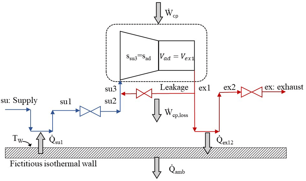
Figure 1. The refrigerant sub-processes within the compressor.
The refrigerant enters the compressor at state 1 (su) and exits at state 8 (ex) with the sub-processes described below and illustrated in the pressure-enthalpy chart of Figure 2.
1. Isobaric heating-up, due to the hot motor and the casing, which are maintained at a higher average temperature than the refrigerant’s suction temperature (su→su1).
2. Supply (adiabatic) pressure drop at the suction port and the motor (su1→su2).
3. Mixing of supply flow with the leakage flow, with the latter undergoing a throttling process which reduces its pressure (su2→su3).
4. Isentropic compression of the refrigerant to the intermediate pressure (su3→ad).
5. Adiabatic compression from the intermediate pressure to the exhaust one (before pressure drop) at constant volume (ad→ex1).
6. Leaking flow to the compressor inlet (ex1→supply line).
7. Exhaust isobaric cooling due to the lower temperature of the fictitious isothermal wall than the exhaust refrigerant (ex1→ex2).
8. Pressure drop at the exhaust port reaching the discharge pressure (ex2→ex3).
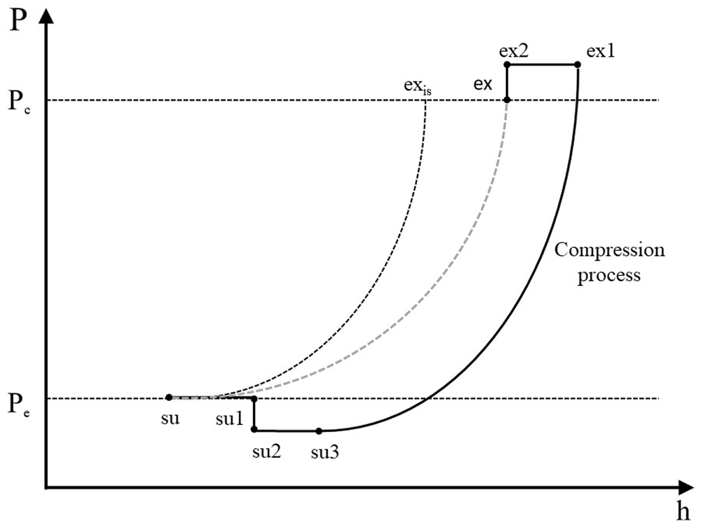
Figure 2. Refrigerant processes during compression in a pressure-enthalpy diagram.
Description of the refrigerant processes during compression. Scroll compressors are volumetric machines and they are characterized by a fixed build-in volume ratio, rv,in, which results to a predefined refrigerant compression up to a certain volume22. For a given refrigerant and operating conditions, there is a unique pressure ratio that corresponds to this volume ratio. Ideally, the compressor should be operated under this pressure ratio, but this is not possible in most cases, because the external (operating) pressure ratio is different than the internal one, leading to either over-compression or under-compression requiring additional power for the process. This diversion from the ideal compression is modeled by splitting the process into two steps20. The first step of the compression is an isentropic process from the suction pressure to the internal (adapted) pressure, which is directly related to the build-in volume ratio. The second part is an adiabatic compression at constant volume (but not reversible) giving either a negative work in case of over-compression or a positive work in case of under-compression. This second part corresponds to the opening of the compression chamber to the discharge plenum. The total work of these two processes is given by Equation (1).
where win is the total work provided to the compressor, win,is is the required work for the isentropic compression from the initial to the build-in volume, and win,v is the work corresponding to the constant volume part.
The mass flow rate (ṁr,cp ) is calculated by Equation (2), where ρsu3 is the density after suction heating up and pressure drop, Vs is the swept volume of the compressor (model parameter) and Ncp is the compressor speed.
This flow rate includes a part due to leakages (ṁr,cp), as shown in Equation (3).
Introducing the motor slip coefficient, the actual compressor speed Ncp22 is calculated by Equation (4).
where Νn,cp is the nominal compressor rotational speed, corr is the slip coefficient, and Ẇcp is the actual compressor power.
The compressor electrical power includes two terms, the first is the internal compression power, Ẇin,cp, and the second is the electromechanical losses, Ẇcp,loss. Τhe last is split into two terms (Equation (5)), which express the constant losses, Ẇcp,loss,0, and the variable losses that are proportional to the internal compression power (Ẇcp,in).
Heat transfer
The model considers the refrigerant (isobaric) heating-up, because of the hot compressor casing at the suction, , and exhaust (isobaric) cooling down, , due to the higher refrigerant temperature at the discharge. The model neglects the heat transfer between refrigerant and oil. These two heat transfer processes are modeled with the NTU method. For the heating up process Equation (6)–Equation (9) are used and with the same approach also adjusted for the discharge cooling down.
where Ċsu is the fluid heat capacity rate, cp,su is the specific heat capacity at suction conditions, Tsu1 is the refrigerant temperature after the suction heating up, Tsu is the refrigerant temperature at the compressor inlet, Tw is the fictitious wall temperature, and εsu is the heat transfer effectiveness at the suction port.
An appropriate correlation of the heat transfer coefficient AU as a function of the refrigerant mass flow rate is necessary to minimize the error on the predicted mass flow rate20. Hence, a power exponent of 0.8 is typically used according to the Reynolds analogy in a fully developed turbulent flow. In that manner, the AU coefficients for the suction and exhaust are calculated by Equation (10).
where AUsu,cp,n and AUex,cp,n are the nominal heat transfer coefficients at suction and discharge respectively related to the nominal mass flow rate ṁr,cp,n.
In order to calculate heat transfer between the fluid and the casing, a fictitious isothermal wall is introduced, assumed to be constant on the entire surface of the compressor. The ambient losses are then determined by Equation (11) considering an overall heat transfer coefficient, AUamb, between the fictitious wall and compressor surroundings (of ambient temperature, Tamb).
In addition, mechanical losses are transferred to the fictitious wall, and they are calculated with the use of an energy balance expressed by Equation (12).
All the AU values of suction, discharge and ambient are parameters of the model and they are fine-tuned, as described later.
Pressure drop
After isobaric heating up, the isenthalpic (dh=0) pressure loss simulates the pressure drop effect in the suction area of the compressor. The numerical model of this process is based on a methodology proposed by Tello-Oquendo et al.24. The expression used is given by Equation (13) and is similar to the standard Darcy-Weisbach equation with the difference that the friction factor is not dimensionless, but rather it includes all the geometric characteristics that affect the pressure drop.
where u is the inlet velocity of the refrigerant, Asu is the effective area at the suction port, nvol is the volumetric efficiency, and K is the friction factor parameter that takes into account all the geometric features and is a model parameter to be calculated.
Concerning the pressure loss at the discharge port, it is modeled as an isentropic flow (ds=0) through a converging nozzle followed by an isobaric diffuser for total enthalpy recovery. The mass flow rate that exits the nozzle is related to the pressure drop and it is calculated by combining the continuity equation with the throttled density and enthalpy (Equation (14)).
where Aex is the nozzle throat area at the discharge port, hex2 is the total specific enthalpy after the discharge pressure drop and ρthr,ex (Equation (15)) and hthr,ex (Equation (16)) are the density and specific enthalpy at the throat respectively.
Internal leakages
There are two basic leakage paths in scroll compressors, the radial and the tangential ones. Radial leakages occur at the clearance between the scrolls and the top or bottom plate. Tangential leakages are induced by the clearance between the sidewalls of the scrolls. In order to model efficiently these leakage paths, an isentropic quasi-1-dimensional flow through a convergent nozzle is assumed. According to this, the continuity equation gives Equation (17).
where A is the cross-section area of the nozzle, M is the Mach number, and u is the velocity of the fluid. If Mach number equals 1, then which minimizes the duct area. In a convergent nozzle, M=1 is possible only at the section of the smallest area, which is called the nozzle throat.
With known upstream pressure and temperature values, choking phenomena may occur imposing a fixed mass flow rate in the throat, when the downstream pressure is reduced to a critical level. It is evident that the maximum mass flux occurs at the location where M=1, with the pressure being equal to the critical value, Pcrit (Equation (18)).
where P0 is the total upstream pressure, and γ is the isentropic exponent.
Therefore, the leakage mass flow rate is affected by the thermodynamic conditions at the inlet and outlet of this fictitious isentropic nozzle, reforming the critical pressure with Equation (19).
By identifying the throat pressure, the local fluid velocity is calculated via the definition of stagnation enthalpy, given by Equation (20) and Equation (21).
The leakage mass flow rate, which relates density, velocity, and effective area is then calculated by Equation (22).
where Aleak is the effective cross-sectional area of the nozzle throat, which is a parameter of the model to be identified.
Finally, after determining the leakage mass flow rate, ṁr,leak, the thermodynamic state of the refrigerant at the compressor inlet is calculated with Equation (3) and the energy conservation equation for mixing (Equation (23)).
Performance indicator. An expression for the isentropic efficiency is used to evaluate the performance of the scroll compressor at different operating conditions. Isentropic efficiency gives the ratio between the ideal and actual power consumption of the compressor. This indicator is provided by Equation (24).
where hex,is,cp is the outlet enthalpy once the refrigerant is compressed isentropically, and hsu,cp is the enthalpy at the beginning of compression.
Model parameters. The model predicts the compressor discharge temperature, the refrigerant flow rate, the ambient losses, and the compressor electrical power by using as inputs the condensing and evaporating temperatures, ambient temperature, and compressor speed and displacement. All the equations described above, formulate the compressor model and introduce a set of parameters that has to be identified to match the numerical results with the data obtained from experiments or from the compressor manufacturer. In this study, the total number of parameters is 12 and they are presented in Table 2.
Table 2. Parameters of the semi-empirical model and relevant compressor sub-process.
| Parameter | Units | Sub-process |
|---|
| AUsu,cp,n | W/K | Heating-up during supply |
| AUex,cp,n | W/K | Heat loss during the exhaust |
| AUamb | W/K | Heat losses to the ambient |
| Aleak | m2 | The effective area of leakages |
| Ẇcp,loss,0 | W | Constant term of the electrical losses |
| αcp | - | Coefficient of the variable term of the electrical losses |
| dex | m | Exhaust diameter for discharge pressure losses |
| corr | - | Motor slip coefficient |
| rv,in | - | Build-in volume ratio of the compression process |
| ṁr,cp,n | kg/s | Nominal mass flow of the refrigerant for heat transfer calculations |
| Vs, cp | m3 | The swept volume of the compressor |
| K | 1/m4 | Friction factor for suction pressure drop |
From the parameters of Table 2, the diameter dex can be found in the manufacturer’s technical drawings, and corr is obtained from the literature22,25. The reference mass flow rate is calculated by multiplying the compressor swept volume by the density defined at thermodynamic state with saturated vapor at 0 °C. The remaining 9 parameters need to be calibrated from available data preferably over a large range of evaporation and condensation temperatures. This procedure is different for each method examined here, although there are some common aspects, as described next.