1. Introduction
Concrete-based materials have long been regarded as offering a balanced combination of functional performance, structural reliability, and cost-effectiveness across production, construction, and service life. These factors largely explain the widespread use of reinforced concrete (RC), while its substantial environmental impact (primarily associated with the important greenhouse gas emissions of cement manufacture) has received comparatively less attention. With global initiatives such as the United Nations environmental agenda and the broader push toward green economy, these traditional drivers are expected to lose prominence in favor of reducing ecological impacts. Consequently, future concrete technologies are anticipated to rely less on Portland cement and to incorporate a greater proportion of low-carbon or alternative binder systems.
Coincidentally, many of these cementing materials, such as fly ash, can decrease the alkalinity of the final medium,1,2 hence lead to revisit the compatibility of materials with innovative concrete mixes. Metals in particular, and among them aluminium draws a significant attention. The opportunities brought by aluminium-reinforced concrete (ARC) are far reaching. Unlike steel, which requires protective coatings to prevent rust, aluminium can withstand the harsh conditions of saltwater without additional treatments, hence a vast potential for marine applications.2,3 This property not only extends the lifespan of offshore structures but also reduces maintenance costs and environmental impact. In addition, many aluminium alloys have high workability and an important potential for recycling. While their resistance-to-density ratio is similar to steel, the combination of the aforementioned advantages can help reduce the amount of concrete used in prefabricated structural elements, in particular by removing coating, or being able to locate aluminium profiles in contact with sea water. Taking these new factors into account has the potential to shift the design strategy of composite sections.
But up until now, the design of concrete–aluminium composites is most often avoided because of two primary reasons.
1. First, their chemical incompatibility4: aluminium corrodes in alkaline environments, and the PH of conventional concretes (above 125) is sufficient to compromise the integrity of aluminium parts. This reaction is exploited with aluminium powder that can be used as additive to emit hydrogen gas before hardening and create voids for a lightweight cellular concrete.6
2. A second detrimental characteristic is the mismatch of thermal expansion rate that is typically twice larger in aluminium compared to concrete, as justified in section 2.
The recorder studies of ARC concern special designs where aluminium and concrete are used jointly but their interface separated physically such as composite beams and slabs7,8 or concrete-filled aluminium profiles columns.9 Other studies of innovative use include waste aluminum strips as fiber reinforcement.10
This paper stems from recent contributions to concrete formulations that are alleviating chemical incompatibility, in particular the DARE2C project11 that brought evidence that the hydrogen generation tends to saturates after curing.12 This could indicate a stabilization of the corrosion process, and reframe the ARC challenge around the following question. While thermal expansion mismatch is structurally detrimental, is it significant enough to forbid the recourse ARC? The underlying ambition is to enable the exploration of aluminium–concrete composite designs and, if realistic, to contribute in paving the way towards their standardization.
The comprehensive description of both metals and ceramics require, to take into account elasto-plasticity, damage, fracture; and more non-linearities stem from interfacial degradation, adherence or debonding with potential rate and temperature dependencies, as well as various symmetries and anisotropies. Nevertheless, these complex behaviors only arise when thermomechanical loads bring the structure relatively far from an initial stress-free state, while any relatively small load response will be well approximated by linear thermo-elasticity. To tell whether a mechanical state is sufficiently small to satisfy this assumption one uses appropriate yield surfaces that draw limits to linear regimes. This is illustrated in Fig. 1 where some example stress paths are represented in the
–
, in a yield surface that expands with increasing confinement. Reaching the yield surface and moving beyond (light green path) represents yield and the necessity to take into account non-linearities. The linear assumption is then as valid as the stress state remains “far enough” inside the yield surface.
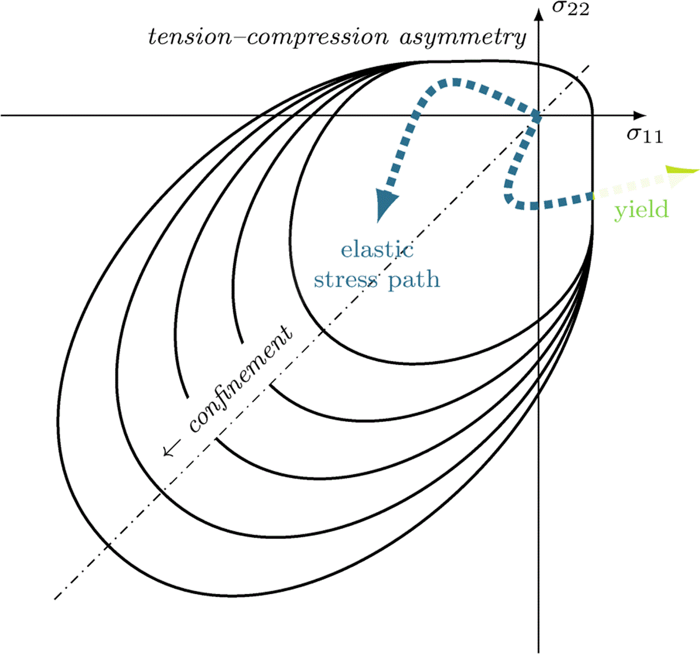
Figure 1. Schematics of a bi-axial failure surface expected for concrete with different levels of confinement.
Representation inspired from Torrenti et al.13
The main method followed in this study consists in
• postulating a linear thermoelastic regime (which overestimates stresses),
• then using a stress-based yield criterion to assess its validity in the considered applications.
In addition, the objective is to provide orders of magnitudes of mechanical states in ARC and to seek generalizable results in thermoelastic bi-materials.
To do so, reference materials are chosen and calibrated in section 2. Analytical and general results are sought in section 3 where yield functions are also introduced. The notion of yield distance is then clarified and a corresponding quantifier is constructed. Numerical cases make use of the identified conditions and the tools developed in section 4. Two case studies are investigated there, including a thermal stress estimation for general aluminium inclusions in concrete (expressed in stress per degree Celsius), as well as a mechanical criticality estimation during the curing of a composite beam.
2. Materials
In this section, we examine realistic orders of magnitude for the thermal and elastic parameters and the conditions under which they remain valid. The transient design situation (Eurocode 0) includes the curing of concrete which brings an important variation to its characteristics. In contrast, the reinforcement materials are already stabilized during the considered phase and are therefore treated as having constant behavior.
2.1. Aluminium
The present case study focuses on a conventional extrudable aluminium. It is chosen as Al–6082 in T6 condition and described by the product documentation of Hydro14. The limit stress is taken as the maximum failure stress in the provided low–cycle fatigue tests, that is 75 MPa which corresponds to over ten thousands cycles at room temperature with a load ratio of one half. The documentation provides the Young modulus
=70 GPa and the shear modulus
=26 MPa from which the Poisson ratio is deducted as
.
2.2. Concrete
The lightweight concrete (LWC) developed within the Made4Wind research project15 is classified as LWC45, with a characteristic compressive strength at 28 days (
) of 45 MPa. The Model Code16 (MC) was followed to determine the associated mechanical properties. According to Equation (14.6–2, MC), the average compressive strength is obtained by adding 8 MPa to the characteristic value, resulting in
53 MPa. Following Equation (14.6–3, MC), the characteristic tensile strength of LWC45 is determined for an oven-dry density of 1900 kg/m3.
• the mean tensile strength
4.05 MPa;
• the LWC strength reduction factor
0.92;
• the mean tensile strength for LWC
3.72 MPa;
• the characteristic tensile strength for LWC
= 0.7
2.60 MPa.
Regarding the modulus of elasticity, for normal-weight concrete made with natural sand and gravel, it can be estimated based on the specified characteristic strength using:
• the tangent elastic modulus at 28 days
26240 MPa;
• the initial modulus of elasticity
21.5
103 MPa;
• the coefficient
0.70 accounting for the aggregate type influence on stiffness;
• the stiffness reduction factor for LWC
0.75;
• the tangent elastic modulus for LWC at 28 days
19571 MPa.
According to the Model Code, for the design of structural members—particularly considering the influence of crack formation at the ultimate limit state (ULS), a Poisson’s ratio of
provides sufficient accuracy. Furthermore, for lightweight aggregate concrete, the coefficient of thermal expansion can be taken as
8
10−6 K−1.
The heat generated during concrete curing can impose the most restrictive design conditions in terms of maximum temperature and thermal gradients. Additionally, it is crucial to account for the precise mechanical properties of concrete at early ages, as cracking may occur due to incompatibility strains—for instance, in the case under study, where aluminum bars deform differently from concrete. To account for concrete strength development, the Model Code is once again referenced. Typically, the reference time is taken as 28 days, and the coefficient
depends on the concrete’s strength development class. For lightweight concrete, this coefficient depends on the aggregate strength, taking values of 0.05 for high-strength aggregates and 0.25 for low-strength aggregates.
(1)
The tensile strength is directly related to the compressive strength, developing over time at the same rate.
Regarding the time-dependent development of the modulus of elasticity, the coefficient
is directly related to
:
(2)
A semi-adiabatic experimental test (Heat-Box, similar to semi-adiabatic calorimetry EN 196–9:201017 and ASTM C1753–24 was conducted. This method is used to evaluate the heat evolution of concrete during early-age hydration by monitoring the temperature (by an embedded thermocouple) development of a fresh concrete specimen (about five liters) placed in a highly insulated container. By minimizing heat exchange with the surroundings, this approach enables the estimation of both the rate and cumulative heat of hydration under conditions that closely resemble real structural applications than isothermal calorimetry. The resulting temperature–time data are converted into heat release through an energy balance that accounts for the thermal capacity of the specimen and any heat losses.18 The measured data also provide essential input for numerical thermal models used to predict temperature development and assess early-age thermal cracking risk in concrete structures Results obtained for the test are presented in
Figure 2, showing a red curve reflecting that the maximum temperature for the LWC45 is reached at 17.5 hours. The same figure also displays three
curves. The dark blue and red curves represent the values provided by the Model Code, which depend on the aggregate strength, showing significant variability—from 0.27 for low-strength aggregates to 0.77 for high-strength aggregates. Given the aggregates used in this study, an intermediate value closer to the high-strength case was considered (
=0.1). These curves could be experimentally refined in future stages to enhance the accuracy of the analysis.
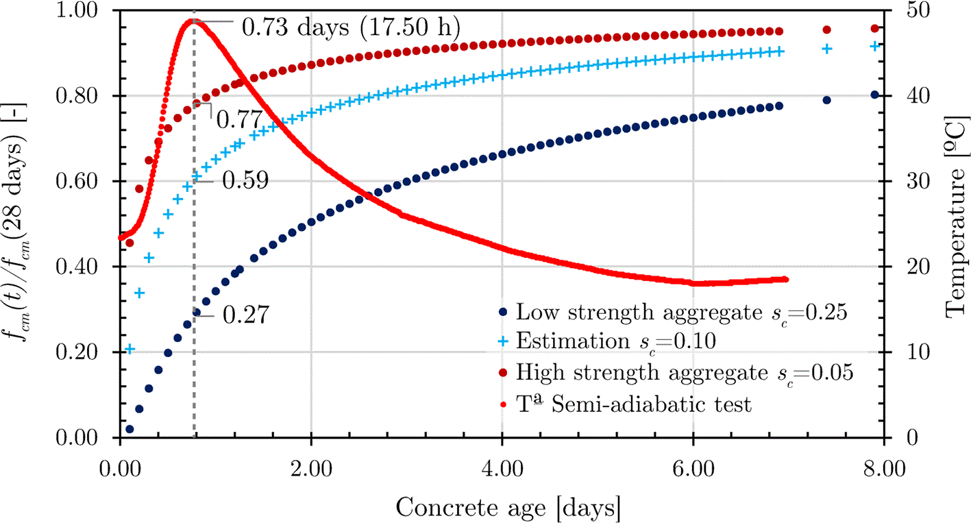
Figure 2. Concrete strength (computed analytically) and temperature development (measured experimentally) in semi-adiabatic conditions.
2.3. Steel
Steel is further employed as reference material (see Fig. 5). The steel values reported in
Table 1 refer to a conventional construction steel (S235).
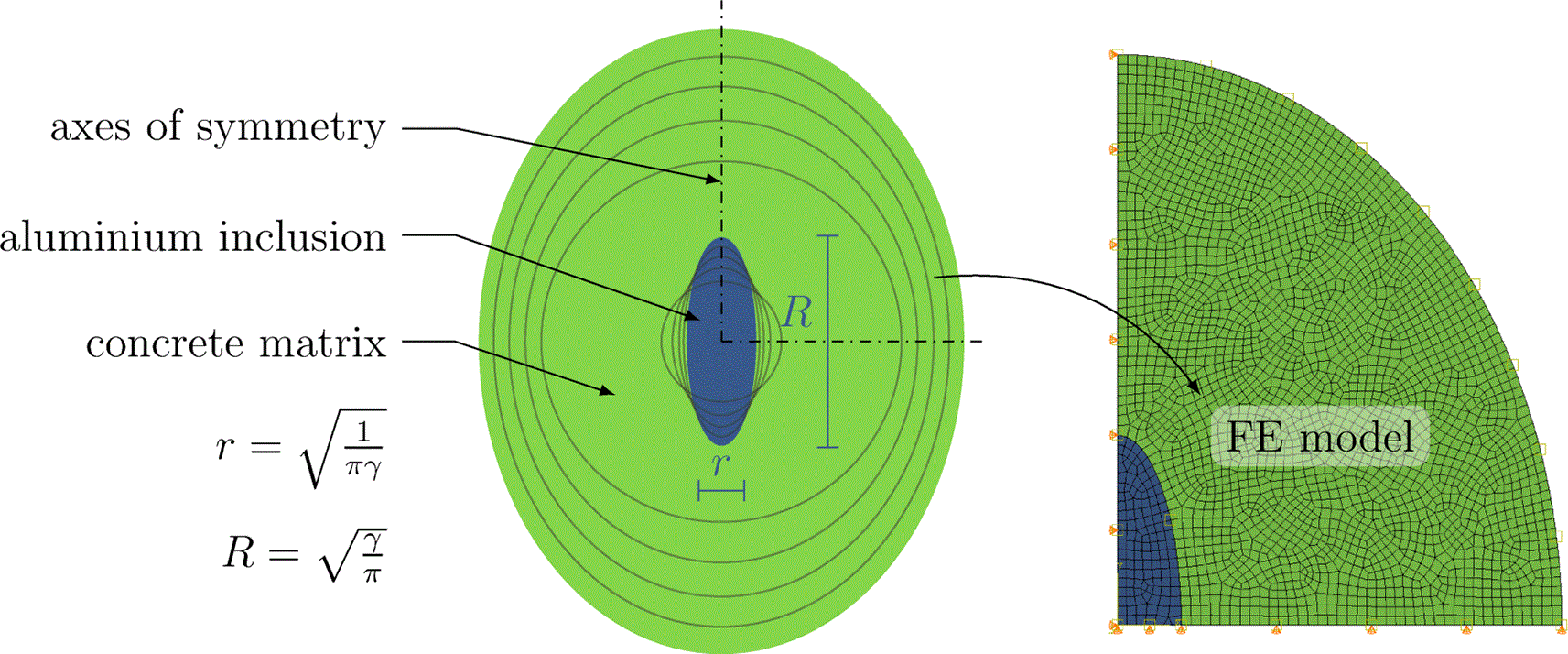
Figure 3. Ellipsoidal inclusions of constant unit surface areas and varying aspect ratio, and corresponding finite element mesh for an aspect ratio of 3.
The coating thickness is constant and equal to twice the largest radius.
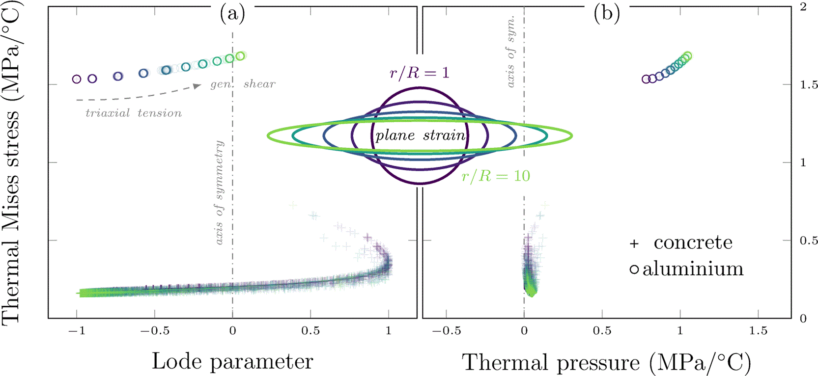
Figure 4. Ellipsoidal aluminium inclusion of varying aspect ratio and cross-sectional area.
Concrete matrix with free boundary conditions in plane strains.
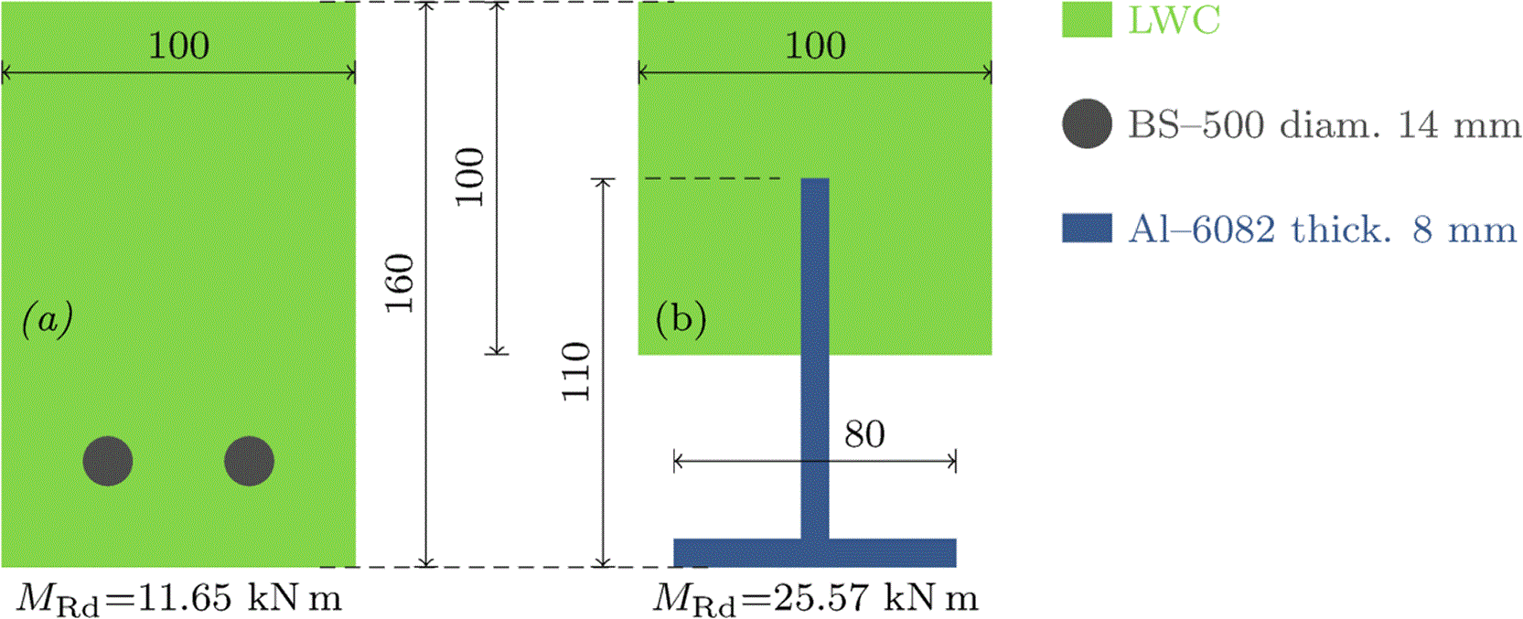
Figure 5. Conventional steel-reinforced beam chosen for reference (a), and corresponding aluminium-reinforced composite beam (b) with equal outer dimensions.
The steel surface area is
in (a) and the aluminium surface area is
in (b). Dimensions are given in mm.
Table 1. Thermo–elastic parameters for the reference materials.
The limit stress refers to a characteristic value justified under section 2. The concrete anisotropy is described by distinguishing the higher compressive strength form the lower tensile one:
and
. Metal limit stresses are taken as the conventional elastic limit measured measured at a tensile strain of 0.02, denoted
.
| Material | Young modulus | Poisson ratio | Limit stress | Thermal expansion coefficient | Thermal conductivity |
|---|
|
(GPa) |
(−) |
(MPa) |
(
) |
(
) |
| aluminium 6082–T614 | 70 | 0.346 | 260 (
) |
| 172 |
| concrete (LWC45) | 19.57 | 0.2 | 2.60 (
) to 45 (
) |
| n/a |
| steel (S235) | 210 | 0.3 | 235 (
) | n/a | n/a |
3. Analytical studies
3.1. General settings
We consider a linear thermo-elastic continuum, with quasi-static conditions and the absence of body forces. The domain geometry is arbitrary but the boundary conditions considered below are either free (nil surface tractions) or clamped (nil displacement).
Let a body occupies a configuration
subjected to small strains. The boundary of the domain is denoted
with its outer normal unit direction
. The domain is composed of several materials separated by interfaces that union is denoted
. The difference between the values of a field
on each side of the interface is called jump and denoted with the double square brackets
. The Frobenius norm of a symmetric tensor
is the scalar
computed as
or with Einstein’s notation
.
The kinematics of the body are described globally by the displacement field
, and locally by the (linearized Green–Lagrange) strain field
which is decomposed into a volumetric part
with
and deviatoric part
. They are connected by the compatibility equations
. Finally the stress is derived from the linear thermo-elastic constitutive model:
(3)
where
denotes the temperature field. The mechanical problem can be stated as follows.
Problem 1 (quasi-static, linear, isotropic, multi-phase thermo-elasticity). Given a temperature load
, find
• the displacement field
,
• the strain field
,
• the stress field
,
such that
(4)
(5)
(6)
The boundary conditions are written
(7)
(8)
Since several materials are considered, the interface conditions are expressed as
(9)
(10)
3.2. Free edges case
We take the case of a body subjected to no body forces and only free boundary conditions.
(11)
We seek trivial solutions
everywhere, letting both materials freely expand. Here the given boundary conditions and momentum balance equations (6) and (10) are immediately verified. The constitutive model (5) then yields
(12)
A simple way to cancel deviatoric strains is to find a potential
such that
which yields
(13)
The problem can be restated as:
, given a temperature load
, find
such that
(14)
For homogeneous temperature distributions, this is verified for any isotropic function of the form
(15)
which describes an isotropic expansion centered in
. Finally, the interface continuity condition imposes that the same potential is used which enforces a condition on the thermal expansion coefficient:
(16)
Result 1.
Under a uniform thermal load with free boundary conditions, the stress is nil and the strains continuous when thermal expansion coefficients are uniform.
3.3. Confined case
We now consider the case of perfect confinement where the entirety of the domain boundary is held in place and no forces are imposed
(17)
We raise the question of the existence of trivial solutions where temperature can vary within the body while not causing any deformation. That is, we postulate
and investigate the consequences on the other variables and parameters to be held true.
No deformations implies no strains and purely thermal stress, hence
(18)
(19)
The bulk equilibrium becomes
(20)
which imposed a homogeneous temperature over the domain. Finally the interface conditions are trivially verified in displacements (nil everywhere) and require that the stress jump
(21)
which is verified if, and only if,
(22)
Result 2.
Under a uniform thermal load with clamped boundary conditions, the strains are nil and the stress continuous when the “thermal stiffness” coefficients are uniform.
3.4. Yield functions
The notion of yield here describes the end of a purely elastic regime, when part of the strain energy gets exchanged irreversibly. It can be materialized by the onset of plasticity, a loss of stiffness (continuum damage) or the nucleation of cracks. Its mathematical description often relies on a yield function
(23)
where function
is named equivalent stress, and
the yield stress. The yield function
is at least expected to be semiconvex. The failure criterion is then represented by the inequality:
(24)
3.4.1. Aluminium yield
Alloy Al 6082–T6 can be represented by isotropic pressure independent equivalent stresses of the von Mises type:
(25)
where
is the Frobenius norm and the deviatoric part
In tension, yield is reached at
which lets us identify
(26)
3.4.2. Concrete yield
Concrete LWC45 and granular materials require to take into account the strengthening effect brought by confinement as illustrated in 1. To do, models such as Mohr–Coulomb,19 Drucker–Prager20 or Spitzig–Richmond (Mises)21 take into account a dependence to pressure (the stresses’s trace). Other popular alternative include Ottosen22 or William–Warnke23 yield functions that include a Lode angle dependency to distinguish generalized tension and compression in the deviatoric behavior. In this study and with the availability of two resistance values (in tension and compression), we choose the Drucker–Prager form
(27)
characterized by a linear dependency with pressure.
Using table 1, the limit states are reached in tension for
and in compression for
. The parameters identification returns:
(28)
The time dependency of these parameters are controlled by
.
3.4.3. Yield distance
This study requires a measure that expresses the criticality of given stress state, that is an indication of distance (in the sense of the Frobenius norm
) between a stress tensor and the concrete yield surface. The shortest possible distance for a given stress
, using the decomposition
and
; then reads
(29)
This is a signed distance which returns a negative value inside the yield surface, and a positive value beyond yield. The magnitude of
has the unit of the stress and corresponds to the smallest added load needed to bring the considered material point to yield, hence it gives a concrete information on the criticality of a given stress. Geometrically, it corresponds to the length of a segment drawn between the stress and its orthogonal projection on the Drucker–Prager cone. The developments of this results and connected minimization problem are detailed in Appendix A.24
4. Numerical cases
This section focuses on identifying and investigating first order challenges in aluminium–reinforced concrete. It is widely emphasized in the literature that the first detrimental factors to be accounted for are
But depending on the combinations of material behavior, case load and the parts geometry, residual stresses can range anywhere from negligible to significant. A similar argument is valid concerning the assumptions of perfect bonding and thermo–elastic linearity: they are acceptable under small stresses, and less and less valid as the mechanical states is brought closer to the yield surface. A quantitative measure is given in section 3.4.3 and used further, but the first step proposed below is to establish both a quantitative and a qualitative estimate of the mechanical state brought by thermal loads.
4.1. Ellipsoidal inclusions
This case study aims to evaluate the stress states directions and intensities that can be expected for geometries typically encountered in reinforced concrete, that is aluminum inclusions in concrete matrices.
The parametric geometries are described in
Figure 3. It presents an ellipsoidal inclusion with an aspect ratio of 3, and a concrete coating of constant thickness. The study uses 10 tests with aspects ratios ranging from 1 to 10. The maximal and minimal radii of the inclusion are chosen such that the surface area of the aluminum is always equal to
. Note that the stress results are scale–independent, hence the arbitrary area. The thickness of concrete coating is homogeneous and equal to twice the largest inclusion radius: this ratio is chosen after a convergence study in order for the stress norm to be negligible near free edges.
The finite element (FE) model is built using Abaqus interfaced with ISight. The mechanical boundary conditions are free edges and plane strains, and the model exploits the two axial symmetries of the section to use a quarter of it for the simulations. The mesh uses fully integrated quadrangles of imposed size 0.05 with deviation factor 0.1. These parameters were picked after a convergence study for the largest aspect ratio of 10. Finally, similar studies under modified symmetries are presented under Appendix B.24
The thermal load is an imposed homogeneously distributed temperature increment of
. Since the entirety of the problem is linear, all solutions (displacements, strains and stresses) are proportional to the temperature increment, which means they can be expressed per unit of temperature and fosters the range of conclusions—as long as linear assumptions remain meaningful. As shown below, this also mean that a negative temperature step will return tension where compression would be caused by a positive step, and conversely.
Figure 4 summarizes the results of the parametric study. In order to give a comprehensive representation of stress states, the two graphs feature three axes to uniquely represent isotropic stress states.
• The Lode parameter represents the tensorial direction in the deviatoric plane: −1 corresponds to generalized compression, 0 to generalized shear and +1 to generalized tension.
• The thermal Mises stress gives the magnitude of the stress tensor projected onto the deviatoric plane, per unit of temperature.
• The thermal pressure corresponds to (a third of
) the trace of the stress tensor, and geometrically gives the altitude of the vector perpendicular to the deviatoric plane per unit of temperature.
Each marker on the graph represents the stress state obtained at the integration point of one of the finite elements of the model after the load. The markers are circles for aluminium (o), and crosses for concrete (+). Marker colors (from dark blue, 1, to light yellow, 10) maps to the aspect ratio of the corresponding simulation, which is also represented in the central figure. They are plotted with a high transparency such that the accumulation of points accentuates their color, and gives an intuition of population density. Aluminium area (and number of elements) is held constant but the concrete area (and number of elements) increases with increasing aspect ratio because of an increasing coating thickness.
The vertical dashed lines represent axes of symmetry: the graphs would be mirrored around them if the temperature increment had been negative. This is important to emphasize since it means that the Lode angle and pressure results are just as likely to be inverted.
The yield behavior of aluminium being largely isotropic in the deviatoric plane, and presenting negligible pressure sensitivity,21 the variation of Lode parameter and slight increase in thermal pressure brought by shape change is not expected to bring any significant impact over the reinforcements. However, the order of magnitude of Mises stress goes beyond
and increases by up to 15% as the profile’s curvature increases. With realistic thermal loads ranging to dozens of degrees, such a stress concentration magnitude would represent 20 to 30 MPa hence should be taken into account in the safety margin of designs.
The concrete stress states span over the entire deviatoric plane, although increasing aspect ratios under positive (resp. negative) temperature increment focuses them towards triaxial tension (resp. compression) and decreases the deviators’ magnitudes. They remain smaller than that of aluminum by a factor up to 3 to 4, which also corresponds to the difference of scale between the Young moduli of aluminium and concrete in this plane strain scenario. It is shown in Appendix B24 that the same is not found in the plane stress case, which displays lower stresses of globally similar magnitudes in the two material phases.
If moderate, a negative pressure can increase the concrete resistance through an effect of confinement as described by the choice of Drucker–Prager yield function in the previous section. But positive pressure corresponds to tensile states that meet a much lower resistance in concrete. Considering the axis of symmetry, any significant pressure in
Figure 4 should be considered detrimental regardless of its sign. The order of magnitude here is
, which would represent 2 MPa for an increment of
for is low enough to maintain the relevance of the assumption of linearity, but also high enough to require to be taken into account in a design context.
4.2. Composite beam
As emphasized in section 2, the earliest life of ARC needs to be studied since, during the first hours of curing, the largest temperature steps are observed while the concrete resistance and stiffness continue to increase. Therefore a competition is expected between the stresses increasing with stiffness, and the resistance that also grows during curing. The resulting behavior can hardly be predicted without the analysis proposed below. It relies on the materials identified in section 2 as well as the yield distance defined section 3.4.3 which measures the criticality of a given stress state given an evolving yield surface.
This case study focuses on realistic orders of magnitudes expected during the curing of an aluminium-reinforced concrete beam. To do so, the modified clothoidal composite dowel (MCL)25 is selected. An I–beam is extruded and cut into two identical T–beams that profile is optimized to be obtained with the least number of cuts possible, to favor adherence and to minimize fatigue.
Figure 5 presents the reference geometry used in the numerical case study. The aluminium–concrete composite section leverages the mechanical contribution of an extruded Al-6082 T-profile placed at the tensile zone, resulting in a 119% increase in bending resistance compared with a conventional steel-reinforced section of identical outer dimensions. This comparison is included solely to contextualize the case-study geometry.
The longitudinal profile and the discretized geometry is detailed in
Figure 6. The computation is performed using commercial software Abaqus26 and prescribes an evolving homogeneous temperature field that amplitude is computed in 2 and shown in
Figure 2. While aluminium parameters are approximated as constant, concrete stiffness and yield parameters are evolving function of
defined in
Equation 1.
(30)
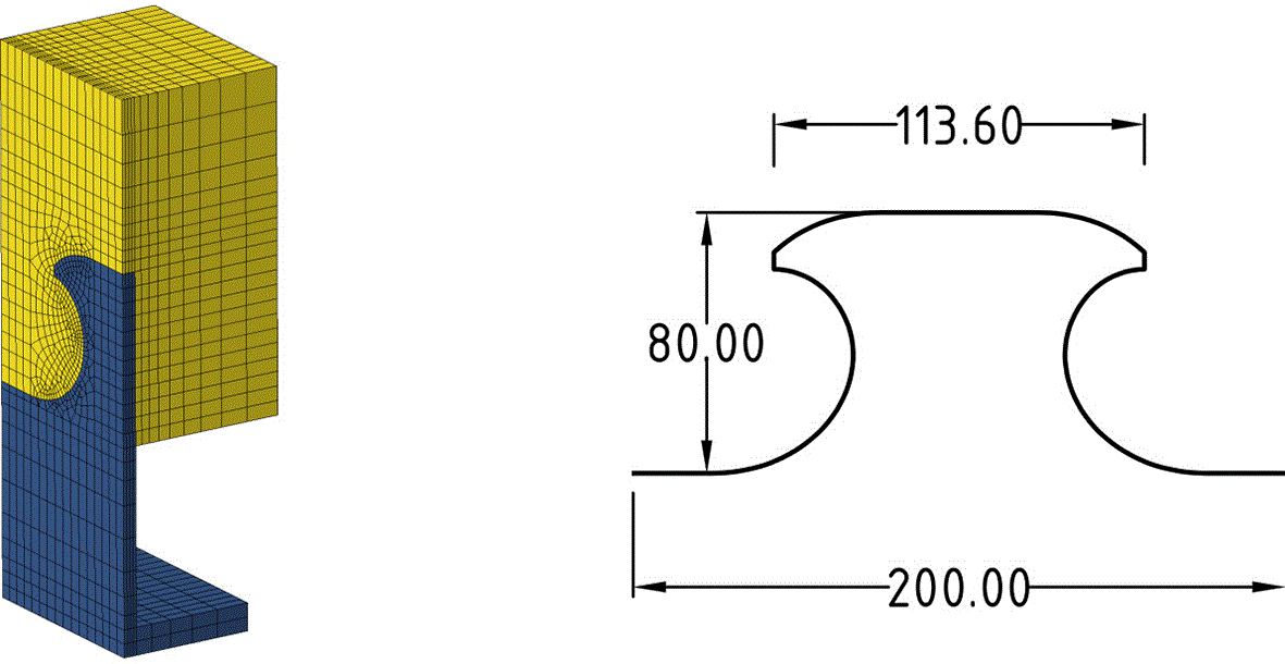
Figure 6. Dimensions and finite element discretization of the cast MCL.25
The Abaqus model includes 10555 nodes, 8938 linear hexahedral elements (C3D8R) and 312 linear wedge elements (C3D6). It exploits the symmetry of the geometry and that of the plane strain conditions to represent a beam of arbitrary length.
The beam section is held in plane strain boundary conditions which is both realistic for and extruded element, and conservative as preventing strains maximizes stresses.
Figure 7 indicates the cumulative histogram of the yield distance during the concrete curing. To obtain the plot, the yield distance is computed at each time increment and each finite element centroid, and its value weighed by the initial volume of the corresponding element (proportional to its mass). Only the concrete elements are kept for the computation. The x–axis represents curing time, and the y–axis the yield distance, while the surface color indicates the bin height, which givens the proportion of concrete the yield distance it less than the corresponding value. When the surface is brightest (i.e. the bin height is 1), then every concrete particle is further from yield. Conversely, the darkest areas report that all concrete particles are closer to yield than the corresponding value. In between the two zones, a sharp front shows where most of the particles lie.
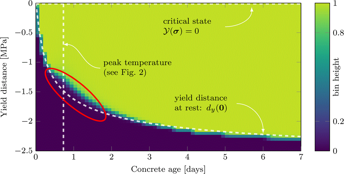
Figure 7. Cumulative histogram of the yield distance in concrete during setting of the composite beam design.
The data comes from concrete elements centroids of the thermo-elastic simulations of the model from Fig. 6, and is weighed by the element’s initial volume.
To help with analysis, three annotated lines are added. The vertical one reports the maximum imposed temperature. The top horizontal line emphasizes the zero-distance axis, which corresponds to yield. The annotated curve indicate what yield distance is measured for any concrete particle that suffers no stress. It serves as reference to compare with the evolution of the histogram’s front, and emphasizes how the vast majority of the concrete region keeps small to negligible stress states throughout the curing process. The histogram’s front mainly detaches from the reference curve around the peak temperature, but added stresses remain marginal when compared to the expansion of the yield surface. The competition between increasing stiffness (combined with fast evolving temperature) and increase material resistance during curing does not bear detrimental consequences in the considered case.
5. Conclusions
This paper provides basis for the thermo-mechanical study of ARC following recent chemical improvement of aluminium–concrete interfaces. It develops and makes uses of the following methods.
• The exploitation of linear assumption to provide first order simple estimates of thermal stresses.
• The yield distance as a design tool to track the criticality of stress states and the relevance of the aforementioned assumptions.
The main results include the following.
• Analytical theorems on the continuity conditions of strain–stress fields in bi-materials. While unfit for the materials chosen in this study, these results can help the understanding and choice of composites beyond the ARC context.
• Thermal stresses in aluminium–concrete inclusions. The computed orders of magnitudes indicate the possibility of compatible ARC designs, but emphasize the necessity of a systematic thermo-mechanical analysis.
• Yield distance estimates in curing, with numerical evidence that stresses can remain acceptable in conservative conditions while casting a composite beam.
The methods above ought to be used in a pre-design context, and the output thermal stresses could be included either as initial condition for structural integrity checks, or be converted into additional safety factors. To dive deeper into ARC design complexity, the next steps of this research shall include cohesion defects at the concrete–aluminium interface and move towards non-linear regimes.
Ethics and consent
Ethical approval and consent were not required.
Acknowledgements
Generative AI: GPT-4o was used via the Microsoft Copilot interface for language improvement in the Abstract and Introduction.
References
- 1.
Glosser D, Choudhary A, Isgor OB, et al.:
Investigation of reactivity of fly ash and its effect on mixture properties.
ACI Mater. J.
2019; 116(4): 193–200. Publisher Full Text
- 2.
Kleinau KF:
Development of environment-friendly concrete constructions by use of aluminium reinforcement.
NTNU;
2022. Master’s thesis.
- 3.
Fagermo MM:
The use of aluminium in sustainableconcrete structures.
NTNU;
2020. Master’s thesis.
- 4.
Freedman S:
Corrosion of nonferrous metals in contact with concrete.
Modern Concrete.
1970; 36.
- 5.
Grubb JA, Limaye HS, Kakade AM, Testing pH of concrete. (
2007).
- 6.
Khan MS, Trejo D, Guide to design and construction practices to mitigate corrosion of reinforcement in concrete structures, aCI 222.3R-11. (
2011).
- 7.
Szumigala M, Polus Å:
Applications of aluminium and concrete composite structures.
Procedia Eng.
2015; 108: 544–549. Publisher Full Text
- 8.
Chybiński M, Polus Å, Szumigala M:
Aluminium members in composite structures, a review.
Arch. Civ. Eng.
2022; 253–274. Publisher Full Text
- 9.
Zhou F, Young B:
Tests of concrete-filled aluminum stub columns.
Thin-Walled Struct.
2008; 46(6): 573–583. Publisher Full Text
- 10.
Channa IA, Saand A:
Mechanical behavior of concrete reinforced with waste aluminium strips.
Civil Engineering Journal.
2021; 7(7): 1169–1182. Publisher Full Text
- 11.
Justnes H:
Durable aluminium reinforced environmentally-friendly concrete construction–dare2c.2017.
- 12.
Wang YP, Fagermo M, Furu T, et al.:
Compatibility of different aluminium with a new environmental-friendly concrete.
7th Non-Traditional Cement and Concrete, Vol. 145 of NTCC2023.
Trans Tech Publications Ltd;
2024; pp. 97–104. Publisher Full Text
- 13.
Torrenti J-M, Reynouard J-M, Pijaudier-Cabot G:
Mechanical Behavior of Concrete.
London:
Wiley;
2013. published Online: 8 MAR 2013. Publisher Full Text
- 14.
Hydro, Alloy EN AW–6082 [AlSi1MgMn], Technical datasheet.Jan. 2019.
- 15.
Made4Wind. horizon europe research and innovation funding programme under grant agreement number 101136096.
http
- 16.
fib:
fib Model Code for Concrete Structures 2010, Vol. 1 of Bulletin.
Lausanne:
Wiley;
2013. Publisher Full Text
- 17.
Methods of testing cement. part 9: Heat of hydration; semi-adiabatic method, European Committee for standardization.2003.
- 18.
Schindler AK, Folliard KJ:
Heat of hydration models for cementitious materials.
ACI Mater. J.
2005; 102(1): 24. Publisher Full Text
- 19.
Coulomb CA:
Essai sur une application des règles de maximis et minimis à quelques problèmes de statique, relatifs à l’architecture, Mémories de Mathématique et de Physique présentés à l’cadémie Royale des Sciences.1776. Publisher Full Text
- 20.
Drucker DC, Prager W:
Soil mechanics and plastic analysis or limit design.
Q. Appl. Math.
1952; 10(2): 157–165. Publisher Full Text
- 21.
Spitzig WA, Richmond O:
The effect of pressure on the flow stress of metals.
Acta Metall.
1984; 32(3): 457–463. Publisher Full Text
- 22.
Ottosen NS:
A failure criterion for concrete.
J .Eng. Mech. Div.
1977; 103(4): 527–535. Publisher Full Text
- 23.
William KJ, Warnke EP:
Constitutive model for the triaxial behavior of concrete.
International Assoc. for Bridge and Structural Engineering;
1975.
Reference Source
- 24.
Reyne B, Ruiz Maestre R, Delhaye V, et al.:
Thermomechanical viability of aluminium-reinforced concrete: simulation data.Jul. 2026. Publisher Full Text
- 25.
Lorenc W, Kozuch M:
Development of the modified clothoidal (mcl) shape of composite dowels against the background of fatigue and technological issues.
Studia Geotechnica et Mechanica.
2024; 46(2): 91–110. Publisher Full Text
- 26.
Abaqus:
Abaqus user subroutines reference guide, Dassault Systèmes, 2014.2014.
Reference Source







