1. Introduction
Lithium-ion batteries are widely deployed in a broad range of applications, including portable electronics, electric mobility, renewable energy storage, and grid-scale systems.1 As their adoption continues to expand, ensuring their efficient use throughout their lifetime has become a critical challenge. To make the most of this resource, extending battery life beyond its first use has emerged as a key strategy within the framework of circular battery value chains.2 Ensuring the safety, reliability, and predictable performance of retired batteries enables the repurposing and reuse of these batteries in further applications, improving battery profitability and reducing at the same time the environmental impact of these batteries.
In this context, battery sorting into recycling or further use is essential, as batteries with similar apparent performances may exhibit fundamentally different internal degradation states that could limit reuse capabilities. The UL1974 standard3 proposes testing and evaluation procedures for battery repurposing and remanufacturing, focusing on the electrical performance, safety screening, and basic health indicators. Although practical and standardized, these tests provide limited insight into the underlying degradation mechanisms. Similarly, existing academic and industrial sorting approaches often rely on readily available indicators, such as BMS-reported state-of-health (SOH), which lack diagnostic depth.4,5 More advanced techniques, including electrochemical diagnostics, data-driven methods, and imaging-based approaches,6,7,8 can improve sorting accuracy but typically require intrusive measurements or specialized equipment, limiting scalability.
A key limitation of current second-life assessment strategies is that the SOH alone is insufficient to characterize battery degradation. In particular, the loss of lithium inventory (LLI) and loss of active material (LAM) affect batteries differently in terms of their efficiency, power capability, safety, and long-term reliability.9,10 However, standard second-life testing procedures, including UL1974, do not provide sufficient electrochemical information to distinguish between the degradation modes. Non-destructive techniques, such as incremental capacity analysis and differential voltage analysis, can extract degradation-related information, linking peak shifts to LLI and peak spacing changes to LAM,11,12 but traditional implementations are time-consuming and unsuitable for fast, large-scale end-of-life sorting.
To address these challenges, this work proposes a lightweight diagnostic and classification framework that combines electrochemical testing with machine learning to quantify the dominant degradation modes in end-of-life lithium-ion batteries. By leveraging full incremental capacity profiles and artificially generated degradation scenarios, the proposed approach provides scalable mechanism-aware insights. The provided insight regarding the aging mechanisms (LLI and LAM) allows the identification of damage at the electrode level, enabling more reliable sorting and classification than the traditional ones.
This paper is organized as follows: Section 2 describes the methodology for creating an LLI and LAM quantification model; Section 3 outlines the LLI and LAM degradation mechanisms; Section 4 describes the generation of LLI- and LAM-induced synthetic data as well as how the half-cell level data were obtained for this purpose; Section 5 details the characteristics of the selected machine learning model as well as the methodology followed up to train and verify the performance of the model; Section 6 describes two second life sorting use cases and the developed LLI and LAM quantification models; finally, Sections 7, 8, and 9 present the results, followed by the discussion and the conclusions of the paper.
2. LLI and LAM quantification model
The observable decrease in battery performance is due to an increase in the resistance and a decrease in the dischargeable capacity.13 The cause of this performance decrease is related to the intrinsic characteristics of the cell, which are mainly related to the number of lithium ions available inside the cell (also called the lithium inventory) and the available active material that can react with the lithium ions of each electrode.
Batteries that come from their first end of life, to be used afterwards in a second life application, are often sorted based on the measured pure ohmic resistance response at a certain state of charge and the measured dischargeable capacity. Nonetheless, the actual causes of the increase in the resistance and decrease in the discharge capacity cannot be measured using non-invasive methods. However, it was not possible to detect the limiting components. Consequently, in this study, a model that can provide information about the LLI and LAM of each electrode, based on measurable elements, was developed. This model provides more insight into the battery SOH by identifying the limiting element.
• A predominant LAMne indicates that the anode limits the SoH (cathode material has a performance decrease).
• A predominant LAMpe indicates that the cathode limits the SoH (anode material exhibits a performance decrease).
• The predominant LLI indicates homogeneous degradation at the cell level (lithium ions have been consumed).
The methodology to develop this model is described in
Figure 1.
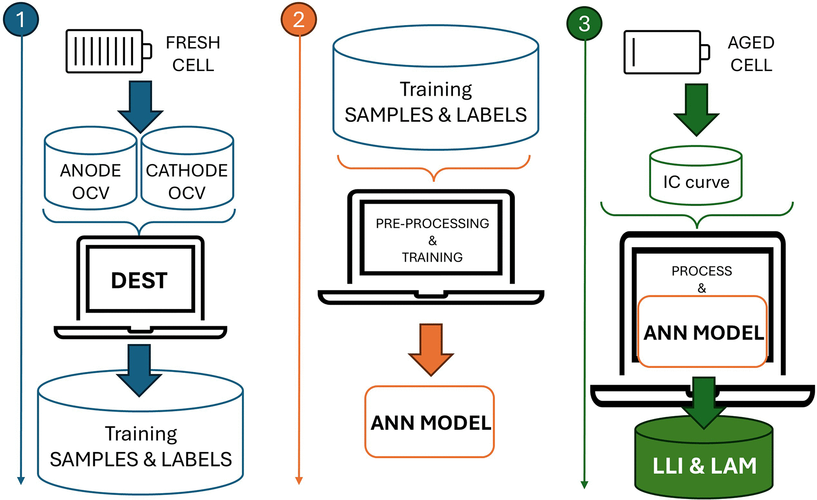
Figure 1. Methodology on how to develop and apply a LLI and LAM quantification model.
First, the samples and labels used to train the machine learning model were generated. The incremental capacity (IC) curves are artificially generated at a range of LLI and LAM values using the DEST tool,14 which uses half-cell level data of the cells that must be sorted in a fresh state.
Second, a machine-learning model was developed. The previously artificially generated IC curves along with the generic aging modes (LLI LAMne and LAMpe) were pre-processed and then used to train and verify the model.
Finally, the IC curves of the batteries that come from the first end of life were obtained from experimental testing, processed to match the input format of the developed model, and passed to the model to obtain the LLI and LAM of each electrode, allowing a deeper insight into the SOH of the batteries by identifying the limiting cell component (anode, cathode, or available lithium ions).
3. Degradation parameters
Battery degradation in lithium-ion cells is commonly characterized by two dominant mechanisms: Loss of Lithium Inventory (LLI) and Loss of Active Material (LAM). These degradation modes alter the electrochemical balance of the cell and directly affect the shape and evolution of Incremental Capacity (IC) curves. To reproduce these effects, degradation was mathematically incorporated into the electrode stoichiometry and capacity scaling parameters using the formulations proposed in,14 which are presented in detail in Section 4.
3.1 Loss of lithium inventory (LLI)
LLI represents the consumption of cyclable lithium by parasitic side reactions, such as the growth of a Solid Electrolyte Interphase (SEI).
• Mathematical Representation: In equations, the LLI is modeled by adjusting the slippage between the electrode stoichiometry ranges.
• Physical Interpretation: As lithium is consumed, the electrodes become "desynchronized." For instance, the negative electrode may no longer reach a fully lithiated state because the system-wide lithium inventory is insufficient to fill available host sites.
• IC Curve Effect: This physical shift manifests as a horizontal translation of the IC peaks. As the "lithium window" shrinks, the peaks at the voltage extremes may disappear.
3.2 Loss of active material (LAM)
LAM refers to physical degradation of the electrode lattice, such as particle cracking, exfoliation, or loss of electrical contact.
• Mathematical Representation: LAM is modeled using scaling factors applied to the capacity of the individual electrodes.
• Physical Interpretation: This indicates a reduction in the number of available sites for lithium intercalation. Even if the Li inventory is high, there is no "room" for intercalation to occur in the damaged host structure.
• IC Curve Effect: Because less active material to undergo phase transitions at specific potentials, the IC peaks undergo vertical compression (squashing).
4. LLI and LAM induced data generation
The mathematical formulation for generating the LLI and LAM data is based on the principle of electrode superposition. The full-cell open-circuit voltage was derived from the difference between the equilibrium potentials of the positive and negative electrodes.
To ensure the validity of this model, the following physical assumptions are maintained:
• Thermodynamic Equilibrium: The electrodes were treated as independent thermodynamic systems. The full-cell voltage is the potential difference between these two half-cells in the zero-current state.
• Spatial Homogeneity: Degradation is assumed to occur uniformly across the electrode surface. This allowed us to use lumped parameters rather than spatially resolved 3D models.
• Linear Scalability: The capacity of each electrode is assumed to be directly proportional to the mass of the active material available for lithium intercalation.
Based on this formulation, synthetic degraded pseudo-open-circuit voltage (pseudo-OCV) curves were created using the mathematical framework proposed in14 to generate the dataset required for training the machine-learning model. The tool presented in14 DEST enables the simulation of both fresh and degraded full-cell pseudo-OCV curves based on the experimentally measured pseudo-open-circuit potential (pseudo-OCP) curves of the individual electrodes.
The pseudo-OCP and pseudo-OCV curves are expressed in the general form
, where
denotes the capacity,
is the corresponding voltage/potential, and
is a function describing the voltage as a function of capacity.
The synthetic fresh pseudo-OCV curve was constructed from the pseudo-OCP curves of the positive electrode (PE) and negative electrode (NE) using Equations (1) and (2), respectively:
(1)
(2)
and voltage is obtained through the
Equation (3):
(3)
where:
• Subscripts
and
refer to capacity and voltage, respectively.
•
accounts for dimensional differences between the individual electrodes and the assembled full cell.
•
is the scaling factor used to adjust the negative electrode capacity when necessary. In most cases,
.
•
represents the relative shift between the electrodes, typically associated with solid electrolyte interphase formation.
•
denotes the voltage shift induced by the internal resistance. According to the adopted sign convention, this term is negative during discharging and positive during charging, resulting in a rigid translation of the curve along the voltage axis.
First, a voltage window must be defined to obtain an experimental pseudo-open-circuit voltage (OCV) curve. The points corresponding to the minimum and maximum voltages were identified as the End of Discharge (EoD) and End of Charge (EoC), respectively. Accordingly, the simulated pseudo-OCV curves were defined within the same voltage limits. After construction, the simulated curve was fitted to the experimental data to estimate the parameters
,
,
, and
.
Degraded pseudo-OCV curves were generated by incorporating degradation mechanisms into the electrode capacity transformation, as shown in Equations (4) and (5) as follows:
(4)
(5)
and voltage is calculated through
Equation (6):
(6)
where
represents the voltage shift due to the internal resistance in the degraded cell, again acting as a translation along the voltage axis.
The subscripts “li” and “de” denote lithiated and delithiated states, respectively. The degradation parameters (LLI and LAM) were defined in the range [0, 1], where 1 corresponds to the maximum degradation level. As with the fresh cell, EoC and EoD must be identified for the degraded cell because the pseudo-OCV curve is defined only within these voltage limits. For a given fresh pseudo-OCV curve, different degraded configurations may produce equivalent degraded pseudo-OCV curves, if they share identical aggregated degradation metrics. These aggregated quantities are defined in Equations (7), (8), and (9):
(7)
(8)
(9)
Consequently, the tool generates degraded pseudo-OCV curves characterized by the global degradation indicators
,
, and
, without distinguishing between their specific lithiated and delithiated contributions.
A large synthetic dataset of pseudo-OCV curves was obtained through systematic variation of these degradation parameters. This dataset provides labeled degradation scenarios suitable for the supervised training of the machine learning model.
4.1 Half-cell data generation
The experimental potential vs. capacity profiles (pseudo-OCP curves) of the PE and NE used to generate synthetic pseudo-OCV curves for the experimental full-cell data were obtained by testing at C/20 current rates PE||Li metal and NE||Li metal coin cells. Electrode level coin cells are built by first retrieving the electrode material of Beginning of life (BOL) comercial cells that are opened in a controlled argon environment. The electrode-level material was then properly washed to eliminate possible electrolyte residues. Next, the active material of one of the sides is removed to have the collector visible, followed by drying to be cut into coin cell format pieces of one side electrode. Finally, the coin cells were assembled with the electrode material, separator, lithium, electrolyte, and housing.
5. ML model
The chosen machine learning model is a Multi-Layer Perceptron (MLP).
An MLP is a type of neural network with one or more hidden layers of neurons connected in a feedforward manner. It has at least three layers: the input layer, hidden layer, and output layer. The input layer determines the input format. The hidden layer processes information using nonlinear activation functions. This layer is responsible for identifying the patterns in the data. The output layer determines the output format and provides the model results.
The MLP was chosen because it has already shown accurate results when relating to IC curves and SOH in previous works in the literature,15,16 so it is expected to accurately relate LLI and LAM with these types of curves.
6. Use cases
Two use cases with two different types of lithium-ion batteries (lithium nickel manganese cobalt oxides or NMC and lithium iron phosphate battery or LFP) were studied to test and validate the proposed LLI and LAM quantification models for second-life sorting.
6.1 NMC
The NMC cells coming from the first end of life are cylindrical DMEGC cells, model INR 18650-29E (see datasheet main parameters in
Table 1).
Table 1. Main parameters of NMC cell.
| Name |
Value |
|---|
| Nominal capacity | 2.9 [Ah] |
| Discharge cut off voltage | 2.5 [V] |
| Charge cut off voltage | 4.2 [V] |
These cells have been used as auxiliary power supplies in light commercial vehicles for the first time. The sorted cells were reused in the residential energy storage.
6.2 LFP
The LFP cells coming from the first end of life are prismatic CALB cells, model L135F72 72A (see the datasheet main parameters in
Table 2).
Table 2. Main parameters of LFP cell.
| Name |
Value |
|---|
| Nominal capacity | 72 [Ah] |
| Discharge cut off voltage | 2.5 [V] |
| Charge cut off voltage | 3.65 [V] |
These cells have been used in off-road industrial mobility applications, specifically in industrial forklifts. The cells were used in European warehouses.
The sorted cells will be reused in a 52 KWh C&I ESS system for grid-scale storage demonstration.
7. Results
The proposed methodology has been applied to both use cases where the half-cell data at a fresh state are presented, the artificially generated IC curves are shown, the MLP model verification is presented, the experimental tests performed on the cells to be sorted are shown, and the results from applying the LLI and LAM quantification models are disclosed.
7.1 Half-cell data
An NMC cylindrical cell and an LFP prismatic cell (both BoL) were opened and disassembled to obtain electrodes for coin cell preparation.
The extracted electrodes were washed three times with dimethyl carbonate to remove any remaining electrolyte residue. Then, one of the electrode coating sides of the double-sided electrodes was removed using water as the solvent for NE and N-methyl pyrrolidone for PE.
After drying the electrode materials under reduced pressure at 120 °C for 16 h, the electrodes were punched into discs of 16.6 mm diameter and coin cells were assembled using a Whatman GF/D separator (diameter 18.2 mm) and 100 μL of 1M LiPF6 in ethylene carbonate: ethyl methyl carbonate 3:7 (w/w) as the electrolyte.
PEs and NEs retrieved from the NMC cylindrical 2.9 Ah cell exhibited an average areal capacity of 3.6 mAh cm2 and 4.5 mAh cm2, respectively (N/P balancing factor 1.25). Electrodes obtained from the prismatic LFP 72 Ah cell had an average areal capacity of 2.4 mAh cm2 (PE) and 2.6 mAh cm2 (NE) corresponding to an N/P balancing factor of 1.1.
All half-cell coin cells were tested at C/20 current rates (relative to the actual capacity of the coin cell) at 25 °C using a BaSyTec BST cycler to obtain the electrode pseudo-OCP curves, as shown in
Figure 2.
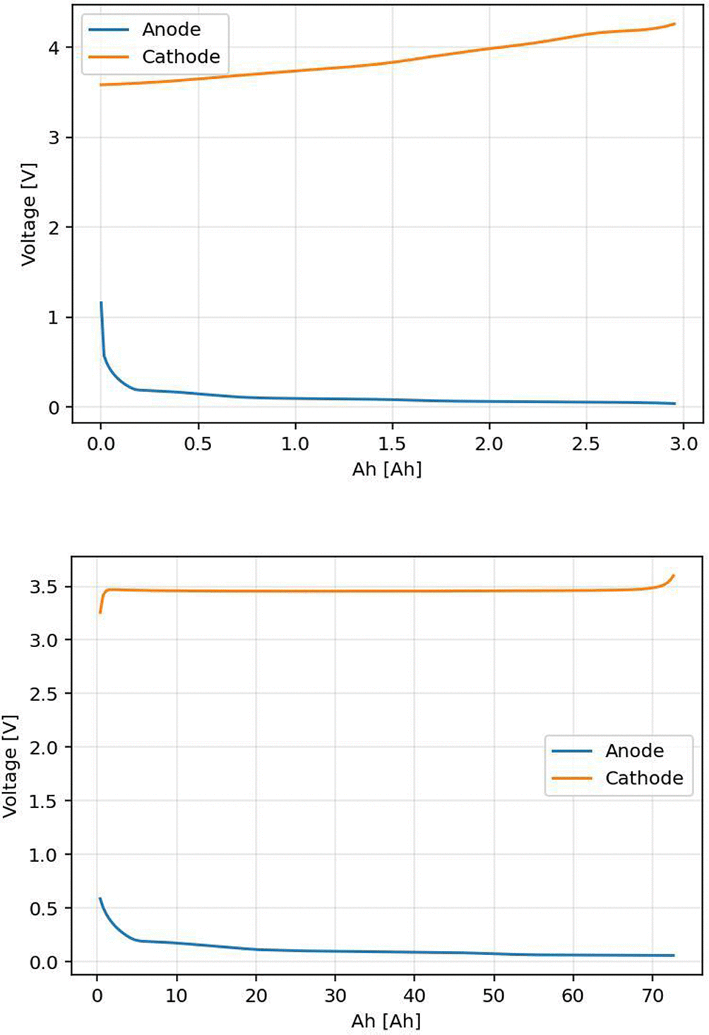
Figure 2. Pseudo-OCP curves of NMC (up) and LFP (down) electrodes.
OCP curves with extended voltage/potential operation windows were used to obtain a realistic representation of the synthetic pseudo-OCV full cell curves for LAM and LLI degradation values of up to 0.2.
The anode vs lithium coin cells of both NMC and LFP cells have been tested in a voltage range of 2.5 V to -0.02 V, where the full discharge (de-lithiation) is needed to evaluate the charge IC curve at full cell.
The cathode vs. lithium coin cell of the NMC cell was tested in a voltage range of 3 V to 4.4 V, where full charge (lithiation) is needed to evaluate the charge IC curve at the full cell.
The cathode vs lithium coin cell of the LFP cell has been tested in a voltage range of 2.9 V to 3.65 V, where the full charge is needed to evaluate the charge IC curve at full cell.
7.2 Artificial data
The fitting parameters of the half-cell data using the IC curve of the fresh-cell data are listed in
Table 3. A fitting RMSE of 0.276 V was achieved in the NMC case and a fitting RMSE of 0.135 V in the LFP case. The IC curves for both use cases were artificially generated for a range of LLI and LAM values, as described in
Table 4. A uniform range was applied to the LLI and LAM to facilitate the normalized sensitivity analysis. This consistent scaling enables a direct comparison of the impact of equivalent fractional losses in different parameters on the cell voltage and capacity, ensuring that the relative influence of each degradation mode is clearly discernible.
Table 3. Fitting parameters of half-cell to full cell.
| Fitting parameter | NMC |
LFP |
|---|
| F | 318 | 73 |
| L | 1.25 | 1.2 |
| S | 0.02 | 0 |
|
| -0.025 | -0.035 |
Table 4. LLI and LAM value range used to artificially generate IC curves for the training.
| Name | Values |
|---|
| LLI | 0 | 0.02 | 0.04 | 0.06 | 0.08 | 0.1 | 0.15 | 0.2 |
| LAMpe lithiation | 0 | 0.02 | 0.04 | 0.06 | 0.08 | 0.1 | 0.15 | 0.2 |
| LAMpe delithiation | 0 | 0.02 | 0.04 | 0.06 | 0.08 | 0.1 | 0.15 | 0.2 |
| LAMne lithiation | 0 | 0.02 | 0.04 | 0.06 | 0.08 | 0.1 | 0.15 | 0.2 |
| LAMne delithiation | 0 | 0.02 | 0.04 | 0.06 | 0.08 | 0.1 | 0.15 | 0.2 |
The values of LLI and LAM represent the fractional loss relative to the initial state. For instance, a value of 0.2 denotes a 20 % reduction compared with the initial stoichiometry or material loading (1.0 = 100 %).
Owing to the obtained half-cell level data and the DEST tool,14 the IC curves at the defined LLI and LAM values of the NMC and LFP cells were generated. In total, 32768 IC curves were generated for the training process, as shown in
Figure 3.
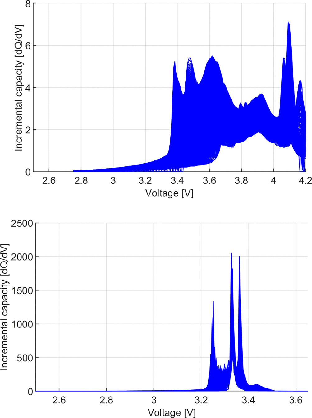
Figure 3. Training IC curves for NMC (up) and LFP (down) use case.
7.3 Model generation
The obtained IC curves were pre-processed to fit the format of the inputs of the training model.
The IC curves of the NMC use case are reduced to a voltage range of 3.3 V to 4.11 V. The IC curves were interpolated using a fixed voltage step to obtain a size of 200.
The IC curves of the LFP use case were reduced to a voltage range of 3.2 V to 3.5 V. The IC curves were interpolated using a fixed voltage step to obtain a size of 500.
The MLP was designed with one hidden layer of 10 neurons. This model was trained with the pre-processed 32768 samples (the IC curves) and their labels (the global degradation indicators
,
, and
) using a Bayesian regularization backpropagation process, which employs adaptive Levenberg–Marquardt optimization and therefore does not use a fixed learning rate. These samples were randomly divided into training (70 %), validation (15 %), and testing (15 %) subsets. Random weight initialization with different random seeds and repeated runs was applied to reduce the training variability. Nonlinear activation functions were used in the hidden layers, and both the inputs and targets were normalized prior to training using the selected training algorithm. The optimization was performed by minimizing the mean square error (MSE) loss function. A maximum of 1000 epochs were performed.
Figure 4 shows the evolution of the training metrics.
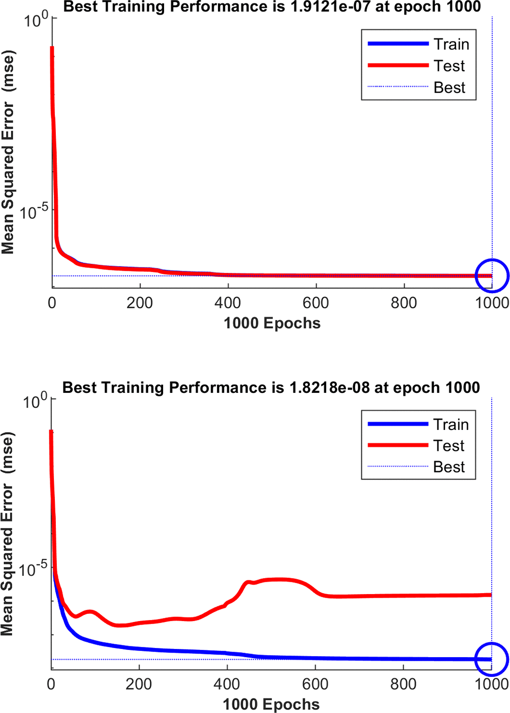
Figure 4. Training metrics for NMC (up) and LFP (down) use cases.
As a result, LLI and LAM quantification models of the NMC and LFP cells were generated. The obtained training error in the NMC use case is 0.19 microns and in the LFP use case 0.018 microns (range of 0 to 1, no unit).
7.4 Model verification
The models were verified using IC curves generated at the LLI and LAM values defined in
Table 5.
Table 5. LLI and LAM value range used to artificially generate IC curves for the verification.
| Name | Values |
|---|
| LLI | 0 | 0.01 | 0.03 | 0.05 | 0.07 | 0.12 |
| LAMpe lithiation | 0 | 0.01 | 0.03 | 0.05 | 0.07 | 0.12 |
| LAMpe delithiation | 0 | 0.01 | 0.03 | 0.05 | 0.07 | 0.12 |
| LAMne lithiation | 0 | 0.01 | 0.03 | 0.05 | 0.07 | 0.12 |
| LAMne delithiation | 0 | 0.01 | 0.03 | 0.05 | 0.07 | 0.12 |
In total, 7776 IC curves were generated. These IC curves are pre-processed as training curves (limited to the corresponding voltage ranges and interpolated with fixed voltage steps to obtain 200 values) and are passed to the model. A real vs. predicted graph of the LLI and LAM quantification models of the NMC and LFP use cases are shown in
Figures 5 and 6, respectively.
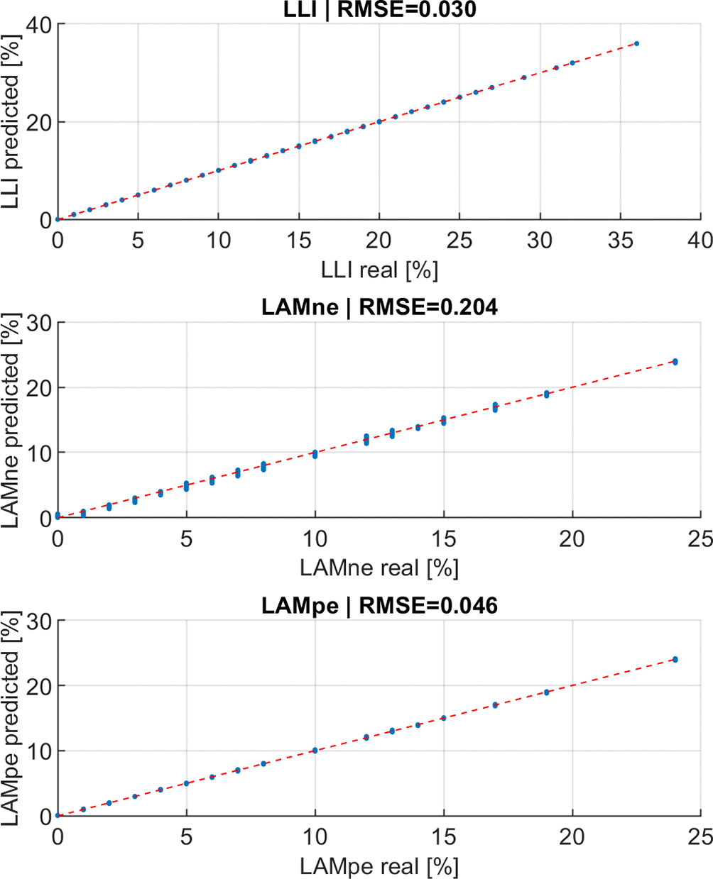
Figure 5. Real vs predicted graph of the LLI and LAM quantification model of the NMC use case in percentage.
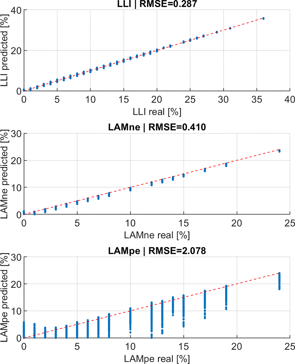
Figure 6. Real vs predicted graph of the LLI and LAM quantification models of the LFP use case in percentage.
7.5 Sorting results
IC curves of the first end-of-life batteries of the NMC and LFP use cases were obtained.
For the NMC use case, two modules of NMC cells of 12s2p configuration has been tested at a C/20 current rate from 3.0 V to 4.2 V. The NMC module was tested with a BMS, recording the 2p cell-level voltages.
The modules were tested under ambient conditions (23 ± 2 K). Cycling was performed using a calibrated EA-PSB 10200-420 bidirectional power supply. All the measurements were acquired via the module’s internal manager and transmitted over the CAN to the controller software on a desktop PC. A custom Python application then combines the incoming data with the test plan to control the power supply and handle data logging and storage.
The data were filtered. The repeated voltage measurements have been removed, the noise in the registered voltage has been smoothed with a moving average filter, and the voltage step has been set up to 0.01 V to interpolate the voltage and the charge capacity. Then, the IC curves were calculated and pre-processed to match the LLI and LAM quantification models, as shown in
Figure 7.
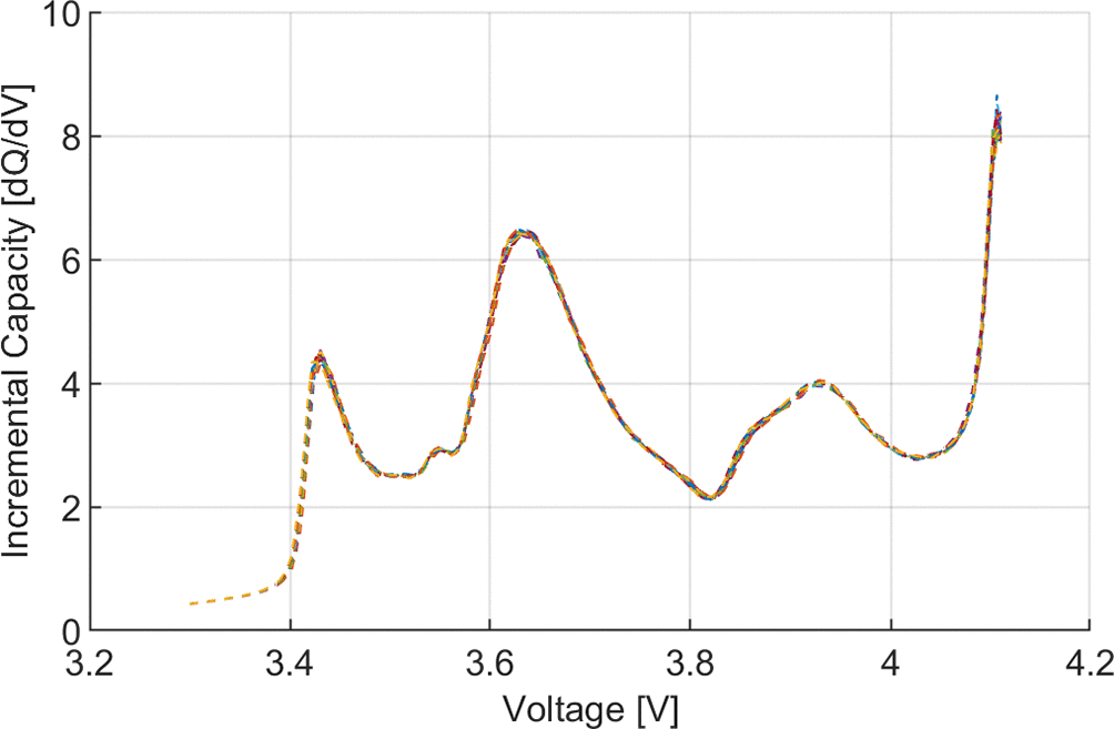
Figure 7. Validation IC curves of the 24 2p cells of NMC use case.
The results for the evaluated 24 NMC pseudo-cells (2p cell block) are shown in
Table 6.
Table 6. Results of the LLI and LAM quantification model for NMC use case.
| Cell name | LLI [%] | LAMne [%] | LAMpe [%] | SOH [%] |
|---|
| Mod01C001 | 2,71 | 14,09 | 6,82 | 93.98 |
| Mod01C002 | 2,95 | 13,30 | 6,70 |
| Mod01C003 | 3,21 | 12,59 | 6,73 |
| Mod01C004 | 2,18 | 12,12 | 7,26 |
| Mod01C005 | 3,04 | 13,38 | 6,36 |
| Mod01C006 | 2,89 | 13,20 | 6,71 |
| Mod01C007 | 2,91 | 13,98 | 6,66 |
| Mod01C008 | 2,85 | 13,23 | 6,81 |
| Mod01C009 | 2,87 | 13,49 | 6,68 |
| Mod01C010 | 2,76 | 13,82 | 6,50 |
| Mod01C011 | 2,53 | 14,19 | 6,35 |
| Mod01C012 | 2,26 | 13,49 | 6,40 |
| Mod02C001 | 2,57 | 14,71 | 6,47 |
| Mod02C002 | 2,68 | 13,88 | 6,77 |
| Mod02C003 | 3,12 | 13,34 | 6,41 |
| Mod02C004 | 2,43 | 14,06 | 7,15 |
| Mod02C005 | 2,88 | 13,91 | 7,05 |
| Mod02C006 | 2,95 | 13,89 | 6,89 |
| Mod02C007 | 2,88 | 13,71 | 7,10 |
| Mod02C008 | 2,96 | 13,47 | 7,38 |
| Mod02C009 | 3,17 | 13,02 | 7,48 |
| Mod02C010 | 2,99 | 14,03 | 7,20 |
| Mod02C011 | 2,96 | 14,08 | 7,36 |
| Mod02C012 | 2,77 | 13,68 | 7,24 |
For the LFP use case, a whole module of LFP cells of 16s1p configuration has been tested at a C/20 current rate from 46.3 V up to 58.4 V. Only the voltage at the module level is available. Therefore, it is assumed that the cells are in the same SOH and have the same level of LLI and LAM, and that they are perfectly balanced. Consequently, the module-level voltage profile was divided by 16 to obtain a representative voltage profile for all cells inside the module.
The module was tested using a Bitrode cycler at room temperature (25 Â °C). The initial results were verified through an analysis using Origin Lab software, where the correct behavior of all measured parameters was observed.
The data were filtered. Repeated voltage measurements were removed, and the voltage step was set to 0.001 to interpolate the voltage and charge capacity. Then, the IC curve was calculated and pre-processed to match the LLI and LAM quantification models, as shown in
Figure 8.
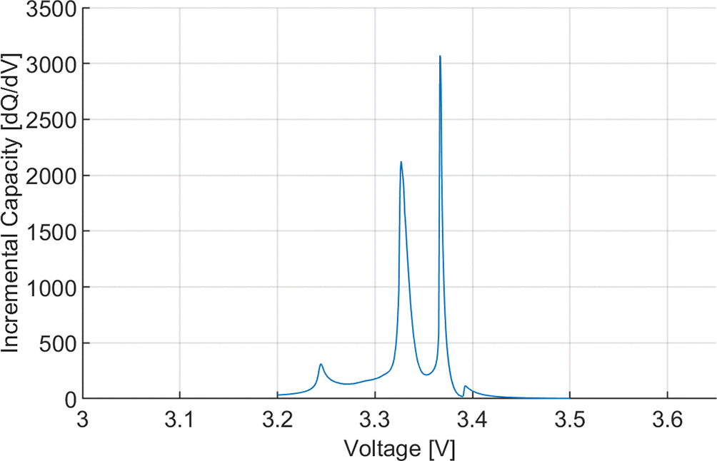
Figure 8. Validation IC curves of the module 16s1p configuration of LFP use case.
The results of the evaluated representative LFP cell is disclosed in
Table 7.
Table 7. Results of the LLI and LAM quantification model for LFP use case.
| LLI | LAMne [%] | LAMpe [%] |
SOH [%] |
|---|
| Representative cell | 0.96 | 2.95 | 8.11 | 98.48 |
8. Discussion
The generated coin cells (electrode vs. lithium) provide electrode-level information. The obtained voltage profiles were used to obtain the full-cell voltage profile (see Eq (3)). The adjusting parameters of this equation were optimized to fit the measured full-cell-level voltage profile. The fitting error in the NMC use case was higher (0.27) than that in the LFP use case (0.13). This reduced RMSE value indicates the effort invested in reducing the differences between synthetic data and experimental data through data curation. LFP cells have voltage plateaus that significantly affect the IC curves, and the reduction of this error along with the error in the IC curves (see
Figure 9) has been challenging.
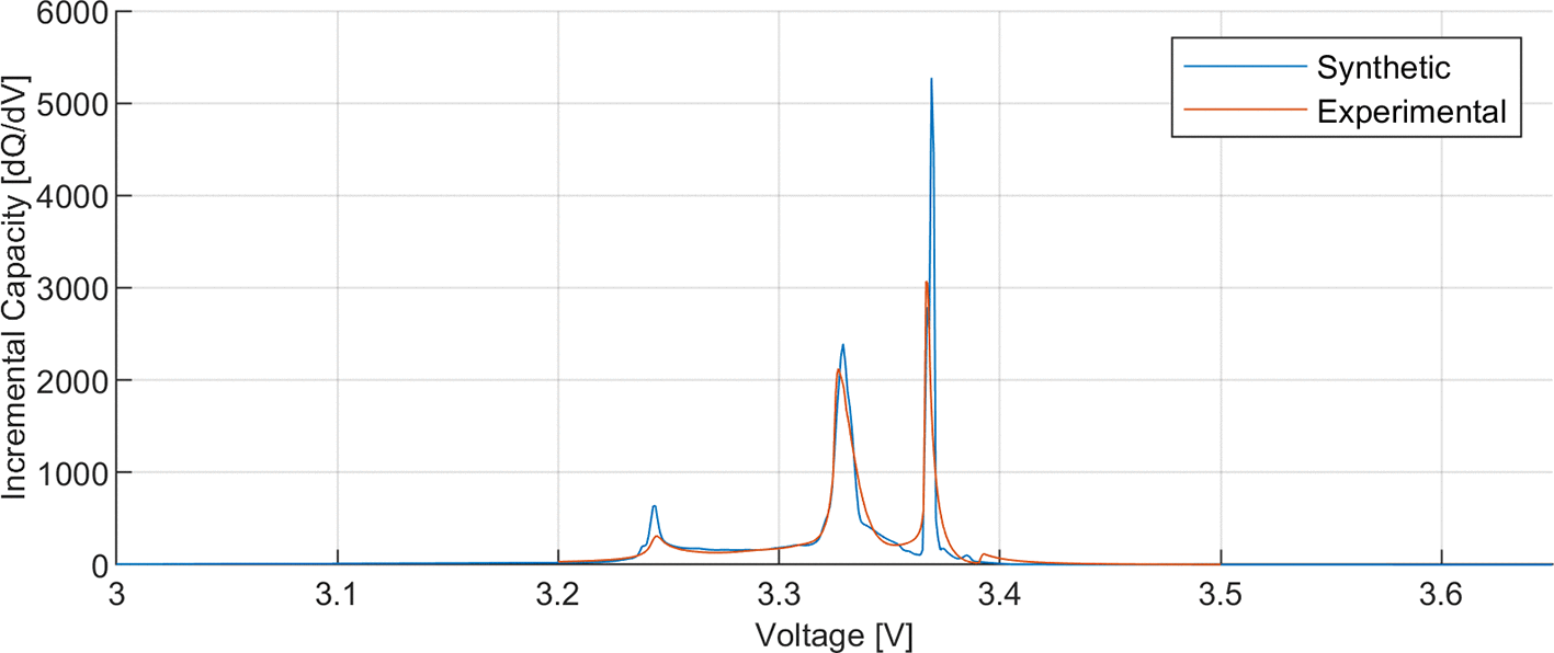
Figure 9. LFP use case's IC synthetic and experimental reference curves at BOL.
The artificially generated results are shown in Fig. 3. The characteristics for each case are not appreciable, however, it can be seen that the values do not suffer transformation out of the norm. There were no new peak generations with a drastic increase in some peaks. In addition, all the generated IC curves are representative of the actual IC curves that can be measured at different SOH values.17
The model generation metrics (
Figure 4) show the accuracy level of the model in the training and testing phases. The obtained values indicate an underfitting scenario. In addition, the flatness of the MSE value from 400 epochs onwards in both use cases shows that it is not likely to significantly improve the fitting when the epochs are increased. The results show that the selected configuration of the MLP is unlikely to improve with further training. Therefore, the training was considered satisfactory.
The model generation metrics in the LFP use case indicate that it is likely to suffer from overfitting. The testing error is significantly higher than the training error (at least 10 times higher), and there is an epoch from which, instead of reducing the test error, it increases.
Model verification shows that the NMC use case has a remarkable accuracy rate in the non-observed synthetic-generated IC curves. The RMSE error is below 0.3 in all cases. This low verification error shows the level of accuracy of a model that quantifies LLI and LAM using the IC curve as input. Nonetheless, the LFP use case showed lower accurate values, especially in LAM quantification. This is a sign of overfitting.
If we analyze the inherent characteristics of each cell chemistry, critical differences between both use cases can be seen, even though they are both lithium-based batteries. NMC cells have smoother voltage profiles than LFP cells, where there are no voltage plateaus that generate huge peaks in the IC curves. The maximum IC value of the evaluated NMC cells was < 10. Instead, the maximum IC value of the evaluated LFP cell was greater than 1000. In addition, the NMC IC curves exhibit wider peaks. The selected voltage step of the LFP IC curves was 1m V instead of the 10 mV selected for the NMC use case because of the required resolution to properly capture the peaks of the LFP. The first trial with a resolution of 10 mV showed that the peaks were deformed at reduced values. This fact points to a possible resolution problem in the LFP use case.
The generated models were tested with experimental IC curves of batteries sorted for second-life applications.
Training and verification of the NMC model showed that it was accurate with artificial data. The experimental data show a low level of LLI and a significant LAM in the positive electrode. The dominant aging mode is the LAM of the positive electrode, which represents capacity reduction at the cell level. The quantified ageing (6.35 %–7.48 %) and the measured ageing (6.02 %) differed by less than 1.5 %. This indicates the actual accuracy of the developed LLI and LAM quantification models.
However, the training and verification results of the LFP use case indicate overfitting issues. The results of applying the ML model to the LFP experimental data showed a difference greater than 5 %. Further work is required to generate LFP LLI and LAM quantification models. Overfitting, resolution problems, and the inherent characteristics of the LFP are key to solving the detected issues.
9. Conclusion
The methodology for generating LLI and LAM quantification models based on an MLP algorithm is presented. This methodology involves obtaining electrode-level data to generate the training data of the MLP model. These data are generated using the DEST tool, which induces LLI and LAM at the cell-level voltage owing to the obtained knowledge at the electrode level. This methodology was tested under two cases: the first with NMC cells and the second with LFP cells. The results showed an error below 1.5 % in the NMC use case and an error above 5 % in the LFP use case, validating the methodology (NMC use case) and highlighting the need for further work with the always challenging LFP technology.
In future work, first, the likely overfitting of the LFP use case will be addressed by normalizing the samples using minimum and maximum values and the z-score. Second, a deeper analysis of the resolution problem in the LFP use case will be performed. The minimum resolution required to describe the LFP IC high peaks, but still not producing too many points to avoid numeric noise, will be analyzed in detail. Finally, the half-cell data quality improvement will be researched to reduce the error committed by the experimental data.
Ethics and consent
Ethical approval and consent were not required.
References
- 1.
Parvizi P, Jalilian M, Amidi AM, et al.:
From Present Innovations to Future Potential: The Promising Journey of Lithium-Ion Batteries.
Micromachines.
Feb. 2025; 16(2). PubMed Abstract
| Publisher Full Text
| Free Full Text
- 2.
Guan S, Tong H, He Z, et al.:
Status, challenges, and techniques of echelon utilization of retired lithium-ion batteries.
J. Energy Storage.
Oct. 2025; 132: 117786. Publisher Full Text
- 3.
Underwriters Laboratories:
UL 1974, the Standard for Evaluation for Repurposing Batteries.
ANSI/CAN/UL 1974.
2018; 2018.
- 4.
Ahmeid M, Muhammad M, Lambert S, et al.:
Data-driven classification of lithium-ion batteries for second-life applications.
J. Energy Storage.
Oct. 2025; 133: 117994. Publisher Full Text
- 5.
Mowri ST, Barai A, Sheikh M, et al.:
Dataset for assessing the impact of first-life lithium-ion battery degradation on second-life performance.
Data Brief.
Dec. 2025; 63: 112208. PubMed Abstract
| Publisher Full Text
| Free Full Text
- 6.
Rehman S, Al-Greer M, Burn AS, et al.:
High-Volume Battery Recycling: Technical Review of Challenges and Future Directions.
Batteries.
Feb. 2025; 11(3). Publisher Full Text
- 7.
Wu Q, Ye W, Liang R, et al.:
Two-Step Sorting and Regrouping Method of Retired Lithium-Ion Battery Cells Based on Branches’ Topological Structures.
Energy Fuel.
Nov. 2024; 38(21): 21122–21133. Publisher Full Text
- 8.
Rajaeifar MA, Ghadimi P, Raugei M, et al.:
Deep sorting of reused batteries for enabling long-term consistency grouping with unknown prior conditions.
Cell Rep. Phys. Sci.
Jul. 2025; 6(7): 102657. Publisher Full Text
- 9.
Zeng J, Liu S:
Research on aging mechanism and state of health prediction in lithium batteries.
J. Energy Storage.
Nov. 2023; 72: 108274. Publisher Full Text
- 10.
Jeon DH, Kim S, Hempelmann R:
State-of-the-art review of degradation mechanisms of commercial lithium-ion batteries.
J. Power Sources.
Aug. 2025; 646: 237242. Publisher Full Text
- 11.
Xu W, et al.:
Investigation of lithium-ion battery degradation by corrected differential voltage analysis based on reference electrode.
Appl. Energy.
Jul. 2025; 389: 125735. Publisher Full Text
- 12.
Mongkoltanatas J, Sahapatsombut U, Lailuck V, et al.:
Incremental Capacity Analysis of Lithium-Ion Batteries under Cyclic and Calendar Aging.
2024 International Conference on Materials and Energy: Energy in Electrical Engineering, ICOME-EE 2024.
2024. Publisher Full Text
- 13.
Arrinda M, et al.:
Application Dependent End-of-Life Threshold Definition Methodology for Batteries in Electric Vehicles.
Batteries.
Feb. 2021; 7(1): 12. Publisher Full Text
- 14.
Méndez-Corbacho FJ, Nieto-Castro D, Moreno-Artabe I, et al.:
DEST: A Simplified Model and Automated Tool for Loss of Lithium Inventory and Loss of Active Material Estimation in Li-ion Batteries**.
ChemElectroChem.
Mar. 2024; 11(5): e202300830. Publisher Full Text
- 15.
Zhang S, Zhai B, Guo X, et al.:
Synchronous estimation of state of health and remaining useful lifetime for lithium-ion battery using the incremental capacity and artificial neural networks.
J. Energy Storage.
Dec. 2019; 26: 100951. Publisher Full Text
- 16.
Hamed H, Yusuf M, Suliga M, et al.:
An Incremental Capacity Analysis-based State-of-health Estimation Model for Lithium-ion Batteries in High-power Applications.
Batter. Supercaps.
Sep. 2023; 6(9): e202300140. Publisher Full Text
- 17.
Dubarry M, et al.:
Identifying battery aging mechanisms in large format Li ion cells.
J. Power Sources.
2011; 196(7): 3420–3425. Publisher Full Text
- 18.
Arrinda M:
ICA curves of NMC and LFP cells at different LLI and LAM.
Zenodo.
Jul. 2026. Publisher Full Text
- 19.
Arrinda M:
marrinda/LIB-degradation-mode-quantification: LIB degradation mode quantification model generation.
Zenodo.
2026. Publisher Full Text