1. Introduction
Accurately forecasting the progression of solid tumors and predicting therapeutic outcomes for individual patients remains a major challenge. As in other complex and dynamic systems such as climate processes1,2 and financial markets,3 mathematical modeling offers a quantitative framework to describe and predict cancer behavior. This concept forms a central pillar of the field of mathematical oncology.4,5 Mathematical models of tumor growth have enhanced the understanding of cancer biology6–8 and are widely used to optimize treatment strategies, including chemotherapy9,10 and immunotherapy.11,12 They have also improved drug dosing design13,14 and supported the identification of potential biomarkers of treatment response.15
The foundations of tumor growth modeling trace back to Gompertz’s 1825 work on population dynamics16 and were later extended by von Bertalanffy’s growth theory.17 Applied to cancer, these ideas led to models that describe tumor development, estimate growth rates, and predict progression across tumor types.18,19 Classical approaches, including Gompertz, von Bertalanffy, exponential, and logistic models, have since been developed to characterize tumor growth behavior.20 Exponential models represent unrestricted growth or decay, whereas logistic and Gompertz models describe sigmoidal growth. These frameworks incorporate a biological carrying capacity to account for microenvironmental limitations, such as nutrient and oxygen availability, angiogenesis, space constraints, and immune responses, thereby capturing the experimentally observed reduction in growth rate as tumor size increases.18,21 Owing to their ability to represent constrained tumor growth, the Gompertz and von Bertalanffy models have often provided more accurate descriptions of tumor volume dynamics than exponential models.22 A comprehensive summary of the basic mathematical models used to describe tumor growth is presented in.23,24
A main objective of mathematical oncology is to understand and optimize cancer treatments by simulating tumor responses to therapy and the influence of treatment strategies on tumor–immune dynamics.25–29 These frameworks have been widely applied to improve treatment design, including chemotherapy, immunotherapy, combination therapies, and personalized dosing strategies aimed at enhancing therapeutic efficacy and overcoming resistance.30–37
Despite these advancements, accurately quantifying the efficacy of anticancer therapies from longitudinal tumor growth experiments remains a major challenge. Since treatment response is primarily evaluated through serial tumor volume measurements, the intrinsic biological variability and experimental noise associated with these data limit the reliability of conventional mathematical modeling approaches. Standard monitoring relies on discrete measurements over time,
, which do not strictly follow a smooth functional form due to both measurement noise and underlying biological variability. These fluctuations arise from experimental uncertainties, such as caliper positioning errors, variations in skin tension over subcutaneous tumors, and geometric approximations of irregular tumor shapes, as well as genuine short-term biological dynamics in tumor growth, making the resulting
data inherently non-smooth.38 A further limitation is the common use of single “endpoint” measures, such as the final tumor volume
, to judge treatment success.39 From a dynamical systems point of view, this is a very simplified description of the process, because it reduces the full-time evolution to one value. As a result, important information about how the tumor changes over time is lost, and different growth patterns can lead to the same final volume even if they respond very differently to treatment during the study. Therefore, there is a clear need for models that describe the full-time course of tumor growth rather than only its final state.
Previous studies have employed the area under the tumor growth curve (AUC) as a single summary measure of cumulative tumor burden for comparing treatment groups, emphasizing its ability to condense the entire tumor growth trajectory into a single numerical endpoint.40,41 More recently, Patten et al. systematically evaluated the statistical performance of AUC relative to other tumor-growth endpoints and demonstrated that its use as a descriptive summary statistic does not outperform simpler measures such as final tumor volume or change from baseline.42 These observations suggest that the principal limitation lies not in the cumulative information contained within the area under the tumor growth curve (AUC), but rather in its conventional use as a retrospective statistical endpoint that does not fully exploit the temporal evolution of tumor response. Consequently, although the AUC provides a useful summary of therapeutic efficacy, it offers limited insight into the dynamic progression of treatment response throughout the course of therapy. To overcome this limitation, the present study introduces a medical engineering framework for quantitative assessment of tumor treatment response based on cumulative tumor dynamics. Instead of directly modeling the raw tumor volume trajectory,
, the proposed methodology transforms longitudinal tumor measurements into a cumulative tumor burden function,
, obtained through temporal integration. This cumulative representation serves as the primary dynamic variable of the framework, providing a robust description of treatment response while reducing the influence of experimental variability. Importantly, the conventional AUC is naturally recovered as the terminal value of the cumulative function at the end of the observation period, thereby establishing a direct connection between the proposed dynamic formulation and the widely used cumulative treatment metric.
To establish a quantitative description of cumulative tumor dynamics, a variational formulation is introduced that assigns a scalar functional to the complete tumor trajectory by accounting for both tumor burden and its temporal evolution. This formulation enables comparison of entire longitudinal tumor trajectories rather than isolated measurements obtained at individual time points. Under the assumption of weak perturbations and linear coupling between treated and untreated tumors, the proposed framework demonstrates that differences in therapeutic response can be expressed through cumulative quantities directly related to the conventional AUC. Consequently, the AUC is reinterpreted from a post hoc statistical summary to the terminal state of a continuous dynamical process describing the cumulative evolution of therapeutic response over time.
Because tumor response to therapy frequently involves multiple biological phases, a single scaling behavior is often insufficient to accurately describe the underlying dynamics. Early after treatment, transient biological processes such as inflammation, edema, or tissue remodeling may temporarily increase the apparent tumor burden before sustained therapeutic effects become dominant. To capture these complex response patterns while preserving the scale-invariant structure of the cumulative formulation, a second-order Euler–Cauchy differential equation is introduced. The resulting solution represents cumulative treatment response as the superposition of two independent dynamical modes, allowing the framework to simultaneously describe early transient responses and long-term tumor suppression, stabilization, or regression within a unified mathematical formulation.
The proposed framework was evaluated using experimental breast cancer models subjected to photodynamic therapy (PDT), treatment with the mechanotherapeutic agent tranilast, conventional chemotherapy with doxorubicin, and combination therapy comprising tranilast and doxorubicin.43–45 In this study, tranilast was employed as a tumor microenvironment (TME)-modulating agent to alleviate desmoplasia through collagen depletion and the associated reduction in tumor stiffness.46 These case studies demonstrate the capability of the proposed cumulative dynamics framework to provide a unified quantitative methodology for evaluating diverse therapeutic strategies, supporting longitudinal treatment-response assessment and facilitating the development of predictive tools for preclinical and translational oncology.
2. Materials and Methods
2.1 Temporal integration for filtering experimental data
Let
denote the measured tumor volume as a function of time. To obtain a cumulative representation of tumor burden, the time series is transformed into its temporal integral,
(1)
which represents the area under the tumor volume–time curve (AUC). This transformation is used in place of the raw measurements
for subsequent analysis.
2.2 Generic formulation of treatment effects
Tumor dynamics were represented by two cumulative trajectories corresponding to untreated controls,
, and treated tumors,
. Treatment effects were quantified through the deviation between these trajectories rather than through isolated endpoint measurements. This cumulative representation was adopted to account for the full temporal evolution of tumor burden during the observation period. To characterize the overall behavior of tumor growth, a functional (
) depending on both tumor volume and its temporal variation was introduced. The functional was designed as a global descriptor of the tumor trajectory, incorporating information on tumor burden, growth dynamics, and temporal regularity. In contrast to endpoint-based metrics, which depend only on the final tumor volume, the proposed formulation evaluates the complete growth trajectory and therefore preserves information regarding the timing and evolution of treatment responses. The framework considers both untreated and treated tumor evolution as perturbations of a common dynamical system. Under the assumptions of weak treatment-induced perturbations and linear coupling between treatment action and tumor volume, the deviation of the functional can be expressed in terms of cumulative quantities associated with the tumor trajectory. In this regime, the leading-order treatment effect becomes proportional to the AUC of the tumor volume, providing a theoretical basis for using AUC as a descriptor of cumulative therapeutic exposure and treatment-induced trajectory modification. The mathematical formulation of the functional, the perturbation analysis, and the derivation linking functional deviations to the AUC are presented in the Results section.
2.3 Euler–Cauchy formulation
The cumulative framework provides a global description of treatment effects through deviations between treated and untreated tumor trajectories. To further characterize the temporal evolution of treatment effects, a power-law formulation was adopted. In its simplest form, the model generates a response that satisfies the condition of zero treatment effect at the onset of therapy. This formulation is primarily intended to describe the early stages following treatment initiation, during which tumor dynamics may exhibit rapid temporal changes. To account for more complex response patterns, a second-order Euler–Cauchy differential equation was also introduced. The resulting solution consists of a superposition of two independent power-law modes, enabling the representation of distinct dynamical components operating over different time scales. This formulation preserves scale invariance while remaining consistent with the cumulative AUC-based framework adopted in the present study.
2.4 Animal models, experimental protocols and data
All animal experimental procedures were approved by the Cyprus Veterinary Services, the national authority responsible for monitoring animal research (license numbers: CY/EXP/PR.L09/2025, CY/EXP/PR.L2/2025). The number of animals per experimental group was determined during the ethical approval process in accordance with the 3Rs principles (Replacement, Reduction and Refinement), ensuring the minimum number of animals necessary for the objectives of the study. Animals were housed at the Transgenic Mouse Facility of the Cyprus Institute of Neurology and Genetics (Nicosia, Cyprus) under specific pathogen-free conditions and routine veterinary supervision, in accordance with Cyprus Law N.55(I)/2013 and EU Directive 2010/63/EU. Breast tumor models were generated by implanting 5 × 10⁴ E0771 cells into the left flank or the third mammary fat pad of 6–8-week-old C57BL/6 mice, respectively. Tumor volume was calculated from caliper measurements according to
where
and
denote the longest and shortest perpendicular tumor diameters, respectively. Animals were allocated to experimental groups using a computer-generated random sequence. No blinding was performed during allocation, conduct of the experiments, outcome assessment, or data analysis. No formal protocol registration was performed. When tumors reached approximately 100 mm3, 5-aminolevulinic acid hydrochloride (5-ALA; MedKoo Biosciences) was administered by intratumoral injection at a dose of 50 mg/kg.47 Prior to injection, the tumor area was shaved and disinfected with an antiseptic solution. Intratumoral injection was performed using a sterile syringe fitted with a fine needle, such as a 29G needle. The needle was carefully inserted into the center of the tumor mass to promote homogeneous distribution of 5-ALA within the tumor. The injection was carried out slowly to minimize leakage, tissue disruption, or local damage. Animals were closely monitored during and after the procedure. Two hours after 5-ALA administration, tumors were irradiated using a red laser at 639 nm (PL252, 4.5 mW) to deliver a total light dose of 40 J/cm2.47 PDT was performed three times per week for two weeks.48,49 Treatments were administered to groups of 3–4 mice, including: (i) saline-treated control, (ii) laser-only treatment, and (iii) PDT treatment.50 Animals were monitored throughout the study for tumor growth and general health status. Experiments were conducted within predefined ethical limits, and animals were euthanized when required according to approved welfare protocols. The experimental protocol above is also presented in Figure 1. In addition, experimental data from51 were included in the current study. In this study, orthotopic breast tumors were established by implanting 5 × 10⁴ E0771 cells into the third mammary fat pad of 6–8-week-old C57BL/6 mice. When tumors reached approximately 200 mm3, three treatment cycles were administered to groups of 3–4 mice. The treatment groups included saline control, Tranilast, and the combination of doxorubicin with Tranilast. Tumors were surgically excised one day after administration of the third doxorubicin dose, after which the abdominal wall and skin were sutured, and animals were monitored for survival analysis. Survival was defined as the time from treatment initiation until death. Mice were euthanized by CO2 inhalation when required.
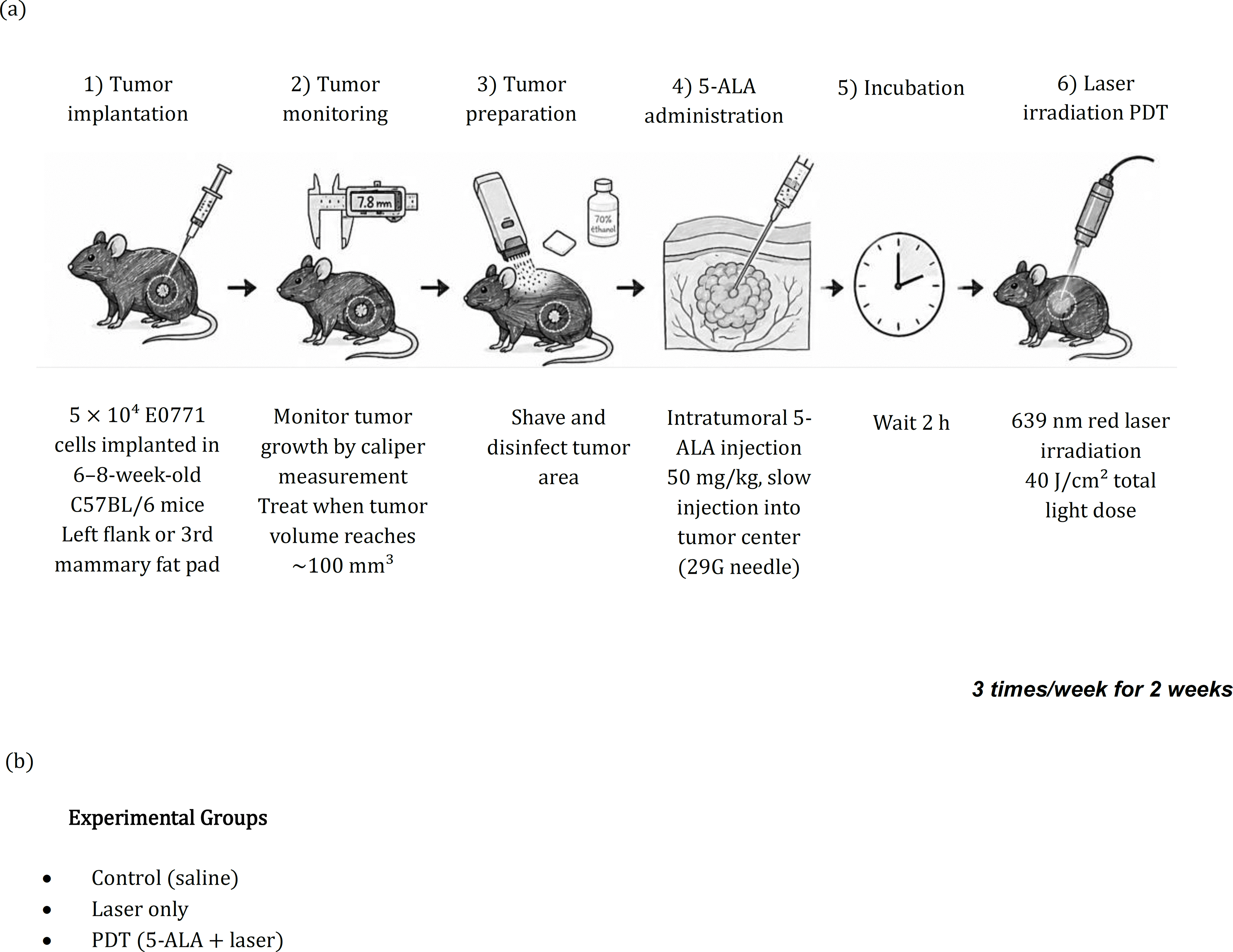
Figure 1. (a) Experimental timeline of the murine photodynamic therapy (PDT) protocol. E0771 breast tumors were established in C57BL/6 mice and monitored by serial caliper measurements. When tumors reached approximately 100 mm3, mice received an intratumoral injection of 5-aminolevulinic acid (5-ALA; 50 mg/kg), followed 2 h later by irradiation with a 639 nm red laser (40 J/cm2). PDT was administered three times per week for two weeks. Tumor progression was monitored throughout the study, and treatment efficacy was evaluated by comparing the saline-treated control, laser-only, and PDT groups. (b) The experimental groups used in this paper.
3. Results
This section presents the main theoretical developments and experimental validation of the proposed cumulative modeling framework. First, the mathematical properties of the cumulative formulation are analytically investigated to establish its theoretical basis and demonstrate its advantages over conventional tumor volume analysis. Subsequently, the proposed dynamical framework is developed and its predictive capability is evaluated using representative preclinical tumor growth datasets.
3.1. Theoretical Justification of Temporal Integration as a Noise Filter
To establish the theoretical foundation of the proposed cumulative framework, we first investigate the statistical properties of the cumulative tumor burden function and analytically examine its response to measurement noise. The measured volume of the tumor
as a function of time is modeled as the sum of a deterministic component and an additive stochastic perturbation:
(2)
where
represents the underlying (latent) tumor volume evolution, and
denotes the measurement-noise associated with the experimental procedure. This measurement noise is attributed to external, non-biological sources, including variability in caliper positioning, localized skin-tension effects over subcutaneous tumors, and geometric approximations required for irregular tumor morphologies as already mentioned in the introduction. These effects are assumed to introduce no systematic temporal drift and to fluctuate randomly about the underlying tumor volume. Accordingly, the noise is modeled as a zero-mean, temporally uncorrelated stochastic process. The smoothing effect of integration becomes apparent when considering the cumulative integral of the measured volume. Integration acts as a low-pass filtering operation over the interval
, emphasizing low-frequency trends while attenuating the relative influence of high-frequency fluctuations. Consequently, positive and negative noise contributions tend to partially cancel over the integration interval, reducing their relative impact on the cumulative quantity. According to
Equation (2), the measurement error at time
is given by
(3)
The noise process is assumed to have zero mean:
(4)
and constant variance (which implies that the magnitude of the measurement uncertainty does not depend on time):
(5)
where
denotes the standard deviation of the measurement noise and therefore the standard deviation (measurement error) is:
(6)
In addition, the noise is assumed to be uncorrelated in time, such that:
(7)
To investigate the effect of temporal accumulation on the measurement noise, the cumulative integral of the signal is introduced. Let
denote the observation interval. The tumor volume is assumed to be a continuous, non-negative function of time:
(8)
We define two fundamental functionals. First the endpoint functional:
(9)
Second, the cumulative burden functional given by Equation (1).
Equation (1) represents the area under the
curve in the domain
. To visually and geometrically appreciate why the cumulative signal
exhibits a significantly smoother profile than the raw volumetric data
, one must analyze the temporal evolution of their respective noise structures. In the primary
domain, the measurement noise variance
remains constant over time (Equation 5). Consequently, the raw data is subjected to persistent stochastic fluctuations at every sampling interval
. Because these high-frequency perturbations do not decay or correlate, the measured
trajectory retains a jagged appearance throughout the observation period. Conversely, the cumulative signal given by Equation (1) continuously aggregates the measurements over time. If
, then
reduces to the AUC functional defined previously. Using Equations (1),(2) the signal decomposition yields:
(10)
or,
(11)
where,
(12)
and,
(13)
The statistical properties of
are therefore determined by the integrated noise term
(Equation (13)), whose accumulation governs the residual variability of the cumulative signal. In a finite-resolution measurement with sampling interval
, the integral is approximated as:
(14)
where,
(15)
The noise contribution becomes:
(16)
The second moment of
is:
(17)
An expansion of Equation (17) leads to (see Appendix A):
(18)
where,
and
. Using
Equation (6) across all terms (see Appendix A),
(19)
By substituting
in
Equation (19) we conclude in:
(20)
Since
is fixed by the acquisition system:
(21)
Thus,
(22)
Since tumors often exhibit accelerating growth during the early stages of development, we can assume that:
(23)
where
, and
is a positive arbitrary constant, thus:
(24)
Thus, the relative noise-to-signal ratio decreases with time:
(25)
Therefore, although the absolute uncertainty of the integrated noise increases proportionally to
, the deterministic cumulative signal increases proportionally to
. Consequently, the relative contribution of the stochastic component decreases with increasing observation time, resulting in a progressively smoother cumulative trajectory.
Furthermore, integration accumulates the entire volumetric history rather than relying on isolated measurements, reducing the influence of transient fluctuations such as localized swelling, tissue necrosis, or other short-term biological variations. Consequently, the cumulative signal provides a more robust representation of the dominant long-term tumor dynamics than the raw volume time series. The overall procedure and an example using simulated
and
data is presented in Figure 2.
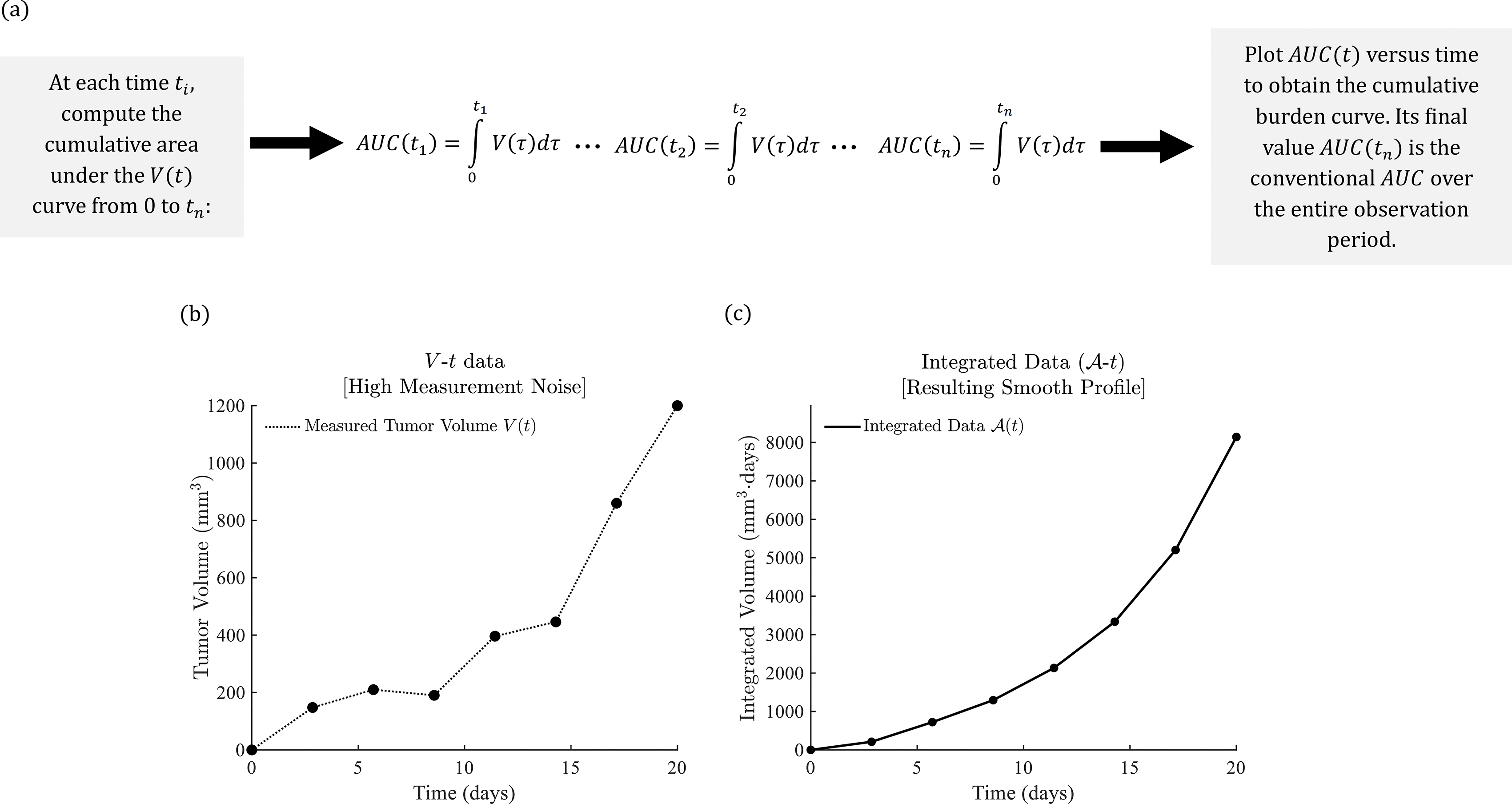
Figure 2. (a) The overall procedure for deriving the AUC-t graph. (b) A simulated raw
profile constructed from eight discrete observations. The data exhibits severe, chaotic fluctuations due to constant, uncorrelated experimental measurement noise, which obscures the underlying growth trend. (c) The corresponding
profile generated by calculating the cumulative integral of the raw data. Despite the massive noise present in the initial inputs, the integrated trajectory displays a highly stabilized, smooth geometric profile, illustrating the error-canceling property of temporal accumulation.
3.2. Modelling of treatment effects
We consider two regimes. First, the control (unperturbed) system, in which the tumor evolves according to its intrinsic biological dynamics:
(26)
where,
is the tumor volume at time
in the control case,
is the initial tumor-volume function from which the evolution starts,
is an operator describing the natural dynamics of the tumor. Second, we consider the perturbed system:
(27)
where
represents therapy-induced deviation from the natural trajectory. We introduce a biologically motivated action-like functional defined on tumor trajectories:
(28)
where
is a function that depends on the tumor volume, its rate of change, and time. Unlike endpoint measurements, which summarize only specific aspects of tumor growth,
incorporates information from the entire tumor trajectory. Consequently, it can capture features of tumor evolution such as growth intensity, temporal variability, and trajectory smoothness. In this study,
is introduced as a global measure of tumor-growth dynamics rather than as a quantity derived from a variational principle. A general form is given by:
(29)
where
is a positive weighting parameter and
is a function describing the contribution of tumor volume and time to the overall growth metric. The term
is analogous to kinetic energy in classical mechanics and quantifies the dynamical activity of tumor growth, whereas
plays a role analogous to potential energy and represents the contribution of tumor size and biological constraints. The functional
therefore characterizes both the magnitude and the temporal evolution of the tumor trajectory. The specific form of
depends on the biological processes under consideration and may incorporate intrinsic growth mechanisms, carrying-capacity effects, nutrient availability, immune response, or external interventions. A useful decomposition is
(30)
where
, describes intrinsic tumor-growth dynamics and
represents time-dependent external influences such as therapeutic interventions. Under this decomposition, tumor evolution in the absence of treatment is characterized by the control functional:
(31)
which depends only on the intrinsic biological contribution
and the trajectory-regularity term
When treatment is applied, the tumor dynamics are described by the perturbed functional:
(32)
where
represents the influence of treatment on tumor growth and introduces an explicit time-dependent external contribution to the tumor trajectory. We define the functional deviation:
(33)
which quantifies the cumulative effect of treatment on the tumor-growth dynamics over the observation interval. Using a Taylor series expansion of
around
:
(34)
Assume a weak perturbation regime, where:
. In this case,
(35)
Thus:
(36)
The simplest approach is to assume a linear coupling approximation for simplicity:
(37)
Where
is the effective time-dependent treatment efficacy. By substituting
Equation (37) to
Equation (36) it is concluded:
(38)
To simplify this expression, we apply the weighted mean value theorem for integrals, which states that if
and
is continuous, then there exists a value
in the range of
such that52:
(39)
showing that the effect of the treatment reduces, in an averaged sense, to a scaling of the classical AUC functional. In particular, if
varies slowly over the interval
, it can be approximated by a constant representative value, denoted by
. This leads directly to the same reduced form, in which the cumulative tumor burden (AUC) becomes the dominant quantity, modulated by the average strength of the external perturbation. Thus:
(40)
This result shows that the AUC is a linear functional of the tumor trajectory, that therapeutic effects accumulate over time, and that the action-like deviation is proportional to the cumulative tumor burden. However, it is important to note that the AUC does not replace the full dynamics, but acts as a first-order sufficient descriptor of cumulative exposure under linear perturbation assumptions.
Using concepts inspired by classical mechanics, the proposed framework shows that, under a weak perturbation regime and linear coupling assumptions, the leading-order functional deviation is proportional to the Area Under the Tumor Growth Curve (AUC). In this formulation, a regularity term governed by α accounts for temporal variations in tumor growth, while the AUC emerges as the dominant descriptor of cumulative treatment exposure. Furthermore, the analysis demonstrates that endpoint measurements,
, do not uniquely characterize tumor evolution, since different growth trajectories may lead to the same final tumor volume. As a result, endpoint metrics discard information about the intermediate dynamics of tumor growth. In contrast, the treatment-induced functional deviation depends on the entire tumor trajectory through its cumulative history. Therefore, under weak perturbations and linear coupling between treatment and tumor volume, the deviation of the action-like functional induced by external interventions is proportional to the AUC. This establishes the AUC as a first-order descriptor of cumulative treatment effects, whereas endpoint measurements capture only the final state of the underlying dynamical process.
3.3. The Euler Cauchy Equation to quantify treatment effects
The previous section established that, under a weak perturbation regime and linear coupling between treatment efficacy and tumor volume, the treatment-induced functional deviation is proportional to the AUC. Consequently, the cumulative quantity:
(41)
may be viewed as a first-order descriptor of the overall treatment effect. Thus,
(42)
where,
represent the volumes of the control and treated samples respectively. We assume that the underlying dynamics are scale-invariant, in the sense that no intrinsic time scale is introduced by the governing equation. This assumption is motivated by the observation that tumor growth can often be approximated by power-law behavior over finite time intervals (
Equations (23),
(24)). The simplest first-order scale-invariant differential equation satisfying this requirement is:
(43)
where,
, and
are arbitrary constants. This equation generates power-law solutions and therefore provides the simplest dynamical description of the accumulation of treatment effects. In particular,
Equation (43) can be solved using variable separation (Appendix B) leading to the following solution:
(44)
where,
an arbitrary constant and
(
). If the tumor volume is normalized as
where
the tumor volume at
(defined as the day on which therapy begins), then
for both control and treated samples. Therefore at
it should be
.
Equation (44) satisfies this requirement. Despite its simplicity and biological relevance, the first-order model possesses only one independent solution. Consequently, it predicts a single power-law exponent and cannot accommodate more complex growth patterns. Experimental tumor-volume data often exhibit deviations from a pure power law. These observations suggest that a single power-law mode may be insufficient to describe the entire growth process. To accommodate such behavior while preserving scale invariance, a second-order extension is introduced, leading naturally to the Euler–Cauchy equation:
(45)
The term
is not introduced arbitrarily; rather, it represents the simplest extension of the first-order scale-invariant model that preserves the same dimensional structure and invariance properties while increasing the number of independent solutions from one to two.
The solution of
Equation (45) (see also Appendices C, D) is presented below:
(46)
where,
are arbitrary constants.
Equation (46) also satisfies the initial condition
.
Equation (46) shows that the Euler–Cauchy model describes tumor growth as a superposition of two independent power-law modes. One mode may represent the dominant long-term growth trend, whereas the second mode acts as a correction that captures deviations from simple power-law behavior. Consequently, the inclusion of the term
provides the minimum additional flexibility required to describe more complex tumor-growth dynamics while preserving the scale-invariant structure of the original first-order model.
Figure 3 illustrates several characteristic profiles generated by the Euler–Cauchy solution (Equation 46) where
denotes the treatment effect, defined as the difference between the area under the curve (
) of the treated and control groups. Positive values of
indicate a beneficial therapeutic response, whereas negative values indicate an adverse response, such as treatment-induced inflammation, edema, swelling, or other transient side effects that temporarily outweigh the therapeutic benefit. All curves satisfy the initial condition (
), implying that no treatment effect is present at the initiation of therapy. The subsequent evolution is determined by the interaction of two power-law modes characterized by the exponents
and
. Several biologically relevant behaviors emerge naturally from this model. In the simplest case,
remains positive for all times, corresponding to a treatment that produces an immediate and continuously increasing therapeutic benefit. Other parameter combinations generate an approximately linear initial phase, which may represent a constant-rate accumulation of treatment efficacy during the early stages following administration. Of particular interest is the case in which
initially becomes negative before eventually attaining positive values. This behavior arises when the lower-order power-law component dominates at early times and the higher-order component becomes dominant at later times. Biologically, such a response may correspond to therapies that initially induce local tissue reactions, inflammatory responses, edema, or transient swelling. During this phase, the measured treatment effect appears unfavorable and
becomes negative. As the therapeutic mechanism progressively develops, the beneficial component of the response increases and eventually exceeds the adverse effects, causing the treatment-effect curve to cross the zero axis. The crossing point represents a critical transition from net adverse response to net therapeutic benefit. The minimum of the curve corresponds to the time at which the adverse effects are most pronounced. Following this point, the treatment effect increases as the therapeutic mechanisms become dominant. The subsequent rapid growth of
indicates increasing efficacy and may reflect cumulative biological processes such as drug accumulation, delayed activation of therapeutic pathways, immune-mediated responses, or progressive suppression of disease activity.
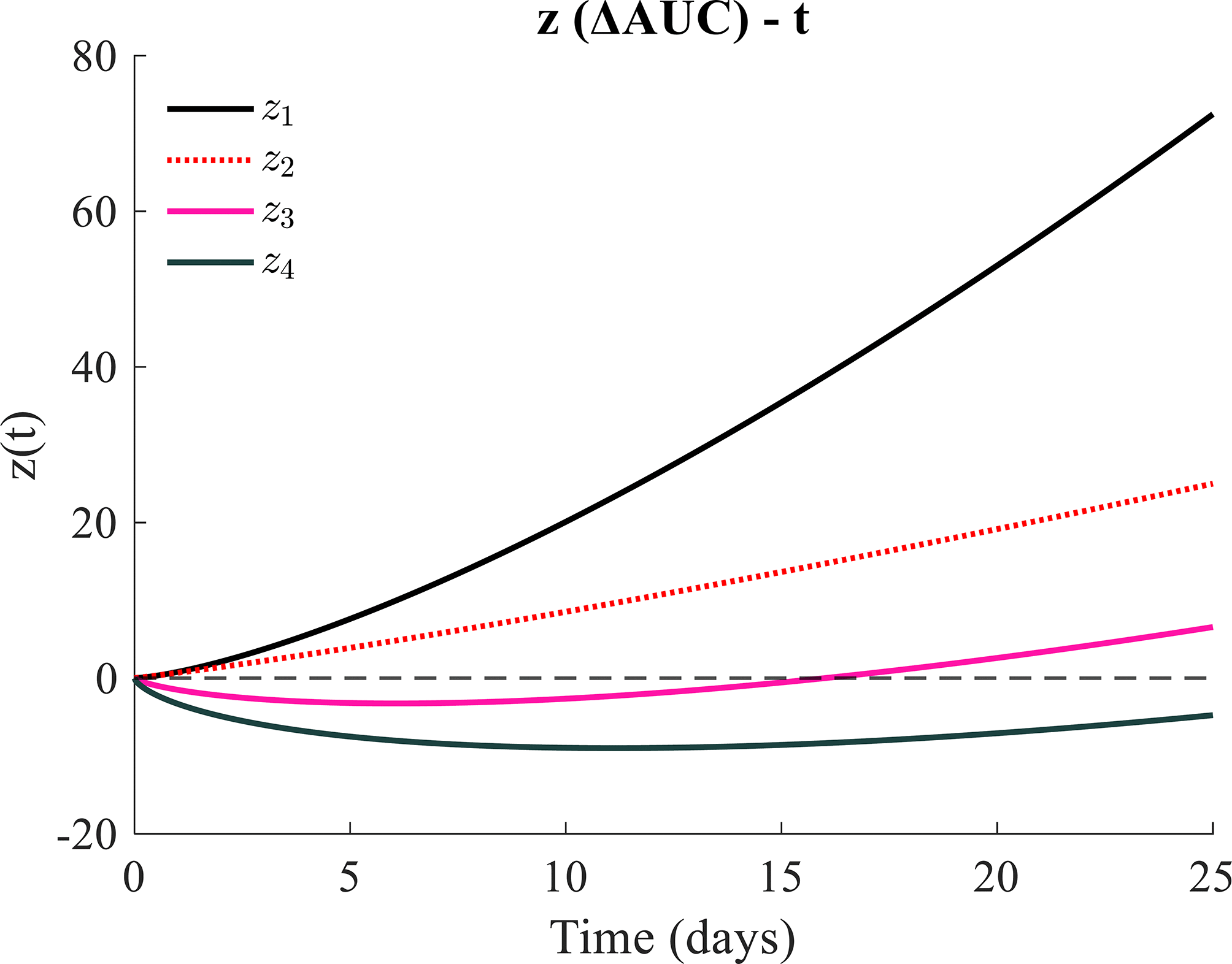
Figure 3. Simulated characteristic temporal profiles generated by the Euler–Cauchy solution (Equation 46), where
denotes the treatment effect defined as the difference between the AUC of the treated and control groups over a 0–30 day interval. Positive values indicate a beneficial response, whereas negative values correspond to transient or sustained adverse effects such as inflammation or edema. All curves satisfy
, implying no initial treatment effect. The subsequent evolution is governed by the competition between two power-law modes, producing distinct behaviors including monotonic positive growth, approximately linear early-time response, and trajectories exhibiting an initial negative phase followed by a zero-crossing and recovery when the higher-order term becomes dominant. The zero-crossing marks the transition from net adverse to net beneficial response, while the minimum identifies the peak of early side effects.
It is also interesting to note that the treatment effects can be further mathematically modeled by focusing on Equation (46). Consider the case that
. For early times:
(47)
therefore, for
(48)
and the initial response is determined by the sign of
. For large times:
(49)
therefore, for
(50)
and the long-term behavior is determined by the sign of
. The transition point (
) satisfies:
(51)
In addition,
(52)
Stationary points satisfy:
(53)
Thus, for
,
the system exhibits the following behavior:
(54)
i.e., an initial beneficial response followed by deterioration. Conversely, for
,
the response is initially adverse and becomes beneficial at long times.
It is also important to note that a comparison with classical tumor growth models such as the Gompertz, logistic, or von Bertalanffy equations was not performed because these models were developed to describe the temporal evolution of tumor volume, whereas the present study focuses on the cumulative treatment-response variable ΔAUC. First, in accordance with animal welfare and bioethical regulations, all experiments were terminated when tumor volumes reached approximately 1200 mm3. Consequently, the datasets do not contain a saturation regime, which is the principal feature captured by logistic- and Gompertz-type growth laws. Furthermore, even if a saturation phase were observed in the tumor-volume curve, the corresponding AUC(t) would continue to increase with time because additional area is continuously accumulated under the curve. Therefore, neither AUC(t) nor ΔAUC(t) is expected to exhibit a saturation phase. Second, classical growth models are formulated for state variables that possess a nonzero initial value, such as tumor volume
. In contrast, the treatment-effect quantity examined here is defined so that ΔAUC(0)=0 by construction. Consequently, the mathematical requirements imposed on ΔAUC differ fundamentally from those underlying conventional tumor-growth models. Third, the Euler–Cauchy formulation naturally yields power-law solutions, which provide greater flexibility in describing the initial response dynamics. Depending on the exponent values, power-law functions can reproduce accelerating, approximately linear, or decelerating early-time behavior.53 By contrast, classical growth models are characterized by an initial exponential regime, which is not necessarily appropriate for treatment-response trajectories represented by ΔAUC. For these reasons, direct comparisons with Gompertz, logistic, or related tumor-growth models were not considered the most appropriate framework for the present study.
3.4 Modelling PDT effects on breast cancer
As described in Section 2.4, PDT was applied to mice bearing breast cancer tumors. The normalized tumor volumes for the Control, Laser-only, and PDT groups are presented in Figure 4a. It is evident that laser irradiation alone has no significant effect on tumor growth, as the Laser-only group follows a trajectory comparable to the Control group throughout the observation period. In contrast, a pronounced therapeutic effect is observed in the PDT group. The therapeutic intervention was initiated on day 19 following tumor implantation. After this time point, the PDT-treated tumors exhibit a marked deviation from the control trajectory, indicating a substantial inhibition of tumor growth. A reduction in the rate of tumor volume increase is observed, in contrast to the continuous growth seen in the untreated and laser-only groups. These results demonstrate that the therapeutic effect is specifically associated with the combined action of the photosensitizer and laser activation, rather than the laser exposure alone. Overall, PDT induces a significant modification of the tumor growth dynamics, leading to a clear separation between treated and untreated trajectories after the onset of therapy.
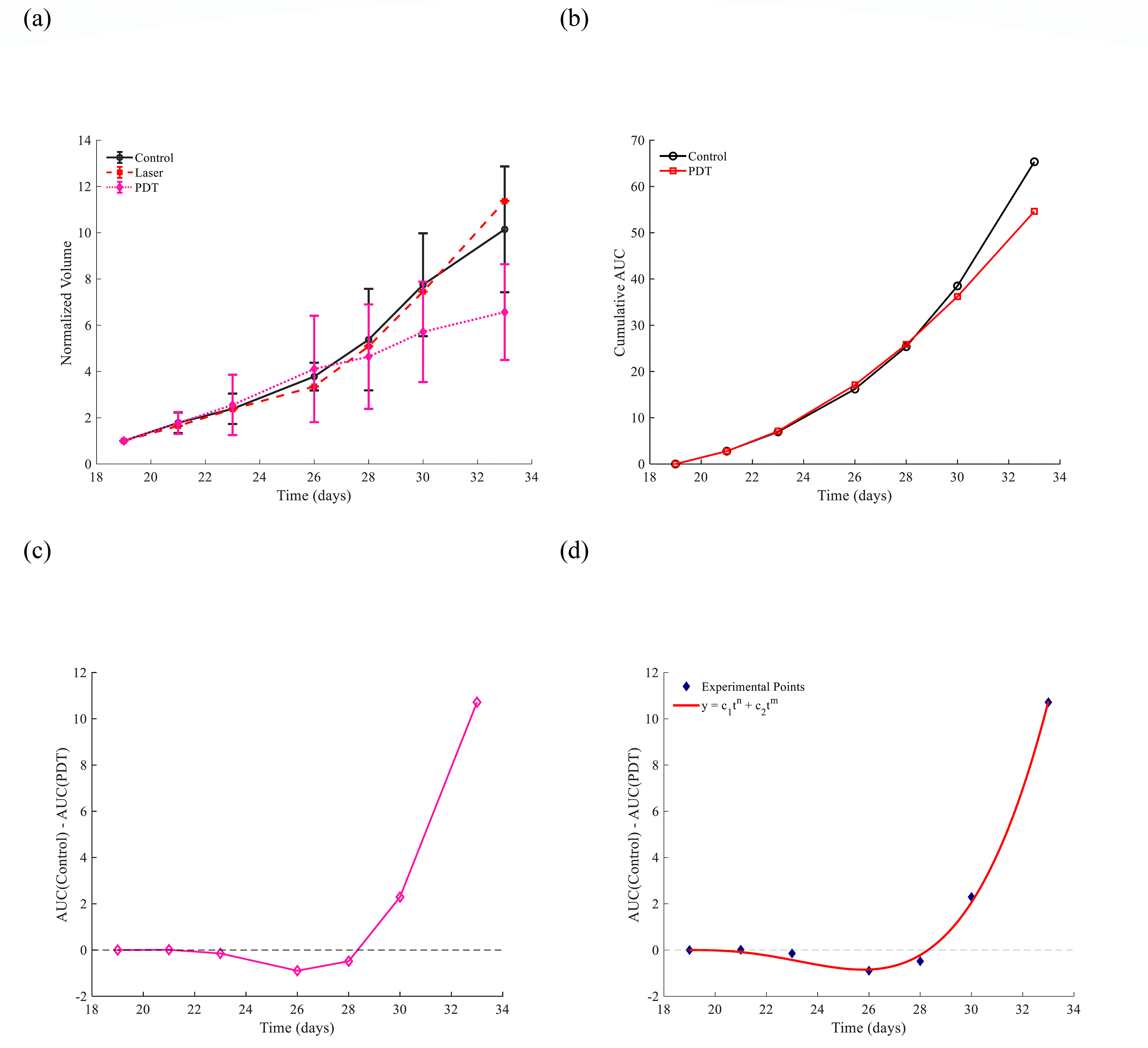
Figure 4. (a) Normalized tumor volume as a function of time for the Control, Laser-only, and PDT groups. (b) Cumulative tumor growth trajectories obtained using the AUC metric for the Control and PDT groups. (c) Difference between the cumulative trajectories (ΔAUC), illustrating the transition from an initial adverse response to a long-term therapeutic benefit after PDT. (d) Fitting of the ΔAUC data using the proposed mathematical model (Equation 46). Underlying data and MATLAB code are available in Zenodo.54
Therefore, PDT provides an ideal example for evaluating the accuracy of the proposed mathematical modeling framework for therapeutic approaches. By using the AUC metric, smooth cumulative trajectories are obtained for both the Control and PDT groups, as presented in Figure 4b. The difference between these trajectories is defined as:
(55)
and is presented in
Figure 4c.
The data presented in Figure 4c was fitted to Equation (46) and the fitting coefficients resulted in:
,
,
and
. The R-squared coefficient of the fitting resulted in
The early phase of the therapeutic process is described by the relationship
indicative a negative effect (i.e., an increase in the tumor volume) due to swelling as a result of the PDT process.55 However, the long term behavior is beneficial since
. The transition point is 9.31 days after the initiation of the PDT therapy, i.e. day 28.31. In addition, the stationary point (the minimum in the adverse-to-beneficial scenario) occurs at approximately 6.8 days after the starting point of the PDT therapy (i.e., day 25.31).
3.5 Modelling tranilast and doxorubicin treatments
As described in Section 2.4, the effects of tranilast and tranilast+doxorubicin treatment on breast cancer tumors in mice were evaluated. The normalized tumor volumes for the control, tranilast, and tranilast+doxorubicin groups are presented in Figure 5a. Tranilast was administered on day 7 (with day 1 defined as the day of tumor implantation in mice), while doxorubicin treatment was initiated on day 10 (see also reference [51]).While tranilast alone produces only a negligible reduction in tumor growth compared to the control group, the combined tranilast+doxorubicin treatment results in a pronounced suppression of tumor progression throughout the observation period. A clear separation between the control and tranilast+doxorubicin trajectories is observed, indicating a strong therapeutic response. Using the AUC metric, cumulative growth trajectories were calculated for the Control and Tranilast–Doxorubicin groups, as shown in Figure 5b. The difference between these trajectories is defined as:
(56)
and is presented in
Figure 5c. The data presented in
Figure 5c was fitted to
Equation (46) as below:
(57)
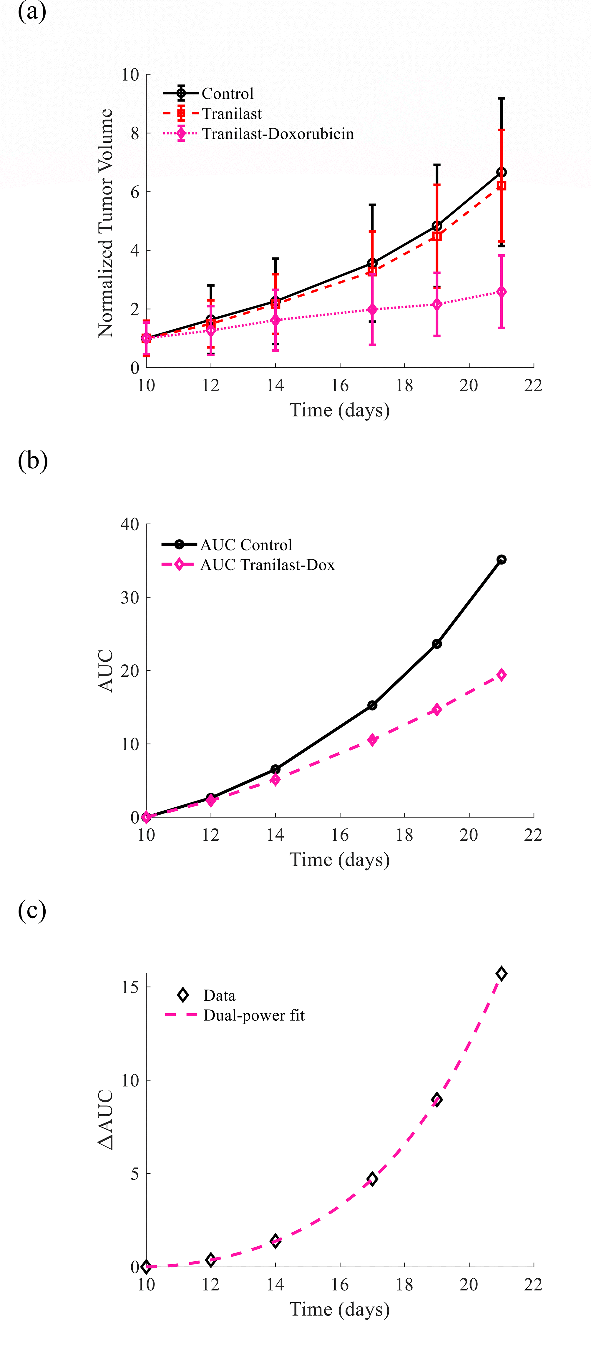
Figure 5. (a) Normalized tumor volumes for Control, Tranilast, and Tranilast–Doxorubicin groups, showing limited effect of Tranilast alone and strong tumor growth suppression under the combined treatment. (b) Cumulative AUC trajectories and their difference further highlight the enhanced therapeutic response of the combination therapy compared with Control. (c) Fitting of the ΔAUC data using the proposed mathematical model (Equation 57).
The R-squared coefficient in this case resulted in
In this case, a clear positive effect of the tranilast–doxorubicin treatment is observed, which is mathematically described by
Equation (57).
4. Discussion
The usefulness of mathematical oncology depends strongly on the quality and stability of the data used. Standard tumor monitoring relies on discrete volume measurements over time, which often appear irregular because of measurement noise (such as small variations in caliper placement or tumor shape estimation) and short-term biological fluctuations. In this work, it was shown that using a cumulative (integrated) measure of tumor burden helps reduce these fluctuations. The integration process naturally smooths the data, acting like a filter that reduces random noise effects over time. As a result, while measurement variability is still present at each time point, its relative impact becomes smaller when data are accumulated. This leads to smoother and more stable tumor growth curves that better reflect the true long-term behavior of the tumor compared to raw measurements. Furthermore, this framework addresses a major limitation in traditional cancer studies, which is the use of only the final tumor volume
to evaluate treatment effectiveness. From a dynamical systems point of view, endpoint measurements are incomplete because they ignore the full-time evolution of the tumor. As a result, very different growth or treatment responses can lead to the same final volume, even if their behavior during the treatment period is completely different. By reformulating the problem in terms of a “regularity–energy” landscape inspired by classical mechanics, the framework accounts for the full trajectory of tumor evolution. It introduces a regularization term (α) that penalizes large or unstable changes in volume over time. Within linear coupling assumptions, it is then shown that the true treatment-induced deviation in the trajectory (ΔS) is directly proportional to AUC, linking the overall disease progression to a single integrated measure rather than just the final state.
The second-order Euler–Cauchy formulation adds the necessary flexibility to describe complex biological responses that occur across different regimes, while still preserving scale invariance. In clinical situations, therapies such as PDT can cause immediate local inflammation or edema, which temporarily increases the measured tumor volume and can resemble disease progression. A single power-law model cannot capture this behavior. More specifically, consider a treatment-response variable of the form
where
,
,
, and
. Since
it follows that:
(58)
Therefore, the sign of
remains constant throughout the observation interval. If
, then
for all
, whereas if
, then
for all
. Consequently, no transition point
satisfying
can exist.
Thus, a single power-law mode is mathematically incapable of describing treatment-response reversals, such as an initially adverse response followed by long-term therapeutic benefit. To represent such biologically relevant transitions, at least two competing scale-invariant modes are required. The simplest formulation satisfying this requirement is given by
Equation (46) with
In this case, the lower-order mode dominates the early response, whereas the higher-order mode governs the long-term behavior. Their competition naturally generates a zero-crossing point corresponding to a transition from an initially adverse response to a later beneficial response, or vice versa. Importantly, the second-order Euler–Cauchy equation is the lowest-order scale-invariant differential equation whose general solution contains exactly two independent power-law modes. Therefore, the Euler–Cauchy formulation adopted in the present work is not merely a curve-fitting choice, but the minimal scale-invariant dynamical framework capable of describing treatment-response reversals. The practical usefulness of this framework is supported by its accurate reproduction of both the PDT and the Tranilast-Doxorubicin treatment trajectories, demonstrating its ability to capture distinct therapeutic-response patterns within a unified mathematical formulation.
Although the proposed AUC-based framework provides a new perspective for analyzing treatment-response dynamics, some limitations should be acknowledged. First, the datasets analyzed in this study involve relatively small numbers of biological replicates, as commonly encountered in preliminary in vivo oncology studies. Therefore, while the Euler–Cauchy formulation demonstrates excellent agreement with the observed cumulative response trajectories, the obtained fitting parameters should be interpreted primarily as descriptive of the investigated datasets rather than as definitive predictors. Future studies with larger cohorts and independent experiments will be important to further evaluate parameter robustness and generalizability.
Second, the present analysis focuses on demonstrating the ability of the framework to describe treatment-induced changes in cumulative tumor burden within the experimentally accessible time window. The model is not intended to reproduce absolute tumor growth kinetics or saturation behavior, as in conventional growth models, since the experiments were terminated at predefined ethical endpoints before the late-stage saturation phase was reached. Future validation using independent treatment-response datasets will be valuable to assess whether parameters derived from early cumulative dynamics can reliably characterize subsequent responses.
Third, the Euler–Cauchy formulation is based on the assumption that scale-invariant behavior and weakly perturbed dynamics can provide a meaningful approximation of treatment-response evolution. Although these assumptions are supported by the observed experimental trends, biological systems may involve nonlinear interactions, time-dependent effects, immune responses, and microenvironmental changes that cannot be fully captured by the current formulation. Future extensions incorporating nonlinear and time-dependent scaling approaches may improve applicability to more complex therapeutic scenarios.
Finally, although AUC has been widely used as a cumulative measure in pharmacology and oncology, the contribution of the present framework lies in treating cumulative tumor burden as a dynamical variable coupled with mathematical response modeling rather than as a simple endpoint metric. Further integration with pharmacokinetic/pharmacodynamic (PK/PD) models and validation across different tumor types and treatment modalities will help determine its broader applicability.
From a broader perspective, future developments should extend the framework toward heterogeneous and mechanistically informed tumor models by incorporating nonlinear interactions, stochastic effects, immune components, and PK/PD relationships. Large-scale validation using independent datasets across multiple cancer types and therapeutic modalities will ultimately be required to determine whether the proposed approach can contribute to personalized treatment-response modeling and clinical decision support. The proposed approach for the evaluation of a treatment response on solid tumors is presented in Figure 6. The key conceptual advances of the proposed cumulative dynamics framework for quantitative tumor treatment-response assessment are also highlighted in
Table 1.
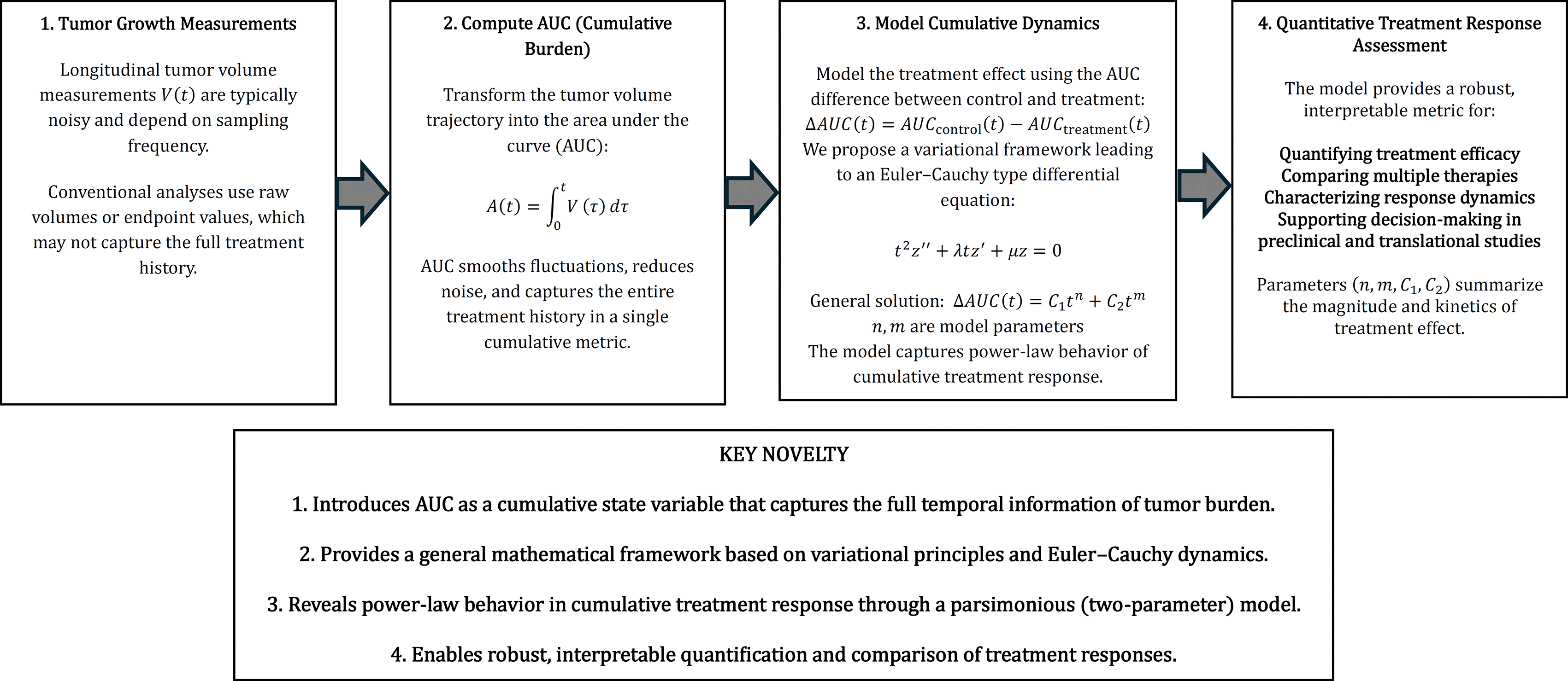
Figure 6. The proposed engineering-based procedure for the quantitively evaluation of the treatment response.
Table 1. Comparison between conventional tumor treatment-response assessment and the proposed cumulative dynamics framework.
|
Concept | Conventional view | This work |
|---|
| Primary variable | Tumor volume (V(t)) | Cumulative tumor burden
|
| Treatment-response metric | AUC as a retrospective summary statistic | AUC as the terminal value of a continuous cumulative dynamic process |
| Dynamic model | Single-phase empirical tumor-growth models | Scale-invariant Euler–Cauchy model describing multiphase therapeutic response |
| Medical Engineering contribution | Descriptive analysis of tumor growth | Medical engineering framework for quantitative longitudinal treatment-response assessment |
Ethics and consent
All animal experimental procedures were approved by the Cyprus Veterinary Services, the national authority responsible for monitoring and regulating animal research in Cyprus (license numbers CY/EXP/PR.L09/2025 and CY/EXP/PR.L2/2025). All experiments were conducted in accordance with the relevant national regulations and institutional guidelines for the care and use of laboratory animals.
This study did not involve human participants, human data, or human tissue samples; therefore, ethical approval and informed consent for human participation were not required.
Data availability statement
The appendices (Appendices A-D), containing the detailed mathematical derivations and supporting analyses referenced in the manuscript, are publicly available at Zenodo: https://zenodo.org/records/23033019.
Underlying data
Repository: Zenodo. DOI: 10.5281/zenodo.22068101.54
This project contains the following underlying data:
LASER-PDT_data.xlsx: Normalized tumour volume data as a function of time for the Control, Laser-only and PDT groups
LASER-PDT_data.xlsx: Area-under-the-curve (AUC) values calculated from the tumour growth data for the Control and PDT groups.
LASER-PDT_data.xlsx: Observed ΔAUC values and corresponding fitted ΔAUC values used for model validation and comparison with analytical predictions.
DATA_DESCRIPTION.txt: Description of all datasets, variables and data sources.
Plot4 a.m: MATLAB code used to create Figure 4a.
AUCdiff.m: MATLAB code used to create
Figures 4b-c.
fitDeltaAUC.m: MATLAB code used to fit Equation (46) to the experimental ΔAUC data and reproduce the results reported in the manuscript.
Data and code are available under the terms of the Creative Commons Attribution 4.0 International License (CC BY 4.0).
Extended data
No extended data are associated with this article.









