Introduction
Over the last seven decades, global fish production has increased along with the simultaneously increase in fish demand (2.4% increase rate per year between 1961 and 2017) and it is estimated to have reached 178.5 million tonnes in 2018 (FAO, 2020). Modern aquaculture has been constantly growing since it started around 1950 and, in the period between 2001 and 2018, it experienced a growth of 5.3% per year on average at a global scale (FAO, 2020). Today, aquaculture accounts for 46% of total fish production and 52% of fish for human consumption and its role is likely to increase further in the near future (FAO, 2020). In 2018, aquaculture production in EU Member States reached 1.2 million tonnes for an economic value of 4.1 billion Euros; it is mainly concentrated in four countries (Spain, France, Italy and Greece) that account for 69% of the total EU production volume (STECF, 2021). EU aquaculture production is dominated in terms of volume by shellfish with 56% of the total production, while freshwater and marine finfish production have a similar contribution: 21% and 23% respectively. EU aquaculture production is also highly selective in terms of reared species, with only nine species accounting for 90% in terms of weight (STECF, 2021).
Rainbow trout, Oncorhynchus mykiss, dominates EU freshwater aquaculture production, accounting for 53% in terms of volume and 56% in terms of economic value with the first three producers, Denmark, Italy and France, accounting for 67% of total EU volume for this species (STECF, 2021). In Italy, there is a long tradition of fish farming and rainbow trout represents the most farmed fish species, accounting for 27% of total Italian production from aquaculture (STECF, 2021). Rainbow trout farming is mainly located in the Northern part of the country (Fabris, 2012), which is characterized by a mountainous landscape that provides a suitable habitat for rainbow trout in terms of both cold/mild temperatures and well-oxygenated water (Sidoruk, 2019; Woynarovich et al., 2011).
Between 2008 and 2018, the production of rainbow trout in Europe decreased from 204,000 to 187,000 tonnes while, on the other hand, at a global level, production of rainbow trout rose from 518,000 to 848,000 tonnes. As a consequence, EU countries, have depended more and more on imports from other countries, especially from Asia, for domestic consumption of rainbow trout as well as other fish species (FAO, 2020; STECF, 2021). In order to reverse this trend, the European Commission (EC) has allocated economic resources to enhance aquaculture production in Europe. However, the increase in production of the aquaculture sector must be obtained within the framework of environmental sustainability, which prescribes a reduction of possible harmful effects on the surrounding environment of aquaculture practices (Bartoli et al., 2007; Ruiz-Zarzuela et al., 2009) to produce the same amount of fish, following the principle of Ecological Intensification (EI - Aubin et al., 2019).
The precision fish farming (PFF) approach represents a possible way to achieve the goal of EI. PFF aims to support fish farmers in decision making in order to improve both animal welfare and productivity by increasing accuracy, precision and repeatability in farming operations (Føre et al., 2018). This approach takes advantage of recent technological innovations in real-time detection of environmental variables and fish physiological response, and in the application of predictive models. Therefore, PFF will lead to the development of a new generation of dynamic models for predicting “animal variables”, based on sets of control variables, e.g. fish density and feed supply, and external forcing functions, e.g. water temperature and dissolved oxygen concentration. Fish weight is among the most important animal variable for fish farmers. There are several mathematical models for the simulation of weight growth of a rainbow trout population (Carlson et al., 2020; Clark et al., 2011; Deslauriers et al., 2017; Hayes et al., 2000; McCormick & High, 2020; Serchuk et al., 1980). However, these models have been applied to wild stocks for several purposes, e.g. habitat suitability and impacts of climate change, and they do not seem to be suitable for the aquaculture sector. For example, Fish bioenergetics 4.0 (Blair et al., 2013; Deslauriers et al., 2017) does not allow the combined simulation of weight and of optimal feed demand with time. In addition, population dynamics are considered to be due only to the age structure of the cohort and not due to phenotype differences. A model simulating the dynamics of weight distribution of farmed rainbow trout could provide useful information to fish farmers, such as: feed rations and liquid oxygen to be delivered, time to harvest and potential revenues.
The goals of this work were:
1. To develop an individual-based model for population dynamics (IBM-PD) of rainbow trout.
2. To test the model against a comprehensive data set, collected using a non-invasive monitoring system, i.e. Biomass Daily.
3. To show how model predictions could improve feeding.
Methods
Case study and monitoring strategy
The PFF approach was tested at a rainbow trout (O. mykiss) farm located in Preore (Trento - TN) in Northern Italy. The company is a family-run enterprise associated to the ASTRO Consortium. ASTRO has developed standardized protocols covering several key aspects of farm management: from feeding and water quality standards to quality of final products in terms of chemical composition of their flesh. The compliance with these standards is certified by a Protected Geographical Indication (PGI) label (Royer et al., 2021). The farm consisted of seven concrete raceways 200m long, 8m wide and 0.8m deep. These raceways were covered by a protection net in order to avoid predation by piscivorous birds. Water flowing through these raceways was withdrawn from the Sarca River and returned back to the same river.
The temporal evolution of weight distribution was monitored using Biomass Daily, (BD, Vaki), a non-invasive device, based on infrared technology. An individual fish size is determined starting from an infrared signal, detected anytime a specimen crosses a square frame. Observations are cumulated to track the temporal evolution of the distribution of weights. This system was previously deployed in cages of Atlantic salmon (Føre et al., 2016; Riveros, 2016); this was the first application to rainbow trout. Observations performed by BD are stored online and can be easily downloaded and post-processed for estimating daily statistics, such as mean and standard deviation of weight. The device was deployed in several in situ surveys carried out during the H2020 project Green Aquaculture Intensification (GAIN), in order to test it on a wide size range. During two surveys, i.e. August - September 2019 and July - November 2020, other field data were collected, namely: water temperature, daily feed ration, feed composition in terms of carbohydrates, lipids and proteins content. Hourly values of water temperature were collected during the two monitoring campaigns by a couple of identical multiparametric probes EXO2, commercialized by YSI, deployed at the inlet and at the outlet of the investigated raceway.
Individual-based model for population dynamics (IBM-PD)
The population dynamics was modelled using Equation 1 and Equation 2.
in which in which N(t) represents the number of individuals at time t and B(t) the total biomass at time t. The two parameters in Equation 1 represent a background mortality rate, mN, and the additional mortality rate associated to the outbreak of diseases, mv. Indeed, rainbow trout farming is commonly affected by outbreaks of several species of pathogens due to intensive production (Woynarovich et al., 2011). The total biomass was obtained by summing the weight wt,N of individuals surviving up to time t: these were estimated using the bioenergetic model described in the next section.
Individual growth model
The population dynamic was simulated excluding any interaction among individuals. Therefore, each individual weight followed its own trajectory of growth, based on its specific parameterization and initial condition. The simulated individuals can be either singular individual or be representative of a certain group, the so-called super-individuals, characterized by the same parametrization. Individual weights were simulated using the bioenergetic model presented in Equation 3 (Brigolin et al., 2010; Brigolin et al., 2014; Ursin, 1967). Model parameters are given in Table 2.
Equation 3 states an energy budget, in which w represents wet weight, A the net anabolism, depending on the energy feed content, C is the fasting catabolism, which quantifies the energy losses of a fasting individual, related to the respiration rate. Finally, εT is the energy content of the somatic tissue. Table 1 presents the functional expressions (Equation 4 – Equation 10) used to quantify each component of the energy budget of the bioenergetic model.
Table 1. List of functional expressions used to specify the growth model of rainbow trout.
| | 4 |
| | 5 |
| | 6 |
| | 7 |
| | 8 |
| | 9 |
| | 10 |
Table 2. List of the parameters used in the bioenergetic model of rainbow trout.
| Parameter | Description | Value | Unit | Source |
|---|
| Imax | Maximum ingestion rate | 1.831 | | Estimated on feeding table of Aller Aqua |
| α | Feeding catabolism coefficient | 0.58 | - | Calibrated in this work |
| βp | Assimilation coefficient for protein | 0.93 | - | Dalsgaard & Pedersen, 2011 |
| βl | Assimilation coefficient for lipid | 0.94 | - | Dalsgaard & Pedersen, 2011 |
| βc | Assimilation coefficient for carbohydrate | 0.67 | - | Dalsgaard & Pedersen, 2011 |
| εp | Energy content of protein | 23.6 | | Brett & Groves, 1979 |
| εl | Energy content of lipid | 36.2 | | Brett & Groves, 1979 |
| εc | Energy content of carbohydrate | 17.2 | | Brett & Groves, 1979 |
| εO2 | Energy consumed by the respiration of 1g of oxygen | 13.6 | | Brafield & Solomon, 1972 |
| εT | Energy content of 1g of somatic tissue | 5.763 | | van Poorten & Walters, 2010 |
| pk | Temperature coefficient for the fasting catabolism | 0.07 | °C–1 | Royer et al., 2021 |
| k0 | Fasting catabolism at 0°C | 8.5*10–4 | | Royer et al., 2021 |
| m | Weight exponent for the anabolism | 0.67 | - | From & Rasmussen, 2017 |
| b | Shape coefficient of the function H(Tw) | 0.2172 | - | Estimated on feeding table of Aller Aqua |
| n | Weight exponent for the catabolism | 0.8 | - | From & Rasmussen, 2017 |
| Tm | Maximum lethal temperature for O. mykiss | 25 | °C | Raleigh et al., 1984 |
| To | Optimal temperature for O.mykiss | 16 | °C | Raleigh et al., 1984;
Woynarovich et al., 2011 |
| Tlf | Lowest feeding temperature for O. mykiss | 2 | °C | Woynarovich et al., 2011 |
The individual model estimates the energy input based on feed daily ration, Iration, taking into account the digestibility and energy content of carbohydrates, lipids and proteins. Fish maximum ingestion was assumed to be proportional to fish size and temperature: this was taken as the energy intake if the fish ration exceeded this value. Ingestion was assumed to stop below a threshold temperature, named lowest feeding temperature, Tlf.
Three parameters affecting the anabolic component were estimated in this study, namely Imax, b and α. The first parameter represents the maximum daily feed ration at the optimal temperature, the second relates the daily ration to water temperature, through the function H(Tw). The parameter α quantifies energy costs associated to Specific Dynamic Action (SDA), to fish digestion, to assimilation and to swimming costs. The estimation strategy adopted for these parameters is presented below.
The performance of the individual growth model was evaluated using as Goodness of Fit Index (GoF) the root mean square error (RMSE). In addition, a Taylor diagram was used to evaluate this comparison between mean weights simulated by the model and mean weights estimated from daily distributions estimated using BD. The daily averages estimated using BD were also qualitatively compared with mean weights from routinely direct sampling performed by the trout farmer. The farmer mean weight was determined on the basis of different sample sizes, namely 50 individuals in 2019 and 200 in 2020.
The predictive capability of the IBM-PD was assessed based on the mean and the standard deviation of the fish weight distributions. The GoF indices were RMSE and R2 between the mean weights predicted by the model and mean weights estimated from observations collected by BD. For the standard deviation, the agreement was evaluated according to RMSE. Initial weights were assumed to be normally distributed and were determined by random extraction from normal distribution of the observations performed by BD. In addition, the weight structure of the population of rainbow trout within the raceway was simulated assuming that inter-individual physiological differences, due to diverse phenotypes, could be accounted for by slightly different values of the set of physiological parameters with respect to the mean individual. Specifically, two parameters were considered to change from individual to individual, namely the feeding catabolism coefficient, α, and the fasting catabolism at 0°C, k0. Each individual was characterized by a value for the parameter α that was randomly extracted from a normal distribution having a mean and standard deviation equal to those estimated previously during the calibration phase. Analogously, values for the parameter k0 were randomly extracted from a normal distribution having a mean and standard deviation equal to those presented in Royer et al. (2021).
Parameters estimation
The two parameters of Equation 1 were estimated by minimizing the following goal function Γ (Equation 11):
in which, Nobserved,t represents the number of fish observed at time t, while Npredicted,t corresponds to the number of individuals predicted according to Equation 1 at the same timestep.
Parameters Imax and b were estimated from the feeding table of Aller Artic SF, commercialized by Aller Aqua, which provides the feed ration as percentages of fish weight, at different temperatures for several classes of fish weights. Feeding rations were converted into energy, based on their composition in terms of proteins, lipids and carbohydrates and mean energy content of these macromolecules. The parameters Imax and b were determined by fitting the feeding table data using Equation 5 and Equation 6 of Table 1. A non-weighted least squares goal function was used for each class of fish weight.
Then, in order to describe average feed intake by an average individual in a whole rearing cycle, the mean was applied to best fitting estimates for every parameter, thus obtaining the two values presented in Table 2. In addition, standard deviation of these parameters was estimated in order to also consider the variability of these parameters according to each class of fish size.
The parameter α was estimated by calibrating the individual growth model against mean weights estimated from daily distribution of fish weights estimated using BD. The calibration of the model was performed by minimizing the goal function Θ (Equation 12).
In which: wobs,i represents the observed mean weight, while corresponds to the weight predicted by the model at day i. In order to estimate the expected value of the parameter α as well as its standard deviation, a procedure based on the Monte Carlo method (Royer et al., 2021) was applied. This method prescribes to calibrate (Equation 12) on a set of synthetic time series which are considered to be consistent with the observations from a statistical point of view. The synthetic data sets were created assuming that observations were time-independent and that weights were normally distributed. A set of 100 synthetic time series (Royer et al., 2021) was generated by random extraction from the daily distributions of weight. The calibration was repeated for each time series, thus, providing an empirical distribution of the α parameter.
The model and calibration algorithms were coded in R.
Feeding ration based on fish weight distribution
The daily feed ration is usually estimated based on: 1) feeding tables and FCR given by feed producers, 2) fish average weight, estimated by direct sampling approximately once a month in raceway trout farms, and 3) fish number. Most companies use specific software for this purpose, such as Fishmaker or Aquanetix. However, the relationship between fish maximum intake, Equation 5, and weight is not linear: therefore, feed rations estimated on the basis of fish size distribution using the following equation:
could be more accurate than those obtained by multiplying the average weight by the fish number.
This issue was explored by simulating a whole grow-out cycle lasting one year for a population of 5000 super-individuals (Brigolin et al., 2014), starting from a mean weight of 20g. The water temperature input to force the model was recorded at the trout farm from April 2020 to April 2021.
Ethical considerations
Ethical approval was obtained for the overarching Horizon 2020 GAIN Project. Ethical issues were summarized in project deliverables, that were presented and accepted by REA. Furthermore, the part of the study described in this paper did not deal with manipulation of animals or testing of fish feed, but only non-invasive monitoring systems. Thus, ethical approval for this study was not required.
Results
Individual model
From the interpolation of the feeding table, Imax resulted to be equal to 1831 with a standard deviation of 180 ; while b was equal to 0.2172 with a standard deviation of 0.0009.
Figure 1 shows the comparison of the estimated optimal feed ration, Iopt, derived from Equation 5 and presented in the feeding table. The black lines correspond to the estimated mean optimal feeding ration (solid line) simulated by this Equation with dashed lines representing the standard deviation around the mean value of the parameters Imax and b. The points in this graph represent the optimal feeding rations according to the analysed feeding table; in particular, each colour is representative of a different class of fish size.
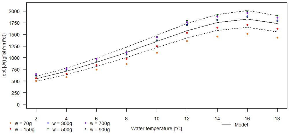
Figure 1. Comparison of optimal rations between model and feeding table as functions of water temperature.
Solid black line: estimated mean optimal ration. Dashed black lines: standard deviation around mean optimal ration. Points: feeding rations for fish size classes: 40g – 100g (orange); 100g – 200g (red); 200g – 400g (blue); 400g – 600g (dark green); 600g – 800g (purple); 800g – 1000g (dark grey).
The individual growth model was calibrated using the data set collected in the second survey, from 6 July to 3 November 2020, in which the average fish weight ranged from 300g to 600g; it was validated on the first data set (25 August 2019 – 3 September 2019), in which the average fish weight ranged from 1.3kg to 1.6kg.
The results of the calibration of the parameter α are shown in Figure 2, which presents a comparison between predicted weight by the individual growth model (black line), the average weight estimated from the observations collected by BD (red line) and mean weight observed by the farmer through samplings (dark green points). The grey line depicts the individual feed ration provided by the farmer along the period of simulation. As can be seen from this figure, qualitatively mean weights estimated from observations by BD and direct sampling were similar. The results of the calibration gave α = 0.579 ± 0.059. The GoF index was: RMSE of 33.37g, i.e. 8.72% of the average weight.
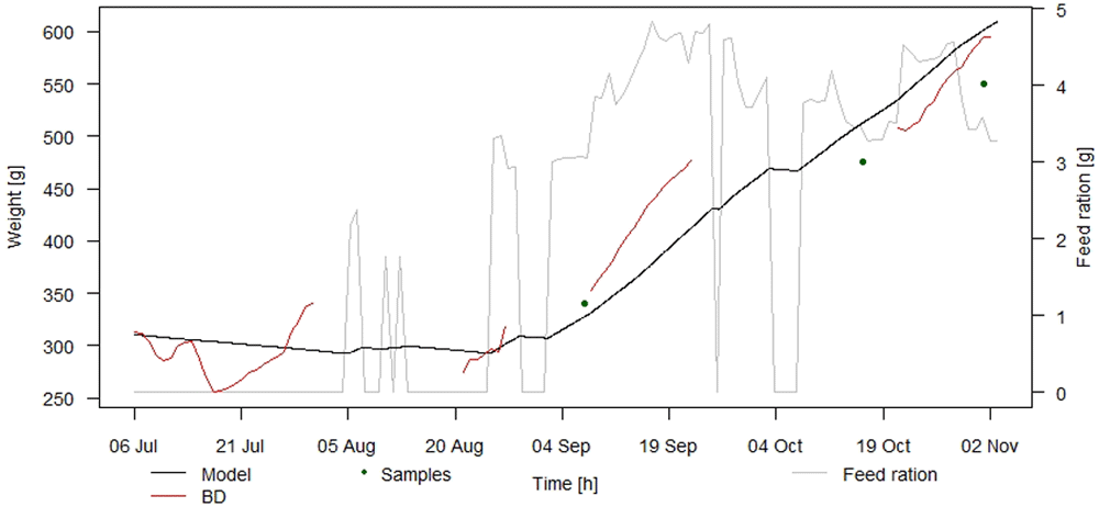
Figure 2. Calibration of the individual growth model of rainbow trout.
Black line: mean weight predicted by the mode. Red line: mean weight estimated by Biomass Daily (BD). Dots: mean weight by direct sampling. Grey line: feed ration.
The results of the validation of the individual bioenergetic model are presented in Figure 3. As can be seen, there was a good agreement between model predictions and observations. Indeed, the GoF index RMSE corresponded to 52.13g, i.e. 3.49% of the average weight.
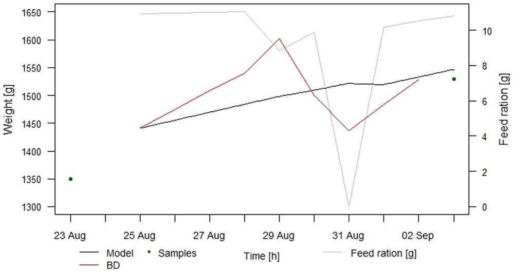
Figure 3. Validation of the individual growth model of rainbow trout. Black line: mean weight predicted by the model.
Red line: mean weight estimated by Biomass Daily (BD). Dots: mean weight by direct sampling. Grey line: feed ration.
Figure 4 shows the two Taylor diagrams obtained for the calibration (Figure 4a) and for the validation (Figure 4b) of the individual growth model. As can be seen from these figures, correlation between mean weight predicted by the model and the one estimated from observations by BD was equal to 0.95. On the other hand, the correlation in the validation result was quite low, being equal to 0.22.
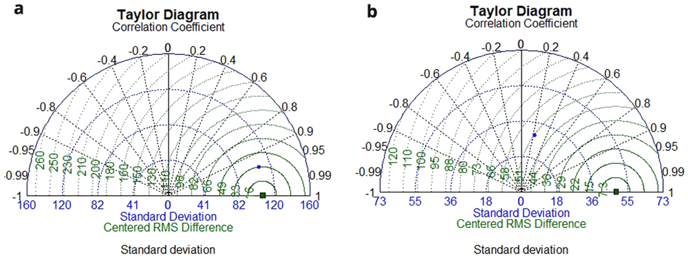
Figure 4.
Taylor diagrams for the calibration (a) and the validation (b) of the individual growth model.
Individual-based model for population dynamics (IBM-PD)
The IBM-PD was forced with the same data used for calibrating the model, simulating the whole population within the raceway, i.e. 39133 individuals. The results are presented in Figure 5, which shows the comparison between the mean and standard deviation of weight estimated using the model and those observed by BD. The R2 index for the mean weight was equal to 90.3%, while the RMSE corresponded to 30.75g, i.e. 7.95% of the average weight. For the standard deviation of weight, the RMSE was equal to 29.66g.
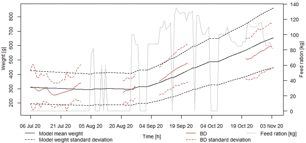
Figure 5. Comparison between the output of the population model and observations.
Black solid line: predicted mean weight; dashed black lines: standard deviation from the mean. Red solid line: mean weight observed by Biomass Daily (BD); dashed red lines: standard deviation from BD observations. Grey line: daily feed ration.
Figure 6 shows the comparison between the number of individuals alive in the raceway observed by the farmer (black points) with that predicted by the model at the same time t for the period from 6 July to 3 November 2020. Analogously to the individual growth model, Equation 1 was calibrated on real daily observations during the second monitoring survey and validated on the dataset of the first monitoring campaign. The pathogen Lactococcus Garvieae is endemic in trout farms located along the Sarca river, which are affected by the disease outbreak during the summer months. Outbreaks are prevented by vaccination, which is followed by a starvation period of about 6/7 weeks. The estimated natural mortality rate, mN, which minimizes the goal function Γ was equal to 0.0027, while the resulting additional mortality rate due to virus outbreak was equal to 0.0019. R2 was equal to 99.25%, while the RMSE resulted in 394 individuals, i.e. 1.29% of the average number of individuals within the raceway along time. In the validation window, the two GoF indices were R2 equal to 81.68% and RMSE was equal to 52 individuals, i.e. 0.46% of the average number of individuals within the raceway. In addition, in Figure 6, the grey line represents the total biomass estimated by the IBM-PD model at the same time and represents an example of the results provided by this model. As depicted by this curve, the IBM-PD model estimated a decrease in total biomass in the first two months because of both virus outbreak and starvation; however, after this period, total biomass increased because of the regular feeding regime.
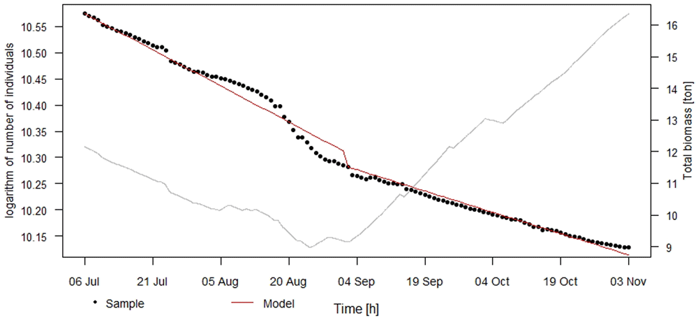
Figure 6. Comparison between number of fish observed by the farmer and predicted by the model along time.
Black points: natural logarithm of the number of individuals observed by the farmer; red line: natural logarithm of the number of individuals predicted by the model. Grey line: total biomass estimated by the model.
The overall feed demand estimated by the IBM-PD model for a rearing cycle lasting one year for an initial population of 5000 individuals was around 3414kg of feed. In the same simulation adopting the current practice for the estimation of daily feed ration based on optimal feed ration for the mean weight of the population and the number of individuals, the estimated amount of feed to deliver was around 3178kg. The resulting overall FCR was equal to 1.1. Hence, according to these results, current practice for the estimation of feed ration could lead to an overestimation of 1.02% compared to the overall feed demand estimated according to the IBM-PD model. Figure 7 shows the percentage of difference, black line, along the period of simulation. The grey lines in the background of this figure show the simulated mean weight of the population (solid grey line) along with the standard deviation of weight around the mean. As can be seen from this figure, the percentage of feed saved depends on time, from a minimum of around 0.6%, after one month of simulation and increasing up to 1.36% at the end of the simulation. In particular, it is worth highlighting that the percentage of saving increased with the increase in fish size distribution in terms of mean weight and its standard deviation.
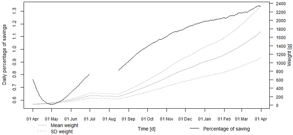
Figure 7. Percentage of difference in daily feed rations according to estimations by the individual-based model for population dynamics (IBM-PD) and to upscaling of mean individual weight.
Black line: percentage of saving. Grey lines, solid: mean weight of population; dashed: standard deviation of weight of population.
We proved that the adoption of the IBM- PD could address the issue of estimating feeding rations for a population; this analysis was also run for the rearing cycle observed under the second monitoring campaign in order to understand if the trout farmer could save part of the feed that he actually provided in that period. According to the results of this analysis, during the monitoring period, the trout farmer could have saved 2.23% of the total amount of feed provided, which means an economic saving of around 200€ in about two months of regular feeding regime and only for this raceway.
Discussion
In this work, an IBM-PD for rainbow trout, O. mykiss, was developed to supplement existing models (Blair et al., 2013; Deslauriers et al., 2017) that do not allow for the simulation of weight together with optimal feed rations as a function of time within the same simulation run. In addition, in these references, differences in weight growth of a population are only due to age structure of the population and not to phenotypical differences. The comparison between the predicted and observed mean weight and standard deviation was adequately predicted. The model requires the specification of 18 parameters and some assumptions on their range of variability. In this paragraph, limits of the growth model presented in this study are discussed, from issues related to the datasets used for the development of the individual growth model to comparison of the parameters estimated in this duty with literature findings.
The maximum feeding intake of rainbow trout was estimated in several previous studies (Deslauriers et al., 2017; Martens et al., 2014; Van Winkle et al., 1998). The model presented in Deslauriers et al. (2017) used four different equations to estimate the feed intake in relation to water temperature and fish size, but the equations (Equation 5 and Equation 6) proposed here require either the specification of a lower number of parameters or have a simpler formulation compared to Fish Bioenergetics 4.0. The same equations (Equation 5 and Equation 6) used in the growth model presented in this article were used by Brigolin et al. (2010), Brigolin et al. (2014). The value of the b parameter of Equation 6 found in this article was consistent with the values proposed in these articles, in which it ranged between 0.2 and 0.23. When converted into mass unit, for Imax a value of around 0.09 was estimated in this article, which is consistent with findings from Deslauriers et al. (2017).
The BD sensor was deployed for the first time in a trout farm, but as pointed out previously in presented figures (Figure 2 and Figure 3), mean weights estimated using this device showed daily fluctuations which, at times, were relevant, as the representativity of the sample is affected by its size, ranging from less than 10 observations in one day to around 4000 observations. However, the time series of average weight were consistent with the estimates obtained by direct sampling of 50 – 200 individuals. Agreement between these two measurements could not be quantitatively assessed because BD did not perform any observations for four days out of five, in which the trout farmer sampled the analysed population. Both datasets on which the individual growth model was calibrated and validated were characterized by periods in which observations by BD were not available for several reasons, such as malfunctioning of the sensor or loss of the internet connection. This affected the dataset used for validation, in which only those ten days considered were characterized by continuity in observations by BD. The results of the validation were good in terms of RMSE but, given the relatively large fluctuations of the BD data, the correlation between observed and predicted values, see the Taylor diagram in Figure 4b, is not very high. More robust results could have been obtained by extending the validation time window but, unfortunately, technical problems with the monitoring device prevented us from collecting more data.
The value of the feeding catabolism coefficient, α, found in this article was much higher than that reported in Elliott (1976) and Elliott & Persson (1978), i.e. 0.25 – 0.3. However, these studies were carried out in controlled laboratory conditions, which may not be representative of fish activity at large-scale, fully operational farms (Colt & Maynard, 2019). The Feed Conversion Ratio (FCR) estimated using the model in the calibration window was equal to 0.84, which is slightly lower than the interval proposed by the producer of the fish feed analysed, i.e. from 0.9 to 1.1, for the same class of fish size. On the other hand, the FCR estimated in the validation window was equal to 1.25, which is slightly greater than the interval suggested by the feed producer in the proposed feeding table, which ranges from 1 to 1.2 for the same fish size class. For a growth model that aims to simulate the grow-out phase of rainbow trout accurately for all fish size, then, the value of this parameter estimated in this study seems to be acceptable.
The IBM-PD was tested on two different sets of fish size: in particular, calibration was run for mean fish weight ranging between 300g and 600g, while validation took into consideration a mean fish size ranging between 1.3kg and 1.6kg. The predictive capability of the presented model can be compromised for fish weight outside of the considered ranges. However, while for fish size between 600g and 1kg rainbow trout growth along time can be reasonably estimated since trout experience the same granulometry of fish feed and belong to the adult phase, larger differences could be detected for fish weights ranging between 20g and 100g, because of the difference in fish stage, feed composition and feeding practice (Baruchelli, 2007).
The estimated background mortality rate, mN, was consistent with previous findings (Woynarovich et al., 2011).
Feed provisioning is currently based on the interpolation of the data provided in feeding tables and estimates of fish mean weight and number of individuals alive within the raceway. The model presented here could improve the estimation of daily feed ration, as it takes into account the non-linearity of the relationship between fish weight and appetite. Growth and feeding rations along time appear to be reasonably estimated since the FCR was equal to 1.1, which agrees with findings from literature (Woynarovich et al., 2011), feeding tables and trout farmer experience. The simulation also showed that the FCR changes with fish size, from 0.9 for 300g specimen to 1.2 for 1250g ones, in agreement with data published in EUMOFA (2021). The increase of the percentage of savings with fish size can be explained with the fact that the dispersion of the population distribution of weight increases along time, highlighting that taking into account the weight standard deviation as well allows a more accurate estimation of the feed ration.
Conclusions
In this work an IBM- PD was developed as a step toward the implementation of the PFF approach in rainbow trout farming. PFF makes use of real-time data from sensors as input for mathematical dynamic models in order to support fish farmers in their operations and promote the ecological transition of this sector. An individual growth model for this species was calibrated and validated using data collected by a non-invasive monitoring device, called Biomass Daily. The comparison between observations from this sensor and mean weight estimated by direct monthly samplings shows that the sensor provided reliable measurements, and its deployment, originally envisaged for salmon farming, can thus be extended to freshwater trout farming. The quantitative comparison between results of our model and different sets of observations carried out in this work suggests that population growth, in particular mean and standard deviation, is adequately predicted.
In this paper, we showed that the implementation of IBM-PD in trout farming can save a modest amount of fish feed and, hence, can increase the economic profitability of this activity.
For future works, it would be important to assess whether the adoption of the IBM-PD in relation to trout farming could be used for better estimating loads of nutrients released as well as oxygen demand (Royer et al., 2021). Analogously to what was observed with feed provisioning in rainbow trout farming, the implementation IBM-PD could also improve daily management of farms and support operators to comply with current European and national legislation, in terms of reduction of water quality discharged back into the environment, due to a reduction of wasted feed as demonstrated in this duty.
Data availability
Code and data are available from:.https://doi.org/10.5281/zenodo.6538136 (Bolzonella, 2022)
Five .zip folders are included:
feeding_table contains the code and the feeding table interpolated in this study;
calibration contains the code and the input files used for the calibration of the individual growth model of rainbow trout;
validation contains the code and the input files used for the validation of the individual growth model of rainbow trout;
Simulation_ideal_cycle contains the code and the input files for the simulation of the 1-year rearing cycle presented in this study;
Weight_pop_withmort_divided contains the simulated weight trajectories of the 5000 individuals in the 1-year rearing cycle presented in this study. Here, the code to combine these files is also present.
Data are available under the terms of the Creative Commons Attribution 4.0 International license (CC-BY 4.0).