Data processing workflow approach
The proposed data processing approach can be split into two steps as illustrated in Figure 1. The first step builds the Areas dataset, which host the necessary data variables from the pre-processed input data sources within a structured framework. A set of requirements are defined for the Areas dataset to ensure standardisation and proper documentation of the data variables. The first requirement prescribes that the data variables need to be indexed using standardised reference keys. These reference keys allow the data to be uniformly organised according to spatial, temporal, and technological specifications. The Nomenclature of Territorial Units for Statistics level 2 (NUTS 2) and NUTS level 0 are the two spatial reference keys used by the Areas dataset to structure data with a spatial dimension. The second requirement ensures the use of standardised units of measurements. The standardisation of units ensures uniformity, allowing the use of the dataset for modelling without additional unit conversions. The final requirement for building an Areas dataset is the documentation of the data variables in the dataset. The documentation entails providing the source of the data variables and a description of the unit.
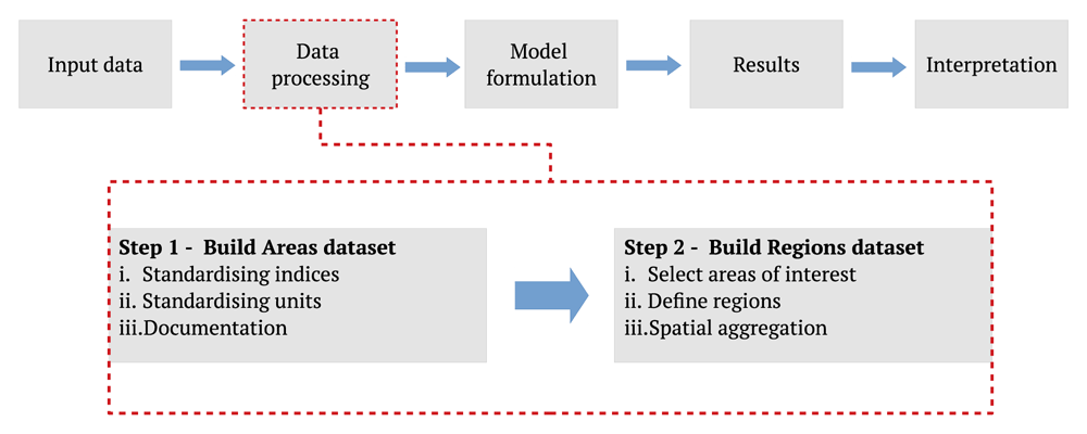
Figure 1. An illustrated description of the proposed data processing workflow of the energy system modelling process.
The energy system modelling process is based on the Openmod Philosophy laid out by Pfenninger et al. in 2.
Building a Regions dataset is the second step of the data processing process. The Regions dataset is constructed by first defining the areas of interest. The areas of interest could include all areas in the Areas dataset, or it could consist of a subset of areas. As the name of the dataset indicates, the Regions dataset allows for the grouping of areas into regions. The Regions dataset is described in more detail in Regions dataset.
Dataset framework. Two requirements were defined to guide the selection process of the dataset framework used as the skeleton for the Areas and the Regions dataset. The first requirement is that the dataset framework should be able to handle data with more than one reference key. The need for multiple reference keys handling capability allows data variables to be referenced according to spatial, temporal, or even technological indices. The second requirement is that the dataset framework must integrate well with existing open-source energy modelling software and scientific analysis software. As there is a multitude of these software15,27–30 written in the Python programming language31, the dataset framework should be a Python-based software. The xarray dataset object in the xarray toolkit32 was selected to build the datasets based on these two requirements.
There are additional benefits of using xarray to construct the datasets, as listed below:
the dataset can be exported as a unidata network common (nc) file format that can be compressed to lower file sizes which eases sharing of the datasets;
the dataset framework allows for documentation of the data variables.
As the datasets created can be stored and shared using a single file, they can also be made accessible using online archives such as Zenodo. Zenodo attaches Digital Object Identifiers (DOIs), which allows for the citation of the data. Hörsch et al.15 and Tröndle et al.16 both share different versions of their model on Zenodo using the nc file format.
Areas dataset. The Areas dataset spatial scope includes the EU 27 countries with the exclusion of Cyprus and Malta and the addition of Norway, Great Britain, and Switzerland. The data variables in the dataset can be sub-divided into two sets, the base variables and the derived variables. The base variables are used to determine the derived variables.
The Areas and the Regions datasets have a total of seven reference keys. There are two spatial reference keys, namely NUTS 0 and NUTS 2. Data variables using the NUTS 0 reference key apply at the national level, whereas the NUTS 2 level data are, for most countries, spatial administrative areas within the countries. There are four technology-specific reference keys: techs, fuels, techs hydro, and techs hydro subset. The techs and fuels reference keys reference the different technology types of the power plants variable. The techs hydro reference key is used to reference the technologies used to generate power from hydropower. The techs hydro subset dimension refers to a subset of the techs hydro reference key of hydropower technologies that have reservoirs to store water. The time reference key is used to index the time dimension of data variables. The time indices are the hourly intervals of a single representative year. The variables reference key, unit and sources are summarised in Table 1. Except for temperature and offshore wind capacity factor, the data variables in the Areas dataset are organised at the NUTS 2 spatial level. Therefore, the Areas dataset can be considered as a collection of data variables of 270 NUTS 2 areas.
Table 1. Summary of the data variables in the Areas dataset.
| Data variable | Base/Derived
variables | Reference key | Unit | Sources |
|---|
| NUTS 2 id | Base |
NUTS 2
| NA | 33 |
| Geometry | Base |
NUTS 2
| NA | 33 |
| Country code | Base |
NUTS 2
| NA | 33 |
| Temperature | Base |
time, NUTS 0
| Degrees Celsius | 20 |
| Population | Base |
NUTS 2
| people | 34 |
| Power plants | Base |
techs, fuels, NUTS 2
| MW | 35–37 |
| Hydropower plants dispatch | Base |
techs hydro, NUTS 2
| MW | 38 |
| Hydropower plants storage | Base |
techs hydro subset, NUTS 2
| MW, MWh | 38 |
| Rooftop solar PV area | Base |
NUTS 2
| km2 | 39–42 |
| Ground-mounted solar PV | Base |
NUTS 2
| km2 | 39–42 |
| Onshore wind area | Base |
NUTS 2
| km2 | 22,43,44 |
| Offshore wind area | Base |
NUTS 2
| km2 | 43,45 |
| Solar capacity factor | Base |
time, NUTS 2
| Per unit capacity | 20 |
| Wind capacity factor | Base |
time, NUTS 2
| Per unit capacity | 20 |
| Offshore wind capacity factor | Base |
time, NUTS 0
| Per unit capacity | 20 |
| Hydropower capacity factor | Base |
time, NUTS 2
| Per unit capacity | 46 |
| Power | Derived |
time, NUTS 2
| MW | 47 |
| Heat | Derived |
time, NUTS 2
| MW | 22 |
| Air-sourced capacity factor | Derived |
time, NUTS 2
| Per unit capacity | 20,22 |
Base variables
There are a set of base variables needed to establish the foundation of the dataset. The identification code (NUTS 2 id), the geometrical information (Geometry), and the country identification code (Country code) of the NUTS 2 areas are base variables taken from the Eurostat database33. The NUTS 2 geometry scale is 1:10 million. The ambient air temperature obtained from annual hourly historical weather data from the renewables.ninja platform20 is a base variable in the NUS T 2 area dataset. The weather data is only available at the country level, so the temperature data is given at NUTS 0 in the dataset. The population values in the NUTS 2 areas are extracted from the Global Human Settlement (GHS) population grid34. The population raster for the year 2015 was used. The population values within the geometry of the NUTS 2 area are summed, and the sum is the population value assigned to the NUTS 2 area. Other base variables describe the energy generation and storage technologies.
The power plants data variable gives the aggregated installed capacity of conventional power plants, solar photovoltaic (PV) installations, onshore and offshore wind installations associated with the NUTS 2 areas. Information on conventional power plants is from the conventional power plants dataset hosted on the OPSD platform34. Information on solar and onshore wind installations for NUTS 2 areas in Germany, Denmark, France, Poland, United Kingdom and Switzerland, were extracted from the OPSD renewable power plants dataset35. A power plant from the two datasets is associated with a NUTS 2 area when the power plants’ geometrical information places it within the geometrical boundaries of that NUTS 2 area. The power plants are grouped by the fuel and technology type and aggregated by their installed generating capacity in megawatts (MW). As the offshore wind installations are not within the geometries of the NUTS 2 areas, they are determined separately. The existing offshore wind installations were extracted from the European Marine Observation and Data Network (EMODnet) offshore wind farm database36. This database provides the location of each wind farm as a georeferenced point and references it to a country. The offshore wind farms were assigned to the closest NUTS 2 area of the country it was referenced too.
The dataset has three categories of hydropower technologies: run-of-river hydropower, reservoir-based hydropower and pumped storage hydropower obtained from the Joint Research Council (JRC) hydropower plants database38. The NUTS 2 areas were assigned the cumulative installed capacity of the different hydropower capacities. The reservoir-based and pumped storage hydropower plants’ cumulative storage capacity within the NUTS 2 areas was also calculated and added to the dataset. In the instances where the storage capacity was not given, it was assumed that the plant had a reservoir that can store the water needed to operate the plant at nominal capacity for six hours.
The availability of onshore wind and solar were assigned to the dataset as hourly capacity factor values extracted for each NUTS 2 area from renewables.ninja platform20. The capacity factors for offshore wind at the national level was taken from the same data platform. The country-wide daily inflow from 46 defines the capacity factor of the hydropower plants provides the historical daily inflow in 30 European countries between 2003 to 2012. The hydropower plants’ capacity factors were calculated by dividing the daily inflow values by the sum of installed hydropower capacity within the country.
The data variables that define the area available for renewable energy technologies are rooftop solar PV area, ground-mounted solar PV area, onshore wind area and offshore wind area. For the NUTS 2 areas in the EU-27 countries and the United Kingdom, the ENSPRESSO database was used to assign the data variables of rooftop and ground-mounted solar PV area39 and the data variables for onshore and offshore wind area43. The areas classified in the EU-wide low restrictions with 400 m setback distance scenario were selected to define the onshore wind areas. The onshore wind areas in NUTS2 areas of Switzerland were calculated from the wind energy potential areas raster provided by the swiss energy ministry44. The onshore wind areas in NUTS 2 areas in Norway were calculated from the wind energy potential areas raster of the hotmaps project22.
The areas classified within the EU-wide low restrictions with water depth 0 – 30 m and water depth 30 – 60 m scenario were selected from 43 to determine the offshore wind area. Except for the NUTS 2 areas in Norway, the portion of the offshore wind areas assigned to a NUTS 2 area is proportional to their share of their respective country’s total coastline. The NUTS 2 areas of Norway are assigned offshore wind areas according to their proximity to the offshore wind areas listed in the Norwegian offshore wind strategic environmental assessment report45.
The rooftop and ground-mounted solar PV areas in Switzerland and Norway were calculated using the Open Street Map building footprint data42 and literature values. For Switzerland, the rooftop solar PV area in a NUTS 2 area was proportional to their share of the total building footprint area in Switzerland multiplied by a total available rooftop area of 267 km2 and a rooftop suitability factor of 0.564 provided by Walch et al. in 40. For Norway, the rooftop solar PV area was calculated by multiplying the total building footprint area within the NUTS 2 areas with an rooftop area suitability factor of 0.49 calculated by Bódis et al. in 41. The ground-mounted solar PV area in Norway and Switzerland was calculated using the ratio of the ground-mounted solar PV area to the rooftop solar PV of Sweden and Austria, respectively. These ratios are 176:1 and 144:1, respectively.
Derived variables
Historical hourly electrical load profiles, at the country level, for European countries, are available on the European Network of Transmission System Operators (ENTSO-E) transparency platform47. For the reference year selected, hourly load profiles of the NUTS 2 areas are multiplied with the NUTS 2 areas population factor. The population factor of a NUTS 2 area is the share of the population in that area in relation to the population of NUTS 2 area respective country.
Using a bottom-up approach, the heat demand profiles Da,t are generated for each NUST 2 area a and time step t using the following equation:
The bottom-up approach classifies the heat demand in two end-use categories e and two sectors s. The end-use categories are space heating and domestic hot water heating. The sectors are the tertiary and domestic sector. Both end-use categories of each sector have a share factor σa,s,e and a normalised hourly profile da,s,e,t with time steps t. The share factor gives the percentage contribution of an end-use category of a sector to the total space and water heating demand. These share factors are country-specific and are obtained from the hotmaps repository22. The hotmaps repository does not provide share factor values for Norway and Switzerland22. Therefore, the share factors for Sweden and Luxemburg were used respectively instead. The normalised profiles are generated at the national level using generic profiles for space heating and water heating obtained from the hotmaps repository22. The generic profiles for space heating are country, season and temperature-dependent whereas, the generic profiles of hot water heating only vary according to the day of the week and the season. The normalised space heating profiles are defined using the temperature data in the dataset. NUTS 2 areas within the same country are assigned the same normalised space heating demand profile. The heat demand volume da for space heating and hot water heating is calculated from a rasterised map generated by the hotmaps project22. The map depicts the estimated final energy demand for space and water heating on each hectare for EU28, Norway, Iceland and Switzerland for 2015.
The temperature variables from the dataset are used to calculate the hourly efficiency factors of the heat pumps. The efficiency of the air-sourced heat pumps is calculated using the Carnot coefficient of performance (COP) equation, a maximum COP value of 3.2 and a room temperature of 21°C.
Regions dataset. Spatial resolution reduction is often used to reduce the computational demand of solving energy system optimisation problems. Depending on the research question or study focus, the data can be aggregated into regions to reduce the spatial resolution of the dataset. A common spatial resolution reduction method used by energy system modellers is to aggregate the spatial data according to political or administrative boundaries. European countries are classified according to multiple NUTS levels. The political regions method can thus group areas according to the NUTS level specified. For example, the spatial resolution of the data for Germany would reduce from 38 government regions of the NUTS 2 areas to the 16 states of NUTS 1. The spatial resolution could also be further reduced to a national level by aggregating the NUTS 2 area data to the NUTS 0 level. The number of NUTS areas at different levels is dependent on the European country. There are spatial resolution reduction methods that group areas according to the heterogeneity of spatial attributes of NUTS 2 areas. The max-p regions method for example, presented by Fleischer12, groups areas into regions that are similar in population; wind and solar resource potential; and pumped-hydro storage capacity. The max-p regions method uses the max-p-regions algorithm, introduced by Duque et al. in 48.
Once the regions are defined, the variables of the NUTS 2 areas are aggregated to have variables that represent the regions. The resulting spatially aggregated dataset, hereafter referred to as the Regions dataset, is used to store and organise the variables generated after data aggregation. In the Regions dataset, the NUTS 2 reference key is replaced by the Regions reference key. The Regions reference key is composed of the NUTS 2 reference keys of the NUTS 2 area within the regions created. The geometry of the NUTS 2 areas attributed to the same region are joined to form the geometry of the regions.
The capacity factors of wind and solar are multiplied by a weight value before they are summed. The weight value is the share of land area value of the NUTS 2 area in relation to the land area in the respective appointed region. For the capacity factor of offshore wind, the weight value is the share of the offshore area in the NUTS 2 area in relation to the appointed region. The capacity factors of hydropower are weighed according to the area of the NUTS 2 areas in the regions. All other variables do not represent mean values and are summed without weight factors.
Model formulation. There are some additional items needed in conjunction with a Regions dataset to formulate an energy system model. The first item is an energy system framework. There is a selection of open-source energy modelling frameworks that can be used. The selection of the framework depends on the focus of the study and the preference of the modeller. As the Regions database is generated using the python programming language, it can be integrated well into a python-based modelling framework.
Together with some additional items, the Regions dataset can then be used to formulate energy system models. One essential item is the techno-economic parameters. The techno-economic parameters will depend on the scenarios being investigated by the model. The scenarios also dictate certain assumptions used in the model.
Power and heat optimisation model development
The proposed data processing workflow, implemented in the EUropean Sustainable Energy System (EU-SES) modelling tool49, is used to build power and heat optimisation models to demonstrate the versatility of the data processing approach and the importance of spatial context in energy system modelling. The EU-SES tool uses the calliope framework27 to formulate the models. The scripts used to generate the datasets, models and the optimisation results of each model can be found on Zenodo50.
The first model is a multi-national model containing ten countries in the NUTS 2 area dataset named the GER NUTS0 model. These ten countries include Germany and nine countries that have a transmission connection with Germany. The NUTS 2 areas spatial data are aggregated according to national jurisdiction in the GER NUTS0 model. The second and third model reduces the spatial scope to include only Germany with no energy import or export from neighbouring countries. The difference between the second and third model is the spatial resolution reduction method used. The second model, named the GER NUTS1 model, are defined according to 16 administrative jurisdictions given by the NUTS 1 level. Whereas the regions in the third model, named the GER MAX-P model, are defined using the max-p regions method to generate nine regions. As illustrated in part a) of Figure 3, GER NUTS 1 model has more regions and therefore, the regions have, on average, a higher spatial resolution than the regions in the GER MAX-P model. The regions with the highest spatial resolution in the GER NUTS 1 model represent the city-states of Berlin, Hamburg and Bremen.
To investigate the effect of rooftop solar PV availability on the optimisation results of two models with the same spatial scope but with two different spatial resolutions, the GER NUTS1 and GER MAX-P model are optimised with and without the availability of rooftop solar PV areas.
The reference year selected to create the Areas dataset is 2010. The structure of the models is illustrated in Figure 2. The examples are modelled using the calliope modelling framework.
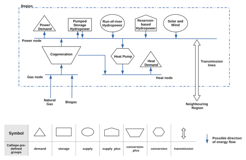
Figure 2. An illustrated description of the model created using the regions dataset and the calliope modelling framework.
The table in the figure indicates the predefined technology groups used to describe the different components in the model.
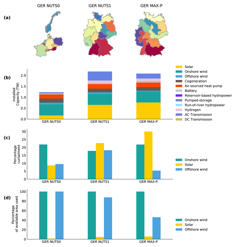
Figure 3.
The regions in the GER NUTS0 model, GER NUTS1 model and the GER Max-P model, are illustrated in a). The least-cost optimisation results of the three models for Germany are given in b), c) and d). Plot b) illustrates the optimised installed capacity of the technologies. The curtailment rate of solar PV, onshore and offshore wind generation is given in percentage value in c). Plot d) illustrates the optimised percentage of the available area utilised by solar, onshore and offshore wind installations.
The models all share several overarching scenario assumptions. The following key assumptions are made in this scenario:
• The cumulative CO2 equivalent emission of the optimised model is limited to 20 % of the 1990 CO2 equivalent emission of the countries in the model;
• The cumulative biogas available to the cogeneration plants is 420 PJ which was estimated to be a projected value for 2020 presented by Scarlat et al. in 51;
• All power plant capacities classified as biomass, gas and cogeneration in the Regions dataset are summed under the classification cogeneration;
• Power plants classified as nuclear, coal, oil, other, waste and geothermal in the Regions dataset are not available in the model;
• The storage level of all storage capacities is assumed to be full during the first and last instance of the optimisation;
• The hydropower power plants, existing installed wind and solar capacities must be adopted in the optimised model;
• All models have available only 50% of the ground-mounted area identified available for solar PV installations;
• The solar and onshore wind capacity density is assumed to be 170 MW/km2 and 5 MW/km2, respectively, adopted from Ruiz et al.23;
• Offshore wind installations have a capacity density of 5.36 MW/km2 adopted from Hundleby and Freeman52;
• Regions are considered ‘copper plates’, meaning that within the regions there are no constraints in energy transfer.
The power exchange between regions is possible and is constrained by the net transfer capacity and the efficiency of the power lines. There are two power transfer mediums in the model. The first is the high voltage alternative current (HVAC) transmission lines between regions that share a border. The HVAC has a minimum rated capacity of 2 GW and can be expanded by the model to a rated capacity of 8 gigawatts (GW). An HVAC transmission line capacity can be expanded at the cost of 400 €/MWkm adopted from Schlachtberger et al. in 53. The other power transfer mediums are direct current high voltage interconnectors installed between regions. The list of interconnectors and their respective rated transfer capacity is taken from the installed and planned DC links listed by Fleischer et al. in 12. Losses are not considered in the interconnectors and HVAC transmission lines.
The power and heat optimisation model’s objective function is to minimise the investment cost and dispatch cost of the model for one year and at a three-hour resolution. The optimisation models assume perfect foresight, and the power and heat demand is inelastic. A discount rate of 7% is assumed to calculate the annualised cost of the investments. The model uses techno-economic parameters projected for the year 2030, documented as Extended data54. The techno-economic parameters for the generation and storage technologies were adopted from values presented by Moles et al.55 and by Jülch56, respectively.