Introduction
Ever since the demonstration of the superior operation of an optical atomic clock1–3 with respect to microwave implementations people started wondering about a possible active clock implementation in form of a superradiant laser4–20. In analogy to the very successful hydrogen micro-maser technology21 such an active device in principle promises at least similar stability and accuracy at a reduced technical cost and fragility. Here an implementation based on a dilute gas of cold clock atoms within a high-Q optical cavity was predicted to be a very promising path to go5. As a particular example, model setups based on a beam of inverted ultracold atoms traversing an optical resonator22–24 were predicted to yield unprecedented stability and accuracy. However, as the operating optical wavelength (∼500 nm) is several orders of magnitude shorter than the typical maser lines (∼20 cm), the resulting technological challenges are similarly larger.
Already the construction of a suitable beam source is virtually equivalent to operating a continuous atom laser25,26 and thus poses a way more challenging task than its microwave analog. As the cavity mode volume is also way smaller the atoms have to be tightly confined before sending them through the resonator. Yet another problem is creating atomic inversion with minimal perturbation27. Despite intense efforts which recently lead to amazing technical advancements on guided atom beams28–31 and pulsed superradiant lasing32–39, a fully continuous operating device9,19 has not been realized.
In recent calculations it was pointed out that a high precision could already be achieved using a much hotter atomic ensemble with a sufficiently high intra-cavity density24,40–42. Here the sheer number of contributing atoms allows to cross the laser threshold inducing an efficient collective synchronization process towards a very narrow effective linewidth. This approach at least in principle requires significantly less components and would allow for a rather compact setup involving only a beam oven, an optical resonator and a pump laser to create inversion. The precise conditions for a concrete setup, however, cannot be reliably analytically predicted and thus require large scale numerical simulations24. Here we set up a framework for such simulations which can deal with realistically large atom numbers and velocities. This allows to identify the minimal operating conditions and study the influence of extra elements as velocity filters or guiding potentials.
Methods: Theoretical Model
We consider an ensemble of N two-level atoms with a transition frequency of ωa coupled to a single mode cavity with resonance frequency ωc, see Figure 1. The coherent dynamics of this system is governed by the Tavis Cummings Hamiltonian, which in the rotating frame of the atomic transition frequency ωa reads
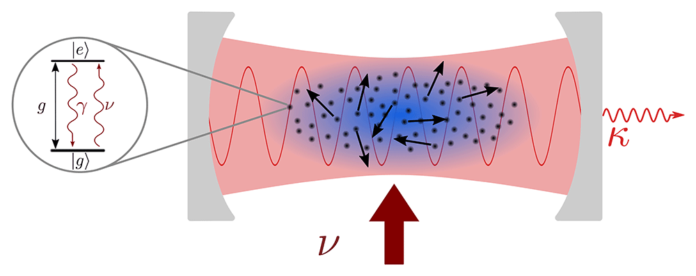
Figure 1. Schematic of the system.
Atoms are incoherently pumped with rate ν and couple to an optical cavity. The clusters move according to a Gaussian velocity distribution with standard deviation σv, which relates to a certain temperature T. This motion is included along the cavity axis with a position dependent coupling strength g. The atoms decay with the rate γ and the photons leak out of the cavity with a rate κ.
with the atomic transition operator of the j-th atom the cavity photon creation (annihilation) operator a† (a), and the cavity-atom detuning ∆ = ωc – ωa. Atoms at a position x along the cavity axis couple to the cavity according to the mode function g • f (x) = g • cos(2πx/λ), where g is the maximal cavity coupling strength and λ the wavelength of the cavity photons. The motion of the atoms is treated classically by an initial atomic velocity drawn from a Gaussian distribution with width σv corresponding to a temperature T. In the beginning we treat freely moving atoms, later on we investigate the influence of an external optical potential. In both cases the atomic motion is fully determined by the initial velocity and position.
Additional to the coherent dynamics we need to account for the dissipative processes, which are described by Liouvillian term ℒ[ρ] in the master equation for the system density matrix ρ
In the Born-Markov approximation the Liouvillian super-operator for a jump operator Ji with a corresponding rate Γi can be written in Lindblad form as
The considered dissipative processes are listed in Table 1, including cavity photon losses, individual spontaneous decay as well as incoherent pumping of the two-level atoms.
Table 1. Dissipative Processes.
The system features a damped cavity mode, atomic decay and an incoherent pump.
| i | ci | Γi | Description |
|---|
| 1 | a | κ | cavity photon losses |
| 2 | | γ | decay from |e〉j to |g〉j |
| 3 | | ν | excitation of the j-th atom |
As we want to simulate systems with up to one million atoms, we cannot solve the full master equation due to exponential scaling of the size of the Hilbert space with the particle number. To this end we employ a mean field approach for operator averages. For a non-explicitly time-dependent operator 𝒪 we can calculate the time-evolution of its expectation value as
with
where we inserted the master Equation (2) into Equation (4) and used the cyclic property of the trace. To truncate the set of equations we approximate higher order quantum correlations with the cumulant expansion method43,44.
The first order approximation (mean field) is sufficient to accurately describe our system (see Appendix), the corresponding set of equations is
where the last two equations exist for each atom from m = 1 to N. The number of equations in this approximation scales linearly with the atom number N. Still, to simulate a system with several hundred thousand atoms we need further approximations. To this end, we assume that groups of K atoms behave in a sufficiently identical way, such that we can describe them with the same equations. This means, we group atoms into clusters. For the set of equations in 6, this means that the index m now runs only from m = 1 to the number of clusters NCl, but the source term in Equation (6a) gets enhanced by the clustersize K. In the following, we use a clusternumber of NCl = 400, which is a good compromise between simulating the real setup and still having a feasible computation time (see Appendix).
Photon number dependence on temperature
First, we investigate the influence of the atom number N and the temperature T on the steady state photon number. The results in mean field (for a comparison to higher orders see Appendix) are depicted in Figure 2. Unsurprisingly, we always end up with the highest number of photons for the lowest temperature. The drop-off of the photon number for higher temperature can be explained by the Doppler effect, as higher velocities of the individual atoms lead to them being shifted out of resonance. Comparing each curve to the others, we can investigate the significant influence of the atom number on the photon number: Higher atom numbers yield higher photon numbers. While this is not surprising, the crucial aspect of this result becomes apparent, when we normalize the curves to their photon number value for zero temperature (Figure 2(b)): The lacking coincidence of the curves hints to a nonlinear relation between atoms and photons. However, for low atom numbers we see the curves dropping to virtually 0 photons as early as for σv/(λκ) ≈ 0.05, whereas for higher atom numbers such a temperature has hardly any effect on the photon number. For example, for 106 atoms there are still approximately 95% of the photons at zero temperature in the cavity. The red dots indicate the points, at which the photon number has dropped to half their maximal value at zero temperature for each individual curve. These values are depicted in Figure 2(c), they initially follow a quadratic relation, while for higher atom numbers the relation seems linear. From that graph we can clearly see, that using higher atom numbers allows a higher temperature while still having a decent amount of photons inside the cavity. This could be beneficial to experimental setups, where it is generally difficult to cool the atoms down to low temperature. However, it remains to be seen what this means to the linewidth of the outcoming photons, as higher temperature usually leads to Doppler broadening of the linewidth.
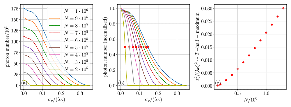
Figure 2. Photon number dependence on temperature and atom number.
(a) steady state photon number (mean field, see Appendix for comparison to higher orders) as a function of the standard deviation of the velocity distribution σv for different atom numbers. (b) Photon number normalized to σv = 0 (maximum). The red dots indicate the value at which the curves have dropped to half of their initial value. After normalizing, the curves do not longer align, hinting to a nonlinear relation between atom and photon number. (c) Dependence of the threshold value of the velocity spread on the number of atoms. Larger atom numbers allow for larger possible values of σv, while maintaining a lot of photons inside the cavity. The parameters are ν = 0.5, ∆ = 0, g = 0.00136 and κ = 1. We neglect γ since it is much smaller than ν, see Equation (6).
Adding a velocity filter
An interesting idea is to consider a cutoff in the velocity distribution for the atoms. Experimentally, this may be achieved by using a velocity filter for the atomic beam to get rid of the atoms with very high velocity, creating a smaller but colder ensemble. This could be more advantageous than trying to narrow the velocity distribution by cooling, as cooling the atoms proposes an experimental challenge. To simulate such a filter, we start with the same number of atoms as before, but exclude all atoms from the dynamics with velocities higher than the cutoff. We depict the results in Figure 3 for a cutoff at σv (≈ 68% slowest atoms) and at σv/2 (≈ 38% slowest atoms). To compare, we also depict the previous results without cutoff. In Figure 3(a) the steady state photon number is shown for the different cutoffs. By cutting off the high velocity part of the atomic distribution, we lose only fast atoms, but it always leads to a decrease in photon number. A velocity filter therefore only reduces the photon number. It might still be useful with respect to the linewidth, which is not calculated at this point.
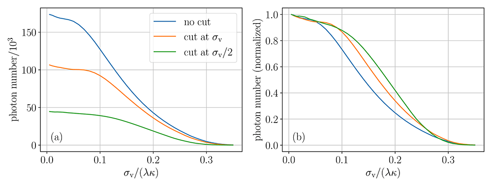
Figure 3. Photon number for different velocity cutoffs.
(a) Mean steady state photon number. (b) Normalized to maximum photon number. Cutting off the the high velocity part of the distribution always yields a smaller steady state photon number, but it remains at a high level for increasing σv. We only depict the results in mean field, as the results in mixed order almost perfectly align. The parameters are the same as in Figure 2.
However, the photon number seems to be more stable with increasing temperature, which can be seen in Figure 3(b), where we normalize the graphs to their highest photon number (at zero temperature). While the photon number significantly drops already for low temperature (e.g. σv ≈ 0.1) for the uncut case, it stays relatively stable for the other cases, where we exclude the fast atoms.
In summary, including a velocity filter will negatively affect the photon number, but allow it to stay at a relatively stable value for low temperatures. However, it remains to be seen what effect such a velocity filter has on the linewidth of the atoms. In general, one would expect a velocity filter to be beneficial for the linewidth reduction, as the excluded, fast atoms increase the linewidth by means of the Doppler effect.
Dynamics including an optical lattice potential
So far, we assumed that the atoms move freely without any potential. After some time at non-zero temperature, the atoms will be randomly distributed over the mode function. To compare that situation to the zero-temperature case with non-moving atoms, we always place the atoms equidistantly distributed over the mode function. Therefore, the differences in photon number stem from the movement of the atoms itself, not from the somewhat artificial location of atoms on the mode function. The coupling between atoms and cavity field can be controlled (at least for low temperature) by including an optical lattice potential, as the atoms are trapped at the potential minimums. Aligning these potential minimums with the anti-nodes of the mode function leads to enhanced coupling compared to the random sampling of the mode function in the case where atoms move freely. The potential V (x) has the form with spatial periodicity λlatt and energy barrier ∆E. By using the Hamiltonian formalism one ends up with two linear differential equations of first order for each cluster. These additional equations can simply be added to the equations in the mean field (6) for simulation purposes. To keep the computation time low, we now simulated only NCl = 100 clusters instead of 400 and only averaged over 10 trajectories instead of 50.
For the optimal case, we assume an optical potential with exactly half the wavelength of the mode function, that way the minima of the optical potential are situated at the maximum values of |f(xm)|. The results of such a simulation are depicted in Figure 4(a). To compare to the previous results, we include the graph that we already calculated, which is the result for an energy barrier of ∆E = 0. The energy is expressed in terms of the recoil energy , where k = 2π/λ, vrec is the associated recoil velocity and m is the mass of the atoms. To get exemplary values for these energy scales we use the 40Ca intercombination line between 1S0 and 3P1 with λ = 657 nm and Γ = 2π · 375 Hz, the cavity linewidth is κ = 2π • 120 kHz. To compare the two energy scales of the energy barrier and the velocity of the atoms, we color the data points according to the fraction of trapped atoms at each particular energy barrier and velocity. For high energy barriers and low velocities we have a lot of trapped atoms, these data points are colored blue, whereas for low energy barriers and high velocities almost no atoms are trapped, these points are colored yellow. As we can see from Figure 4, the results change significantly by including a barrier. Let us first look at the case of low velocities/low temperatures: When the barrier is sufficiently high, then almost all the atoms are trapped at the antinodes of the mode function, leading to high coupling between atoms and cavities and eventually to higher photon number. For higher velocities/temperature, the number of photons stays significantly above the comparison graph for no energy barrier. On the one hand, this is because there are still atoms, that are trapped near the antinode of the mode function. On the other hand, there is a different effect at play, of which we can get a better insight when choosing the wavelength of the lattice slightly different from the wavelength of the mode function. Such a system may be of interest, as there usually is a mismatch between the effective optical lattice periodicity and the optical wavelength.
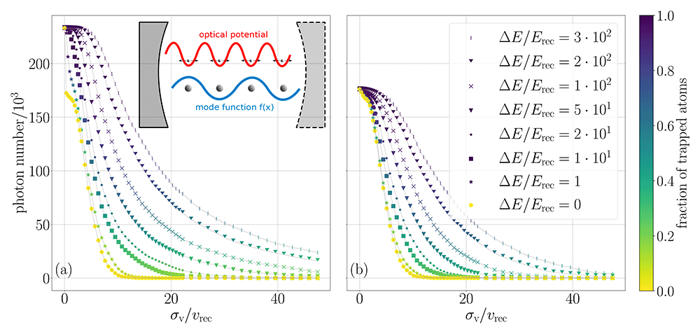
Figure 4.
Quasi-steady state photon number including an optical lattice potential with wavelength λlatt = 0.5 λ (a) and λlatt = 0.99 λ (b) with varying energy barriers. The color of the data points indicates the fraction of trapped atoms, where at blue most of the atoms are trapped, while at yellow most of the atoms can escape their trap. (a) λlatt = 0.5 λ: Due to the choice of λlatt, for low temperatures most of the atoms are trapped at the antinode of the mode-function, leading to a higher atom-cavity coupling and higher photon number. For higher temperatures, most of the atoms escape their trap, but the photon number stays significantly above the barrierless case. This is due to the energy barriers, which slow the atoms down, yielding lower Doppler effect and therefore higher photon number. (b) λlatt = 0.99 λ: For low temperatures the results coincide, regardless of the chosen energy barrier. This means, that the atom-cavity coupling is the same as in the barrierless case, where we distributed the atoms equidistantly over a mode function. For higher temperatures, most of the atoms escape their trap, but the photon number behaves similarly to the case with λlatt = 0.5 λ. Once again, the atoms get slowed by the barrier, eventually leading to significantly higher photon number compared to the barrierless case. The parameters are the same as in Figure 2.
The results can be seen in Figure 4(b), where we chose λlatt = 0.99λ. Note, how the results converge for very low temperature, regardless of the value of the energy barrier ∆E. This means, that the coupling is the same as in the barrierless case, where we distributed the atoms equidistantly over the mode function. So by choosing the wavelength of the optical lattice only slightly different to the wavelength of the mode function, we once again sample an average over the mode function, as long as the atoms sit on sufficiently many sites. Therefore the whole advantage of keeping atoms near the antinode of the mode function disappears and the coupling between the atoms and the cavity is the same compared to the coupling in the barrierless case. However, increasing the temperature, we still see a significant difference: Even though the average coupling is the same, the photon number is much higher. The atoms are decelerated, whenever they go over a potential barrier, yielding a reduced average velocity, which in turn decreases the Doppler effect and increases the photon number.
In summary, for low velocities/temperatures, the change in photon number depends mostly on the change of coupling of the atoms, which again depends on the location of the minima of the optical potential compared to the antinodes of the mode function. For higher velocities/temperatures, the other effect of having a lower average velocity due to the barriers comes also into play. The lower average velocity leads to a decreased Doppler effect and therefore a significant increase of photon number.
Conclusions
We studied incoherently pumped two-level-atoms inside a single mode cavity. In particular, we investigated the influence of temperature on the photon number. For high temperatures, where the atoms are fast, the photon number is suppressed because of the Doppler effect. However, we saw that increasing the atom number, to get sufficient collective atom-cavity-coupling, can compensate this suppression. Including a velocity filter leads to a lower amount of atoms participating in the dynamics and therefore, as the number of atoms is a significant parameter, to a lower photon number. We plan to calculate the spectrum to see if excluding the fast atoms has a decreasing effect on the linewidth.
With an optical lattice potential the coupling between the atoms and the cavity field can be controlled. For low temperatures (compared to the energy barrier), most atoms are trapped and the atom-cavity coupling (and in consequence the photon number) can be engineered. However, for high temperatures, even though most of the atoms are not trapped, the photon number significantly increases compared to the situation without a potential. In some cases, where virtually no photons are generated anymore for a certain σv without the potential, we still have a macroscopic photon occupation number, even if σv is 4 times as high, by including the optical potential. Therefore including an optical potential becomes very beneficial for higher temperatures.
Appendix. Equations in higher orders
As mentioned in the main text, for our parameter regime the physics is accurately described by mean field. To verify this, we derive the equations for higher orders in the cumulant expansion and compare the numerical results with the mean field. For second order, one derives equations for two-operator averages. These will depend on other averages of two-operator and three-operator products. In order to close the set of differential equations one needs to derive equations for the two-operator averages and approximate the three-operator averages according to 43
Using the phase invariance of the system5,44 one ends up with the set of equations in second order of the cumulant expansion:
The advantage of this second order is, that we can include atom-field and atom-atom correlations, however, we pay the price in form of a higher computation time, as the number of equations now scales quadratically with the cluster number instead of linearly as above. The terms involving two atom operators 〈σiσj〉 are responsible for the quadratic scaling, as both i and j are between 1 and N. In an attempt to take the advantage of the upsides of both first order and second order, we approximate two-operator products if they both are atom operators by splitting them, but keep the correlations between atom and field, we call this particular truncation "mixed order":
For the sake of better readability we refrain from carrying out all the expansions of three-operator expectation values like . In order to end up with a closed set of equations, one needs to approximate the three-operator expectation values by two-operator expectation values according to Equation (7). By neglecting the atom-atom correlations we get rid of the quadratic scaling, but we are still able to keep higher order correlations, namely the ones between atom and field. Grouping the atoms into clusters is more involved in the second order and mixed order as opposed to first order, one has to carefully take into account for example the correlations within a cluster17,45.
Determining the steady state photon number
In order to study the photon number values depending on different parameters we initialize the set of differential equations with a certain parameter set and let the system evolve until it reaches its quasi-steady-state. The velocities are drawn from a Gaussian distribution with width σv corresponding to a temperature. We average over the photon number from the timepoint, at which the quasi-steady-state has been reached, see Figure 5. Using more clusters leads to much smaller fluctuations, however, this also requires more computation time. Finding a compromise between high clusternumbers and reasonable computation time is discussed in the next section. Moreover, one can imagine that certain samples of the distribution exhibit special properties, in order to average them out we use 50 (unless indicated otherwise) different samples and also average over them.
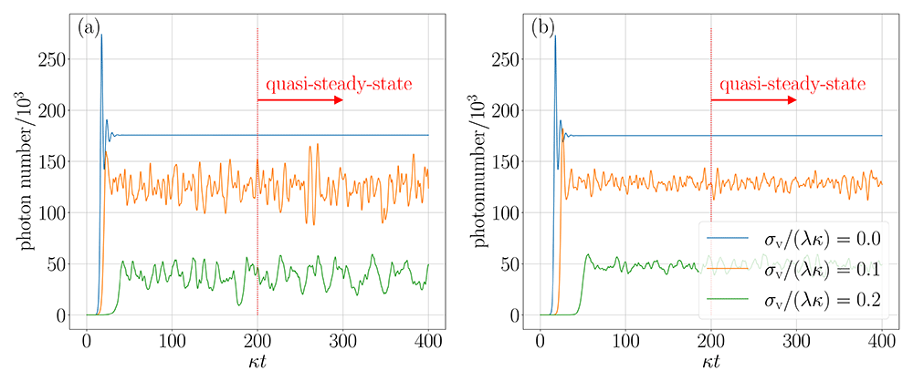
Figure 5. Determining the steady state photon number.
Mean photon number time evolution for different σv with (a) 200 atom clusters and (b) 1000 atom clusters. After a certain time, the system reaches its quasi steady state. The fluctuations become smaller if we divide the velocity distribution into a larger number of atom clusters. The other parameters are the same as in Figure 2 for N = 106.
Comparison expansion orders and number of clusters
Limited computation time forces us to make compromises, as both higher expansion orders and higher number of clusters describe the physical reality better, but also require more computation time.
In the following we compare the results for different expansion orders and number of cluster. In Figure 6(a) the solid line depicts the first order, the dotted line mixed order and the dashed line represents the data in second order. We see that all three lines almost perfectly align. Therefore, using higher expansion orders does not lead to significant differences and the first order approximation captures the essential physics in our parameter regime.
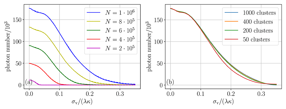
Figure 6. Expansion orders and number of clusters.
(a) The solid line represents mean field, the dotted line is mixed order and the dashed line depicts the result in second order, we use NCl = 25. The results for all orders agree very well. (b) The chosen number of clusters NCl makes a difference, especially for medium temperatures. However, increasing the number of clusters from NCl ≈ 400 has only a marginal effect on the results. The other parameters are the same as in Figure 2 for N = 106.
In Figure 6(b) we depict the results in first order for different clusternumbers ranging from NCl = 50 to NCl = 1000. Here we see, that varying the number of clusters NCl does have an influence on the results. We chose NCl = 400, as the difference between choosing NCl = 400 and as high as NCl = 1000 is only marginal, while the computation time significantly increases.
Faculty Opinions recommendedReferences
- 1.
Takamoto M, Hong FL, Higashi R, et al.:
An optical lattice clock.
Nature.
2005; 435(7040): 321–324. PubMed Abstract
| Publisher Full Text
- 2.
Bloom B, Nicholson TL, Williams JR, et al.:
An optical lattice clock with accuracy and stability at the 10-18 level.
Nature.
2014; 506(7486): 71–75. PubMed Abstract
| Publisher Full Text
- 3.
Ludlow AD, Boyd MM, Ye J, et al.:
Optical atomic clocks.
Rev Mod Phys.
2015; 87(2): 637. Publisher Full Text
- 4.
Haake F, Kolobov MI, Fabre C, et al.:
Superradiant laser.
Phys Rev Lett.
1993; 71(7): 995–998. PubMed Abstract
| Publisher Full Text
- 5.
Meiser D, Ye J, Carlson DR, et al.:
Prospects for a millihertz-linewidth laser.
Phys Rev Lett.
2009; 102(16): 163601. PubMed Abstract
| Publisher Full Text
- 6.
Chen J:
Active optical clock.
Chin Sci Bull.
2009; 54(3): 348–352. Publisher Full Text
- 7.
Meiser D, Holland M:
Steady-state superradiance with alkaline-earth-metal atoms.
Phys Rev A.
2010; 81(3): 033847. Publisher Full Text
- 8.
Meiser D, Holland M:
Intensity fluctuations in steady-state superradiance.
Phys Rev A.
2010; 81(6): 063827. Publisher Full Text
- 9.
Bohnet JG, Chen Z, Weiner JM, et al.:
A steady-state superradiant laser with less than one intracavity photon.
Nature.
2012; 484(7392): 78–81. PubMed Abstract
| Publisher Full Text
- 10.
Vuletic V:
Atomic physics: An almost lightless laser.
Nature.
2012; 484(7392): 43–44. PubMed Abstract
| Publisher Full Text
- 11.
Maier T, Kraemer S, Ostermann L, et al.:
A superradiant clock laser on a magic wavelength optical lattice.
Opt Express.
2014; 22(11): 13269–13279. PubMed Abstract
| Publisher Full Text
- 12.
Zhang Y, Zhang YX, Mølmer K:
Monte-carlo simulations of superradiant lasing.
New J Phys.
2018; 20: 112001. Publisher Full Text
- 13.
Debnath K, Zhang Y, Mølmer K:
Lasing in the superradiant crossover regime.
Phys Rev A.
2018; 98(6): 063837. Publisher Full Text
- 14.
Hotter C, Plankensteiner D, Ostermann L, et al.:
Superradiant cooling, trapping, and lasing of dipole-interacting clock atoms.
Opt Express.
2019; 27(22): 31193–31206. PubMed Abstract
| Publisher Full Text
- 15.
Gogyan A, Kazakov G, Bober M, et al.:
Characterisation and feasibility study for superradiant lasing in 40ca atoms.
Opt Express.
2020; 28(5): 6881–6892. PubMed Abstract
| Publisher Full Text
- 16.
Zhang Y, Shan C, Mølmer K:
Ultranarrow superradiant lasing by dark atom-photon dressed states.
Phys Rev Lett.
2021; 126(12): 123602. PubMed Abstract
| Publisher Full Text
- 17.
Bychek A, Hotter C, Plankensteiner D, et al.:
Superradiant lasing in inhomogeneously broadened ensembles with spatially varying coupling [version 2; peer review: 2 approved].
Open Res Eur.
2021; 1(73): 73. PubMed Abstract
| Publisher Full Text
| Free Full Text
- 18.
Kazakov GA, Dubey S, Bychek A, et al.:
Ultimate stability of active optical frequency standards.
Phys Rev A.
2022; 106: 053114. Publisher Full Text
- 19.
Kristensen SL, Bohr E, Robinson-Tait J, et al.:
Subnatural linewidth superradiant lasing with cold 88atoms.
Phys Rev Lett.
2023; 130(22): 223402. PubMed Abstract
| Publisher Full Text
- 20.
Zhang J, Shi T, Miao J, et al.:
The development of active optical clock.
AAPPS Bull.
2023; 33(1): 10. Publisher Full Text
- 21.
Goldenberg HM, Kleppner D, Ramsey NF:
Atomic hydrogen maser.
Phys Rev Lett.
1960; 5(8): 361–362. Publisher Full Text
- 22.
Kazakov GA, Schumm T:
Active optical frequency standard using sequential coupling of atomic ensembles.
Phys Rev A.
2013; 87(1): 013821. Publisher Full Text
- 23.
Kazakov GA, Schumm T:
Active optical frequency standards using cold atoms: Perspectives and challenges. In: 2014 European Frequency and Time Forum (EFTF). 2014; 411–414. Publisher Full Text
- 24.
Tang M, Schäffer SA, Müller JH:
Prospects of a superradiant laser based on a thermal or guided beam of 88Sr.
Phys Rev A.
2022; 106(6): 063704. Publisher Full Text
- 25.
Salzburger T, Ritsch H:
Atom-photon pair laser.
Phys Rev A.
2007; 75(6): 061601. Publisher Full Text
- 26.
Holland M, Burnett K, Gardiner C, et al.:
Theory of an atom laser.
Phys Rev A.
1996; 54(3): R1757–R1760. PubMed Abstract
| Publisher Full Text
- 27.
Hotter C, Plankensteiner D, Kazakov G, et al.:
Continuous multi-step pumping of the optical clock transition in alkaline-earth atoms with minimal perturbation.
Opt Express.
2022; 30(4): 5553–5568. PubMed Abstract
| Publisher Full Text
- 28.
Bennetts S, Chen CC, Pasquiou B, et al.:
Steady-state magneto-optical trap with 100-fold improved phase-space density.
Phys Rev Lett.
2017; 119(22): 223202. PubMed Abstract
| Publisher Full Text
- 29.
Chen CC, Bennetts S, Escudero RG, et al.:
Continuous guided strontium beam with high phase-space density.
Phys Rev Appl.
2019; 12(4): 044014. Publisher Full Text
- 30.
Escudero RG, Chen CC, Bennetts S, et al.:
Steady-state magneto-optical trap of fermionic strontium on a narrow-line transition.
Phys Rev Res.
2021; 3(3): 033159. Publisher Full Text
- 31.
Chen CC, Escudero RG, Minář J, et al.:
Continuous bose-einstein condensation.
Nature.
2022; 606(7915): 683–687. PubMed Abstract
| Publisher Full Text
| Free Full Text
- 32.
Norcia MA, Winchester MN, Cline JRK, et al.:
Superradiance on the millihertz linewidth strontium clock transition.
Sci Adv.
2016; 2(10): e1601231. PubMed Abstract
| Publisher Full Text
| Free Full Text
- 33.
Norcia MA, Thompson JK:
Cold-strontium laser in the superradiant crossover regime.
Phys Rev X.
2016; 6(1): 011025. Publisher Full Text
- 34.
Norcia MA, Cline JRK, Muniz JA, et al.:
Frequency measurements of superradiance from the strontium clock transition.
Phys Rev X.
2018; 8(2): 021036. Publisher Full Text
- 35.
Laske T, Winter H, Hemmerich A:
Pulse delay time statistics in a superradiant laser with calcium atoms.
Phys Rev Lett.
2019; 123(10): 103601. PubMed Abstract
| Publisher Full Text
- 36.
Schäffer SA, Tang M, Henriksen MR, et al.:
Lasing on a narrow transition in a cold thermal strontium ensemble.
Phys Rev A.
2020; 101(1): 013819. Publisher Full Text
- 37.
Tang M, Schäffer SA, Jørgensen AA, et al.:
Cavity-immune spectral features in the pulsed superradiant crossover regime.
Phys Rev Research.
2021; 3(3): 033258. Publisher Full Text
- 38.
Hotter C, Ostermann L, Ritsch H:
Cavity sub- and superradiance for transversely driven atomic ensembles.
Phys Rev Res.
2023; 5(1): 013056. Publisher Full Text
- 39.
Bohr E, Kristensen SL, Hotter C, et al.:
Collectively enhanced ramsey readout by cavity sub- to superradiant transition.
arXiv preprint arXiv: 2306.12544.
2023. Publisher Full Text
- 40.
Liu H, Jäger SB, Yu X, et al.:
Rugged mhz-linewidth superradiant laser driven by a hot atomic beam.
Phys Rev Lett.
2020; 125(25): 253602. PubMed Abstract
| Publisher Full Text
- 41.
Jäger SB, Liu H, Shankar A, et al.:
Regular and bistable steady-state superradiant phases of an atomic beam traversing an optical cavity.
Phys Rev A.
2021; 103(1): 013720. Publisher Full Text
- 42.
Jäger SB, Liu H, Cooper J, et al.:
Superradiant emission of a thermal atomic beam into an optical cavity.
Phys Rev A.
2021; 104(3): 033711. Publisher Full Text
- 43.
Kubo R:
Generalized cumulant expansion method.
J Phys Soc Jpn.
1962; 17(7): 1100–1120. Publisher Full Text
- 44.
Plankensteiner D, Hotter C, Ritsch H:
Quantumcumulants.jl: A julia framework for generalized mean-field equations in open quantum systems. 2021. Reference Source
- 45.
Fasser M:
Simulating a superradiant laser based on a thermal atomic beam. Master’s thesis, University of Inns- bruck, Innsbruck, Austria, 3.
2022. Reference Source
- 46.
Fasser M:
Superradiant_laser_figures.
Figshare.
2023. http://www.doi.org/10.6084/m9.figshare.c.6781920.v1
- 47.
Fasser M:
Srl_paper.
Zenodo.
2023. http://www.doi.org/10.5281/zenodo.8232295