Introduction
The size of current transistors is in the range of tens of nanometers, and such ultra-scaled dimensions pose many fabrication challenges1,2. One challenge is finding the best way to connect the transistors, as in the best interconnect material and mode. The current industrial standard is to fabricate the interconnect using many conducting layers of metals and their alloys (e.g. Cu and Ru)3,4. However, metal interconnects offer their own challenges at such small scales such as being bound by the aspect ratio limit in bit rate capacity and cross talk between different electrical lines5.
To overcome some of these issues, there is growing interest in substituting metal with miniaturized active photonic components for short-range optical interconnects5–7. Materials such as III-V semiconductors are known for their superior light adsorption and emission qualities8,9. They are currently integrated on silicon (Si) substrates with pick-and-place10 or wafer bonding methods11. This allows manufacturers to avoid defects related to lattice mismatch but limits integration density and alignment precision12,13. Monolithic growth of III-V semiconductors on Si can achieve quick, high-precision, simultaneous integration on large wafer scales.
Template assisted selective epitaxy (TASE) allows high defect control when growing III-V nano- and microstructures monolithically on silicon14,15. Analysis of the evolution of the growth front in TASE-grown heterostructured III-V nanowires is fundamental to ensure homogeneous heterolayer thickness16 and composition, in the case of ternary III-V compounds17. Achieving high uniformity across the entire wafer surface is critical, as these factors affect the optical behavior of the device.
Heterostructured III-V micro- and nanostructures are usually analyzed using scanning transmission electron microscopy (STEM) to determine the evolution and stability of the growth front18,19, as well as the presence of crystalline defects20,21. STEM analysis has shown19 that stabilization of the growth front tends to occur early in the growth process. This stabilisation improves the growth rate and geometry uniformity in TASE grown III-V nanowire. As a result, contact design is simplified, compared to previous experimental results where the metallic deposition area had to be defined on a wire by wide basis16. However, sample preparation for STEM is long and destructive22, making scanning electron microscopy (SEM) preferable for yield and reproducibility studies.
For the samples presented in this work, we selected growth conditions that stabilize a single {1 1 1} facet as a growth front perpendicular to the wafer surface for nanowires containing heterolayers of InP and InGaAs grown directly from a silicon seed19,23. From this knowledge, it is already possible to classify the wires as perfect from an SEM top-down view of the wire if the seed facet and the end facet are parallel along the growth direction and as defective otherwise.
When growing densely integrated submicrometer-sized III-V crystals, the current approach of manually cataloguing different growth outcomes on even a 2 cm × 2 cm chip becomes a very time-consuming and tedious process. One way to decrease the time requirements of such a study is to use machine learning (ML) methods. ML is a powerful tool for handling large amounts of data and has found application in materials science for various tasks. Classification24,25 and segmentation20 of electron microscopy images can be used to deduce device properties, if the images contain sufficient information26. ML models for identifying different types of nanostructures, such as the difference between nanowires, nanoparticles, and nanoporous substrates, have been shown to have extremely high accuracy27. However, models that are tasked with segmentation often do not perform as well28.
Classifying images containing multiple objects with fine differences is complex because the variability between nanowire images is of the same magnitude and quality as the target imperfections. Additionally, SEM images contain a high degree of noise that impedes the performance of traditional classification methods29. Due to the large number of images, this process can benefit from automatization30, especially when the need to use a less resolved and time-consuming characterization method arises31.
Hence, to tackle some of the abovementioned problems, we describe a novel ML-based approach in this paper. For the purpose of this work, we introduce and characterize a new dataset for nanowire classification. Finally, we evaluate the performance of our method on the aforementioned dataset and discuss future research areas.
This article makes the following contributions to the current state of the art:
1) To the best of our knowledge, this work shows the first kernel-based splitting algorithm for III-V nanowire array SEM images.
2) Our work provides a new nanowire classification dataset containing annotated images of III-V nanowire arrays.
3) In this work we demonstrate the performance of a compact convolutional neural network (CNN) classifier on the aforementioned dataset.
Methods
To extract individual nanowires for classification from each SEM image, we developed a novel algorithm that finds the location of each nanowire and extracts it32. The following algorithms were written in Python 3.933, using OpenCV34,35 as the image manipulation package. The algorithm locates the nanowires and is based on two kernel operations applied to an image. These operations minimize the effects of noise and enhance wire edges. The kernel manipulations used are similar to, but distinct from, the typical definition used in machine learning. In this approach, the kernel operates in situ and transforms an image into a filter to locate feature edges. Once the edges are located, we split the image into granular blocks and condition each image through histogram equalization. This produces the final input to the ML model. The entire pipeline of operation is shown in Figure 1.
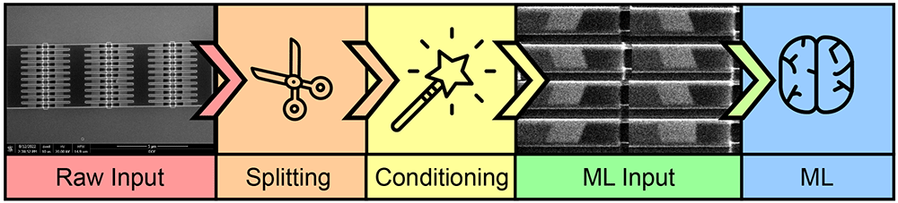
Figure 1. Process flow of classification method.
The raw input consists of scanning electron microscope (SEM) images divided into individual wires through a splitting algorithm. The wire images are conditioned and later used as the input for a convolution neural network (CNN) classifier in our machine learning (ML) method.
A. Kernel operations
As already discussed, our algorithm is based on two kernel operations. Both kernel operations are functions which act similarly. Each kernel searches for an extremum in a section of the image and then overwrites the whole section with the extremum value. Afterwards, the kernel moves along its row, ensuring an overlap between the previous and current window. At the end of a row, the kernel moves down the image and repeats the process without vertical overlap. This creates hard edges in the SEM image, removing any noise. Therefore, these operations find the rolling extremum in a row and propagate it forward. The two kernels find the minimum and maximum and are termed MinKernel and MaxKernel, respectively. The effect of these kernels on a noisy image is shown in Figure 2. There, it can be seen that the pixel values with the most extreme values are applied to the entire kernel and, due to the overlap, are extended to the end of the image.
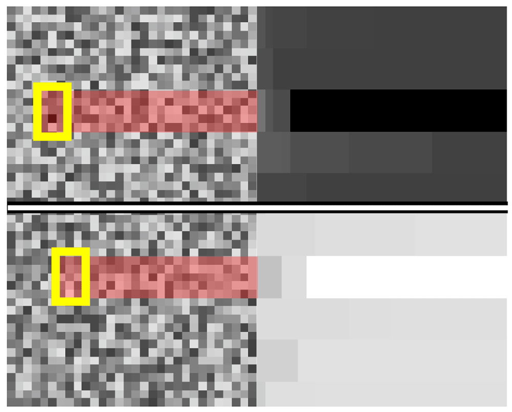
Figure 2. Mode of operation of kernel min and kernel max.
The application of the MinKernel is shown on the top row. The raw input from the left is transformed into the image on the right. The section with the darkest pixel value is highlighted. The application of the MaxKernel is shown on the bottom row. The raw input from the left is transformed into the image on the right. The section with the lightest pixel value is highlighted.
Algorithm
The algorithm splits up an image of an array, as in Figure 4, into its constituent nanowires by combining rotation, cut, split, and mirror operations. To simplify the nanowire isolation process, we have improved the cut operation to detect feature edges to cut around automatically. The operation is performed using information derived from MinKernel and MaxKernel. We devised a smart image paradigm that allows us to map a subsection of the visual domain onto its original coordinates and ultimately apply the cut on the original image for extraction. In this way, we can freely perform modifications, and once we determine the correct boundary, we can map back onto the original image and extract the nanowire picture. MinKernel and MaxKernel are used with gradient methods to identify where the cut point should be placed. The complete cut algorithm is shown in Algorithm 1.
Algorithm 1. Cut algorithm
Require: MinKernel
Require: MaxKernel
Require: Split(image, location or number of outputs)
Require: img - input image
images are treated as 2D arrays following right hand coordinate system
for each side do
minImg ← MinKernel(img)
maxImg ← MaxKernel(img)
for each col in maxImg do
maxV ← max(col)
end for
for each col in minImg do
minV ← min(col)
end for
maxGrad ←
minGrad ←
cutPoint1 ← arg maxx(maxGrad)
cutPoint2 ← arg maxx(minGrad)
img ← Split(img, min(cutPoint1, cutPoint2))[1]
rotate img by 90°
end for
return img
The full algorithm used to isolate a nanowire is shown in Algorithm 2. It involves cutting and rotating the image to isolate the main three-column array. Afterwards, one can split the array symmetrically into six parts. Then, each part is split again into eleven equally spaced rows. The base images are not perfectly aligned with the horizontal axis. Regardless, the algorithm works effectively for small degrees of tilt, up to 5°. For larger tilts, the methodology fails; however, as the environment is heavily controlled, the tilt in the images is significantly limited. Thus making our methodology suitable for use. Additionally, the rotation should not affect the classification accuracy since a wire’s features, which determine its class, are rotation-independent up to some allowable limit. The main features are how parallel the wire fronts are and the presence of a parasitic crystal growing on the surface of the wire.
Algorithm 2. Process algorithm
Require: MinKernel
Require: MaxKernel
Require: Cut(image)
Require: Split(image, location or number of outputs)
Require: img - input image of nanowire array
img ← Cut(img)
imgs ← Split(img, 6 columns)
wires ← empty list of nanowire images
for i in imgs do
i ← Cut(i)
tmpWires ← Split(i, 11 rows)
for j in tmpWires do
tmpWire ← Cut(j)
tmpWire ← Histogram equalization of tmpWire
Append tmpWire to wires
end for
end for
return wires
Machine learning model
The primary objective of this research paper is categorizing diverse visual representations depicting heterostructured nanowires. As previously mentioned, the pivotal impediment within this process pertains to the precise separation and extraction of nanowires from the base image. To demonstrate the efficacy of our pre-processing methodology, we have chosen to employ a compact image classification architecture implemented in the PyTorch framework (RRID:SCR 018536)36,37. The architectural configuration comprises a pair of convolutional layers succeeded by a trio of linear layers. The model structure is shown in Figure 3. The optimization process integrates the cross-entropy loss function with the Adam algorithm. Training was carried out for 100 iterations until loss saturation was achieved. The model uses a standard convolution approach, which has been used successfully to identify the class of images from popular datasets such as the CIFAR-1038.
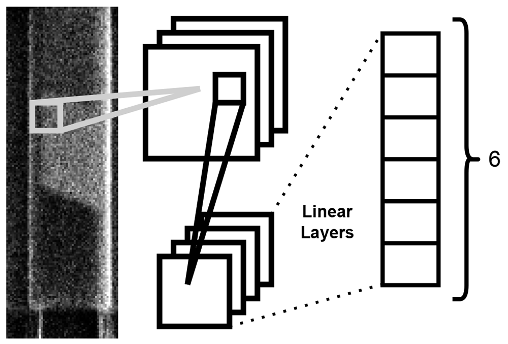
Figure 3. Diagram of the operation of the ML model used for nanowire classification.
Each nanowire image is fed through to two convolutional layers followed by three linear layers producing a final output of six probabilities.
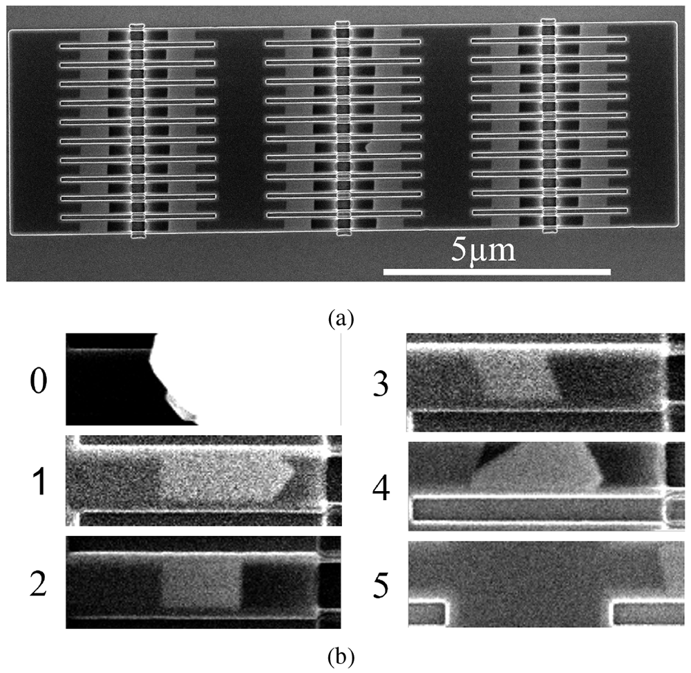
Figure 4. Scanning electron microscopy (SEM) images of two 11 × 6 nanowire arrays.
a) 210nm wide wires in a template parallel to a ⟨1 1 1⟩ in-plane direction. The wires appear as light grey segments. b) image portions representing each of the classes as cut by Algorithm 1.
Dataset
The dataset consists of 240 images containing arrays of 66 nanowires such as that presented in Figure 4a39, therefore, a total of 15840 nanowire nucleation sites are available in the dataset. 60% of the images contain arrays for the growth of wires in the “parallel” configuration and the remaining 40% consists of images of arrays in the “tilted” configuration. The wires were grown using TASE14,19,23. The images were captured with the electron beam of a FEI Helios NanoLab 450S in SEM mode. The arrays are made of different nanowire widths, with four sizes present: 70nm, 140nm, 210nm, 280nm, and in orientation with respect to the in-plane ⟨1 1 1⟩ directions. As the Si crystal determines the seed surface and the final facet orientation, changing the template orientation will produce a tilted seed and end facet (Figure 4b, class 3). SEM images are used for quality control in nanofabrication, as they allow for high magnification and survey speeds. Traditionally, once an SEM image is taken, the operator determines whether the nanowires contained in it are defective. We have surveyed the nanowire arrays and labelled them to produce the dataset used in this paper39.
The examples shown in Figure 4b provide an idea of what each class looks like. The wires were labelled using LabelMe40, with four classes used to capture the differences between the wires grown along a ⟨1 1 1⟩ direction and those grown tilted away from it (Table I). This produced the first four classes: ”Wire Parallel Perfect”, ”Wire Parallel Defect”, ”Wire Tilted Perfect”, and ”Wire Tilted Defect”. They represent 49.7%, 2.4%, 21.6%, and 1.6% of the dataset, respectively. Therefore, an imbalance exists between the number of defective and perfect wires, with the latter greatly outnumbering the former and an overall prevalence of the ”Wire Parallel Perfect” class in the dataset.
Table I. Class encodings.
| | Wire Parallel | Wire Tilted | |
|---|
| Class | Parasitic | Defect | Perfect | Defect | Perfect | Null |
| Encoding | 0 | 1 | 2 | 3 | 4 | 5 |
A fifth class is necessary because of the presence of parasitic growth on the surface of some arrays. Parasitic growth occurs on the rare occasion when III-V material nucleates on the walls of the template SiO2. As there is no template to contain the growth of this parasitic crystal, it expands faster, covering a large number of templates.
A ”Null” class is introduced to take into account the possibility that the pre-processing algorithm could have sliced the image incorrectly. This can be due to a number of factors, such as a tilt of a few degrees of the structure in the image or the influence of a large parasitic growth crystal in the cutting of the array contours. The percentage of ”Null” class images in the dataset was calculated at 12.6%.
Experiment set-up
We divide the data set into training and validation sets with a 70/30 split. We trained the model for 100 epochs. The training loss is shown to saturate around 100 epochs in Figure 5, indicating the successful training of the model. Two metrics, precision and recall, are used to evaluate the performance of a classifier when encountering new data that it was not presented with, during the training stage. Precision and recall refer to the ability of the model to correctly identify an item in the test set as belonging to a class. Precision is the ratio of true positives to the sum of true and false positives. Recall, on the other hand, is defined as the ratio of true positives to the sum of true positives and false negatives. Precision and recall can be combined into the F1 score, a metric that gives an overall assessment of the quality of the model. The F1 score of the best model was recorded on the test set at 0.91 ± 0.04 (97% confidence).
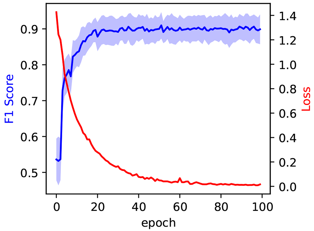
Figure 5. In blue, the evolution of the F1 score during model training, measured on the test set at each epoch.
The blue shaded area corresponds to the 97% confidence interval. The evolution of the training loss is measured on the training set at each epoch and reported in red.
In some circumstances, such as when an imbalanced dataset is employed, a single number metric such as the F1 score can, however, give a misleading or incomplete ”idea” of the model’s performance. In such a situation, per-class metrics provide greater insight into a model’s performance. The confusion matrix in Figure 6 summarizes the per-class performance of the model. The distribution of the predictions for each class is shown on each row. The data is presented as percentages: as such, the diagonal (top left to bottom right) also indicates the percentage recall of each class.
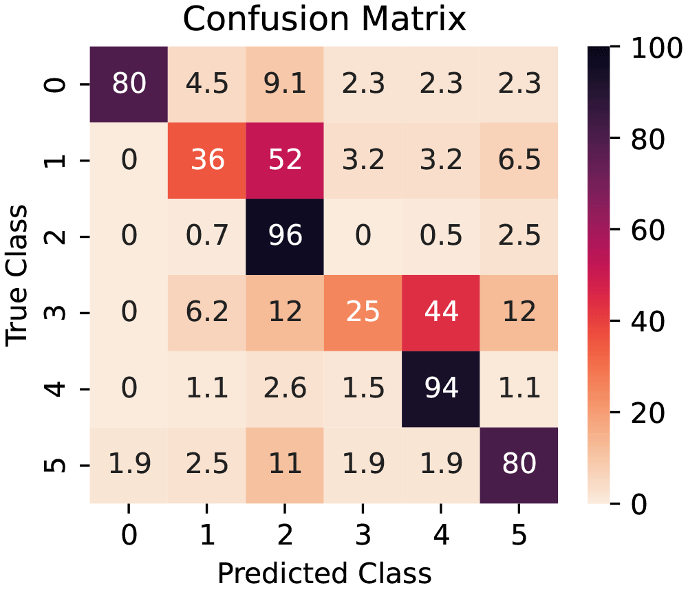
Figure 6. Confusion matrix for the model (from test set).
The values are row-normalized and presented as percentages.
Results
The model shows outstanding performance in nanowire classification: achieving a total F1 score of 0.91 ± 0.04. This surpasses similar methods for nanowire classification by roughly 0.130 while using a more compact model with lower computational costs. The model shows excellent overall performance, exemplified by the high F1 score of 0.91 ± 0.04 obtained from training on an original dataset of only 240 images. The F1 Score saturates early in the training process, after around 30 epochs, as is evident by the blue curve in Figure 5.
The model’s performance is different depending on the class it is trying to predict. The Recalls for each class are represented in the diagonal elements of the confusion matrix in Figure 6 and illustrate how the model performs when distinguishing between different classes. It can easily distinguish between non-defective parallel and tilted wires and reliably identify wrongly cut images containing partial III-V nanowires (non-defective class) or parasitic crystals. However, the model struggles to correctly classify defective wires in the test data set, with percentages of 36% and 5% of correctly identified parallel and tilted wires (classes 1 and 3). Conversely, defective wires are more likely to be classified as non-defective (52% and 44%). This is due to a combination of factors: there is a scarcity of defective wires in the data set, totaling less than 5% of the data, and growth failures can occur in more than one configuration, often with a small deviation from the desired shape creating the defect. Therefore, the preprocessing algorithm is not a contributing factor in this metric.
Conclusions
In this work, we have shown a novel algorithm to separate individual nanowires from nanowire arrays to create a general model to classify nanowires as defective and non-defective and differentiate between different growth configurations. We achieved an F1 score of 0.91 in the test set, and the recall and confusion matrix have shown a high competence in the distinction between parallel and tilted wires and parasitic growth.
Expanding the initial data set with more SEM images will likely help overcome the difficulties in classifying defective wires. We expect this expansion to not only aid in recognition of defective wires but also to be able to correctly classify tase wires grown with other crystalline orientations, given the current model’s ability to distinguish between parallel and tilted wires. Furthermore, in an industrial application where the tilt of the sample and the contrast and brightness are more homogeneous than the ones in the present dataset, the prevalence of the Null class is expected to be reduced. A more complex machine learning model could achieve better performance; however, our preprocessing approach has proven capable of creating an input dataset well suited for a lightweight model.
Our manual segmentation approach is particularly powerful, as it relies on precise image gathering, easily achievable with SEM instrumentation, and can be further enhanced by a data acquisition algorithm. The preprocessing algorithm has proven to be a robust way to extract single nanowire images, reducing the complexity of the machine learning model’s task. This produced a small, quick, and efficient model that has achieved a high degree of accuracy.
Ethics and consent
Ethical approval and consent were not required.
Acknowledgment
E. B. thanks the Cleanroom Operations Team of the Binning and Rohrer Nanotechnology Center for their help and support and Dr. Heinz Schmid for his support with MOCVD growth.
Faculty Opinions recommendedReferences
- 1.
Lee MW, Lin YC, Lai KH, et al.:
Study of AlGaN/GaN high-electron-mobility transistors on Si substrate with thick copper-metallized interconnects for Ka-band applications.
physica status solidi (a).
2023; 220(8): 2200536. Publisher Full Text
- 2.
Ciofi I, Contino A, Roussel PJ, et al.:
Impact of wire geometry on interconnect RC and circuit delay.
IEEE Trans Electron Devices.
2016; 63(6): 2488–2496. Publisher Full Text
- 3.
Wen LG, Adelmann C, Pedreira OV, et al.:
Ruthenium metallization for advanced interconnects.
2016 IEEE International Interconnect Technology Conference / Advanced Metallization Conference (IITC/AMC).
2016; 34–36. Publisher Full Text
- 4.
Mukesh S, Lanzillo NA:
A multiscale simulation study of the structural integrity of damascene interconnects in advanced technology nodes.
IEEE Trans Electron Devices.
2023; 70(4): 1977–1982. Publisher Full Text
- 5.
Miller DAB:
Rationale and challenges for optical interconnects to electronic chips.
Proceedings of the IEEE.
2000; 88(6): 728–749. Publisher Full Text
- 6.
Smit M, Williams K, van der Tol J:
Past, present, and future of InP-based photonic integration.
APL Photonics.
2019; 4: 050901. Publisher Full Text
- 7.
Miller DAB:
Attojoule optoelectronics for low-energy information processing and communications.
J Lightwave Technol.
2017; 35(3): 346–396. Publisher Full Text
- 8.
Wallentin J, Anttu N, Asoli D, et al.:
InP nanowire array solar cells achieving 13.8% efficiency by exceeding the ray optics limit.
Science.
2013; 339(6123): 1057–1060. PubMed Abstract
| Publisher Full Text
- 9.
Zhang G, Takiguchi M, Tateno K, et al.:
Telecom-band lasing in single InP/InAs heterostructure nanowires at room temperature.
Sci Adv.
2019; 5(2): eaat8896. PubMed Abstract
| Publisher Full Text
| Free Full Text
- 10.
McPhillimy J, Jevtics D, Guilhabert BJE, et al.:
Automated nanoscale absolute accuracy alignment system for transfer printing.
ACS Appl Nano Mater.
2020; 3(10): 10326–10332. PubMed Abstract
| Publisher Full Text
| Free Full Text
- 11.
Caimi D, Tiwari P, Sousa M, et al.:
Heterogeneous integration of III-V materials by direct wafer bonding for high-performance electronics and optoelectronics.
IEEE Trans Electron Devices.
2021; 68(7): 3149–3156. Publisher Full Text
- 12.
Tang M, Park JS, Wang Z, et al.:
Integration of III-V lasers on Si for Si photonics.
Prog Quantum Electron.
2019; 66: 1–18. Publisher Full Text
- 13.
Wang Z, Abbasi A, Dave U, et al.:
Novel light source integration approaches for silicon photonics.
Laser Photon Rev.
2017; 11(4): 1700063. Publisher Full Text
- 14.
Borg M, Schmid H, Moselund KE, et al.:
Mechanisms of template-assisted selective epitaxy of InAs nanowires on Si.
J Appl Phys.
2015; 117(14): 144303. Publisher Full Text
- 15.
Tiwari P, Triviño NV, Schmid H, et al.:
Review: III-V infrared emitters on Si: fabrication concepts, device architectures and down-scaling with a focus on template-assisted selective epitaxy.
Semicond Sci Technol.
2023; 38(5): 053001. Publisher Full Text
- 16.
Wen P, Tiwari P, Mauthe S, et al.:
Waveguide coupled III-V photodiodes monolithically integrated on Si.
Nat Commun.
2022; 13(1): 909. PubMed Abstract
| Publisher Full Text
| Free Full Text
- 17.
Borg M, Gignac L, Bruley J, et al.:
Facet-selective group-III incorporation in InGaAs template assisted selective epitaxy.
Nanotechnology.
2019; 30(8): 084004. PubMed Abstract
| Publisher Full Text
- 18.
Šuran Brunelli ST, Goswami A, Markman B, et al.:
Horizontal heterojunction integration via template-Assisted selective epitaxy.
Cryst Growth Des.
2019; 19(12): 7030–7035. Publisher Full Text
- 19.
Brugnolotto E, Scherrer M, Schmid H, et al.:
Growth of type I superlattice III-V heterostructure in horizontal nanowires enclosed in a silicon oxide template.
J Cryst Growth.
2023; 603: 127015. Publisher Full Text
- 20.
Dennler N, Foncubierta-Rodriguez A, Neupert T, et al.:
Learning-based defect recognition for quasi-periodic HRSTEM images.
Micron.
2021; 146: 103069. PubMed Abstract
| Publisher Full Text
- 21.
Arroyo Rojas Dasilva Y, Kozak R, Erni R, et al.:
Structural defects in cubic semiconductors characterized by aberration-corrected scanning transmission electron microscopy.
Ultramicroscopy.
2017; 176: 11–22. PubMed Abstract
| Publisher Full Text
- 22.
Cuti G, Jabbar T:
Automated S/TEM sample preparation for semiconductor process support.
Microscopy Today.
2018; 15(1): 26–29. Publisher Full Text
- 23.
Brugnolotto E, Schmid H, Georgiev V, et al.:
In-Plane III–V nanowires on Si(1 1 0) with quantum wells by selective epitaxy in templates. Cryst Growth Des.2023; 2311: 8034–8042. Publisher Full Text
- 24.
Modarres MH, Aversa R, Cozzini S, et al.:
Neural network for nanoscience scanning electron microscope image recognition.
Sci Rep.
2017; 7(1): 13282. PubMed Abstract
| Publisher Full Text
| Free Full Text
- 25.
Durmaz AR, Müller M, Lei B, et al.:
A deep learning approach for complex microstructure inference.
Nat Commun.
2021; 12(1): 6272. PubMed Abstract
| Publisher Full Text
| Free Full Text
- 26.
Zhang L, Shao S:
Image-based machine learning for materials science.
J Appl Phys.
2022; 132(10): 100701. Publisher Full Text
- 27.
Kavuran G:
SEM-Net: Deep features selections with Binary Particle Swarm Optimization Method for classification of scanning electron microscope images.
Mater Today Commun.
2021; 27: 102198. Publisher Full Text
- 28.
Lin B, Emami N, Santos DA, et al.:
A deep learned nanowire segmentation model using synthetic data augmentation.
npj Computational Materials.
2022; 8: 88. Publisher Full Text
- 29.
Yim J, Sohn KA:
Enhancing the performance of Convolutional Neural Networks on quality degraded datasets.
2017 International Conference on Digital Image Computing: Techniques and Applications (DICTA).
2017; 1–8. Publisher Full Text
- 30.
Lee B, Yoon S, Lee JW, et al.:
Statistical characterization of the morphologies of nanoparticles through machine learning based electron microscopy image analysis.
ACS Nano.
2020; 14(12): 17125–17133. PubMed Abstract
| Publisher Full Text
- 31.
Xu Y, Xu D, Yu N, et al.:
Machine learning enhanced optical microscopy for the rapid morphology characterization of silver nanoparticles.
ACS Appl Mater Interfaces.
2023; 15(14): 18244–18251. PubMed Abstract
| Publisher Full Text
- 32.
Brugnolotto E, Alexandrov P:
Image Classifier of Nanowire Arrays. 2023. http://www.doi.org/10.5281/zenodo.10255657
- 33.
Python programming language. (RRID:SCR 008394).
- 34.
OpenCV. (RRID:SCR 015526).
- 35.
Bradski G:
The OpenCV Library. In: Dr. Dobb’s Journal of Software Tools.
2000.
- 36.
PyTorch. (RRID:SCR 018536).
- 37.
Paszke A, et al.:
PyTorch: An Imperative Style, High-Performance Deep Learning Library. In: Advances in Neural Information Processing Systems. Curran Associates, Inc., 2019; 32. : 8024–8035.
- 38.
Krizhevsky A, Sutskever I, Hinton GE:
ImageNet Classification with Deep Convolutional Neural Networks. In: Advances in Neural Information Processing Systems. Ed. by F. Pereira et al., Curran Associates, Inc., 2012; 25. . Reference Source
- 39.
Brugnolotto E:
SEM Images of Arrays of III-V Nanowires with Labelled Data. 2023. http://www.doi.org/10.5281/zenodo.10204018
- 40.
Wada K: https://github.com/ wkentaro/labelme, 2016.