Introduction
An efficient membrane distillation (MD) process requires customized membranes with well-defined properties. The desired membranes should be porous and hydrophobic. MD is a thermally driven separation process where the membrane separates the feed solution (in our case salt water) into a highly concentrated salt solution (brine) and a cold distillate (permeate). The driving force of this separation process is therefore a temperature gradient that allows only water vapor to pass from the hot feed side with higher vapor pressure to the cold distillate side with lower vapor pressure. A hydrophobic porous material will therefore block the passage of liquid water by surface tension force while allowing the passage of water vapor (Hsu et al., 2002). Membrane porosity, along with pore size, are the other important factors influencing the process as they control the water flux. High porosity is often associated with large pore sizes, resulting in higher flux. However, large pore sizes favor pore wetting and thus salt permeation through the membrane. Membrane fabrication involves a favorable compromise between the membrane properties mentioned above. Phase inversion is commonly used to fabricate hydrophobic MD membranes.
Phase inversion processes are the most preferred for the preparation of polymeric membranes due to their ease of processing, flexible production scale and low cost [Barbe et al., 2020; Metze et al., 2017]. They can be classified into four main types, namely non-solvent induced phase separation (NIPS), thermally induced phase separation (TIPS), vapor induced phase separation (VIPS) and evaporation induced phase separation (EIPS). The NIPS technique, also known as wet phase inversion or immersion precipitation (IP), involves direct immersion of the cast polymer film in a non-solvent bath, also called a coagulation bath (Bohr et al., 2023). It is therefore considered to be a simple and convenient method for preparing polymer membranes. The immersion of the cast polymer film in the coagulation bath leads to rapid mass transfer and solvent/non-solvent exchange processes in the liquid phases, inducing membrane formation. This mechanism leads to anisotropic porous membranes, featuring a selective dense skin, and finger-like macrovoids throughout the cross-section of the support layer.
As mentioned above, membrane porosity is an important factor in MD performance. The dense skin formed in asymmetric membranes during NIPS acts as a barrier to the MD flux. Therefore, the skin and cross-sectional porosity must be increased. To this end, many studies have investigated the influence of additives on pore formation and pore interconnectivity. Several works have reported the preparation of polymeric membranes incorporating different additives, especially hydrophilic polymers such as polyvinylpyrrolidone (PVP) or polyethylene glycol (PEG) (Guillen et al., 2011). The results show that these additives lead to an improvement in membrane porosity and permeability, resulting in better MD performance. Tomaszewska et al. described the use of LiCl as a pore former to develop PVDF membranes for MD applications (Tomaszewska, 1996). The reported cross sections of pure PVDF membranes consisted of a dense top layer with underlying macrovoids and a sponge-like bottom layer. LiCl enlarged the macrovoids while the sponge-like sublayer disappeared. More recently, additives like carbon nanotubes (Kumar et al., 2019), silica nanoparticles (Aquino et al., 2018; Julian et al., 2019), and amphiphilic copolymers (Zhao et al., 2013) have been investigated. These additives have improved properties such as higher fouling resistance (Yi et al., 2012). The use of additives is now a common practice in the development of polymeric membranes to fine-tune their properties to better suit them for the applications for which they are designed.
In this context, AWC-embedded self-supporting flat sheet PVDF membranes have been developed. AWC are simple amphiphilic molecules, namely hexylureido-ethyl-imidazole (HC6), which are generating via self-assembly synthetic mimics of biological water channel proteins, aquaporins, allowing them to replicate their characteristic properties. These include the ability to combine high water permeability with high water/solute selectivity along with higher processability and stability compared to aquaporine channels (Di Vincenzo et al., 2021). The presence of AWC within the polymer matrix creates selective pathways through which water can flow freely, thereby accelerating permeate flux. In our previous publication, AWC-embedded PVDF membranes prepared by NIPS showed improved porosity and flux during the MD process compared to pure PVDF membranes (Nursiah et al., 2023).
The VIPS technique is an approach to membrane preparation that is well suited for MD applications. In contrast to NIPS, the non-solvent used in VIPS is in the vapor phase (usually water vapor). Phase separation is induced by exposing the cast polymer solution film to a non-solvent containing atmosphere. The polymer film is then immersed in a coagulation bath to complete the phase inversion and to wash out the remaining solvent. The main difference between NIPS and VIPS lies in the final membrane morphology, which is influenced by the mass transfer mechanism that occurs during the phase separation process. NIPS generally results in anisotropic porous membranes with a dense skin and finger-like macrovoids, whereas VIPS results in an isotropic sponge-like morphology with a more open porous surface. In NIPS, mass transfer occurs across a liquid-liquid phase boundary, whereas in VIPS, mass transfer occurs across a gas-liquid phase. It can be concluded that the difference in mass transfer during the two phase inversion processes is responsible for the change in membrane morphology. During NIPS, different experimental conditions such as polymer concentration, non-solvent coagulation bath temperature and non-solvent type were investigated to determine their influence on the mass transfer rate and consequently the morphology. VIPS adds relative humidity (RH) and exposure time to the list of process parameters. For example, Alexowsky recently demonstrated in his work that a bi-continuous (lacy) structured PVDF membrane can be achieved by controlling the RH and exposure time of the vapor phase (Alexowsky et al., 2019). Solvent selection plays an important role in membrane preparation during VIPS. Three key parameters should be considered when evaluating solvent selection: good solvency, appropriate viscosity, and low volatility (Tan & Rodrigue, 2019). For example, the highly porous structure observed in VIPS membranes can be demonstrated by the influence of solvent volatility as shown in the work of Su et al. (Su et al., 2009). However, the control of morphology during VIPS is also highly dependent on a number of other factors. For example, the polymer dissolution temperature Td has been described as critical to the final membrane morphology and mechanical stability. The morphology of the bicontinuous (lacy) structured membrane described in Alexowsky's research (Alexowsky et al., 2019) is the result of a careful choice of Td. This phenomenon is best explained by the phase separation mechanism, which clearly illustrates the critical role of Td in the final membrane morphology. The phase separation of the polymer solution occurs via two known mechanisms, namely the nucleation and growth mechanism (Lifshitz & Slyozov, 1961) and the spinodal decomposition mechanism (Cahn, 2004). The mechanism favored by phase separation depends on the position of its composition on the ternary thermodynamic phase diagram (Mulder, 1991), which is represented by three distinct regions: homogeneous, metastable, and unstable. A bi-continuous (lacy) structure is said to be obtained when the phase separation composition is in the unstable region. Spinodal decomposition is the preferred mechanism in this case (Cahn, 2004; Chung & Teoh, 1997). Further to this established description of the morphology of the bi-continuous (lacy) structure, Li et al. defined a critical dissolution temperature Tcd in their work (Li et al., 2010). They suggested the occurrence of a pronounced change in membrane morphology under VIPS conditions, depending on whether Td is above or below the defined Tcd. This morphological change is characterized by the crystallization of PVDF in its different crystalline phases, in particular the alpha and beta forms. It was found that the bi-continuous (lacy) structure, which exhibits high mechanical stability and is characterized by an excess of the alpha crystalline phase of PVDF, is favored when Td is below Tcd (Li et al., 2010). Li et al. also illustrate in their work the dependence of the minimum and critical dissolution temperatures on PVDF concentration (Li et al., 2010). Based on their results, the Td in the present work is higher than the Tcd. The phase separation process consisted of an initial VIPS stage of limited duration followed by a NIPS stage in an attempt to combine a porous bi-continuous (lacy) surface morphology with a highly porous finger-like sublayer while maintaining mechanical stability.
Combining the effect of increased water permeability of the AWC with the well-defined structure expected from the VIPS process is the main scope of the present work. In our previous work (Nursiah et al., 2023), the optimization of the AWC-embedded PVDF membrane by the NIPS process was achieved by varying the polymer concentration and the AWC concentration. The present study investigates the combined effect of the latter, as well as RH and exposure time, on the morphology and dynamic performance (PWP and MD flux) as well as the LEP of AWC-embedded PVDF membranes prepared by the VIPS method. To the best of our knowledge, only a few studies have applied DoE and RSM as a method for membrane optimization designed for MD. The work of Khayet et al. can be cited as one such example, where they report the use of RSM for the optimization of the MD process (Khayet et al., 2010). In fact, the one-factor-at-a-time (OFAT) method is the most commonly used experimental design method. In a classical experimental design, where multiple factors could influence the outcome, the OFAT method involves testing one factor at a time while the other parameters are fixed. For example, for the NIPS process, the two factors were polymer concentration and AWC concentration. The optimization of the AWC-embedded PVDF membranes was achieved by varying the concentration of one of the two factors while keeping the other fixed. On the other hand, in the VIPS process, it should be emphasized that the influence of four parameters on the morphology and MD performance of the prepared membranes should be investigated in order to identify the optimized AWC-embedded PVDF membrane. The conventional OFAT method could be a hurdle considering the high number of experimental runs required, not to mention the risk of ignoring possible interaction effects between the studied parameters. Therefore, a combination of DoE and RSM is proposed to analyze the interactions of the different factors simultaneously. Herein, based on this statistical approach, we report the preparation of AWC-embedded self-supported flat sheet PVDF membranes via the VIPS method, supported by a NIPS step, for Direct Contact Membrane Distillation (DCMD).
Methods
Materials
PVDF pellets (CAS No.: 24937-79-9; MW = 530 000 g/mol) and N,N-Dimethylacetamide (CAS No.: 127-19-5) were provided by Sigma-Aldrich Germany. Laboratory produced distilled water (18 MΩ.cm-1) was used as coagulation bath for membrane preparation and in the DCMD experiments. The HC6 AWC were synthesized according to a procedure described elsewhere (Le Duc et al., 2011). All experimental designs, their analyses and modelling were performed using Minitab v. 20.3.
Membrane preparation
VIPS-NIPS assisted membrane preparation was performed according to the following protocol. Dope solutions, with compositions summarized in Table 3, were prepared by dissolving the PVDF pellets in N,N-dimethylacetamide (DMAc) for 6 h at a dissolution temperature Td of 55°C, followed by a degassing period of 18 h at room temperature (22°C). The stainless-steel support used for solution casting was previously fixed in a vapor box maintained at room temperature with a circulating thermostat. Figure 1 shows a schematic of the experimental VIPS setup. The humid atmosphere in the chamber was controlled by a compressed air piping system consisting of two wet lines and one dry line. The wet lines each consisted of a 1 L double-jacketed glass frit impinger. Thus, the desired relative humidity (RH) in the vapor box was set by adjusting the air flow rates in the wet and dry lines. The temperature and air flow rate in the box were held constant at 22°C and 7.7 L/min, respectively, and the humidity and exposure time were varied according to the values specified by the DoE. The flow rate of the conditioned air stream, its relative humidity, and the pressure and temperature of the air stream were constantly monitored. The degassed dope solution was cast onto the support using a casting knife (Micrometer Adjust Applicator 400 mm) with a gap size of 250 µm. After casting, the vapor box was closed and the nascent membrane was exposed to humid air for the desired time. The support was then removed from the vapor box into a dry atmosphere (relative humidity <18%). The steel plate was immersed in a coagulation bath (distilled water at room temperature) for 24 h. The resulting membranes were dried in a stack. Each membrane was laid flat on a stainless-steel plate and held in place by four rectangular blocks of PTFE placed on each of the four edges. The plates with wet membrane sheets and blocks were then stacked. The PTFE blocks have horizontal holes so that a constant flow of dry air was blown horizontally through the stack by a fan to ensure a gentle and uniform drying process.
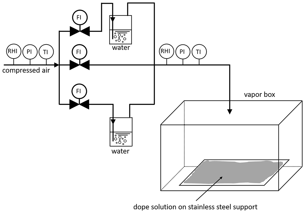
Figure 1. Schematic representation of VIPS setup used in this work.
Membrane characterization
Morphological analysis by Scanning Electron Microscopy (SEM). The top surface and cross-section of the membranes were examined by means of scanning electron microscopy (SEM). The images were taken with a MEB Hitachi S4800, with a resolution of 1 nm at 15 kV and capable of an acceleration voltage range of 0.1 kV to 30 kV.
Pure Water Permeability (PWP) and Liquid Entry Pressure (LEP). The PWP permeability measurements were carried out according to the following protocol, which is also described in detail in our previous work (Nursiah et al., 2023).
The LEP was determined together with the pure water permeability to characterize the wetting resistance of the membranes. For this purpose, a water-filled dead-end filtration setup was used. The membrane was placed inside the cell and the pressure applied on the feed side was increased stepwise in 0.1 bar increments after two minutes of stabilization time after each step. After reaching the LEP, the membrane was compressed at 4.0 bar for 45 min. After compression, the pressure was decreased in 0.5 bar increments and the water flux was recorded and plotted as a function of transmembrane pressure. The PWP of the membrane was determined by considering the gradient of the slope of the obtained linear relationship.
Direct Contact Membrane Distillation (DCMD). The DCMD performance was investigated according to the following protocol, as described in our previous work (Nursiah et al., 2023).
A pilot-scale MD setup was used for the DCMD experiments. The self-supporting flat sheet membranes were tightly clamped between two Teflon plates, leaving an effective operating area of 28.6 cm2. An aqueous sodium chloride solution (35 g/L) constituted the feed side, and the permeate was directly recovered in the circulating cooling system (18 MΩ.cm water). The feed inlet temperature Tf was fixed at 70°C (± 2°C) and the distillate inlet temperature Tp was maintained at 10°C (± 1°C). Two independent peristaltic pumps were used to circulate the feed and permeate sides. The pump for the former helped maintain a flow rate of 55 L/h. The main operating conditions used in the DCMD experiments are listed in Table 1.
Table 1. Operating conditions used in DCMD experiments.
| Parameter | Range |
|---|
Membrane module
Support
Feed temperature [°C]
Feed flow rate [L/h]
Permeate temperature [°C] | Flat
No
70 ± 2
55
10 ± 1 |
Throughout the DCMD process, the distilled permeate was diluted in the cold circulating water. The diluted solution was collected and weighed after an average period of 3 h 30 min. The salt concentration Cp collected in the distilled permeate was monitored by conductivity σ (S.m-1) (Conductometer VWR ® Phenomenal ® MU 6100H) and calculated according to a calibration curve (Cp=σ/5.5758). Finally, the water permeate flux was calculated according to Equation 1,
where Jw represents the water permeate flux (kg/m2∙h), Δm is the permeate weight (kg), A is the effective membrane surface area (m2) and t is the experiment duration (h).
The salt rejection R was determined according to Equation 2,
where Cp and Cf represent the NaCl concentration in the permeate and the feed, respectively.
Model building and statistical analysis
A statistical approach such as RSM uses regression analysis to derive a model equation from the data that expresses the relationship between a response of interest, y (called the response variable), and a set of experimental parameters (called factors), denoted x1, x2, … , xk. Each experimental factor has several values, called levels. Each response is considered as a function of the factors according to Equation 3, where ε represents the random experimental error observed in the response yi.
A second-order response surface model describes the functional relationship between a response variable and the experimental factors by recognising main effect coefficient βi, a quadratic effect coefficient βii, and a binary interaction coefficient βij, according to Equation 4. An effect quantifies the average change in a response variable with a change in factor level.
Each experimental run yields a model equation that describes the effect of a particular combination of factor levels on a particular response variable. A regression model of a particular response is the solution to the system of equations resulting from the sum of the experimental runs. An analysis of variance (ANOVA) of the total sum of squares evaluates the statistical significance and accuracy of the individual effect coefficients of a model. Each regression model includes only effects with a p-value less than the significance level α < 0.1, as shown in the corresponding Pareto plots. Various residual plots were used to assess the validity and reliability of the regression models to ensure that the model assumptions of normality of residuals, constant variance of residuals and independence of errors were met. The adjusted coefficient of determination Adj R² compared the model fits. The utility of appropriate regression models for membrane performance optimization was tested by producing multiple response-optimized (MRO) membranes. In MRO, a desirability function simultaneously optimizes the factor levels of multiple regression models to yield a composite desirability.
First, each response yi is converted into a desirability function di that varies over the range of
where if the response y is at its target, then d = 1, and if y is outside an acceptable range, then d = 0. Then the factor levels are chosen to maximise the overall desirability
for m responses (Montgomery, 2008).
Experimental design
A major goal of model building is to optimize the response variables by identifying desirable combinations of factor levels. A full factorial Central Composite Circumscribed Design (CCCD) is a form of DoE that examines the factor space uniformly and measures each factor at five levels, allowing the fitting of the second-order RSM described above. This approach has several advantages over the common OFAT method. It significantly reduces the experimental workload; it reveals quadratic effects and binary factor interactions; it does not miss optimal factor combinations because all factors are compared to each other on all levels (Hubadillah et al., 2018).
In this case study, the investigated factor space consists of four experimental factors on five levels each. The factors are the mass fraction of polymer in the dope solution wP, the mass fraction of HC6 additive in the dope solution wHC6, the time the cast dope solution spent in the "vapor box" tVIPS, and the relative humidity in the "vapor box" RH. Table 2 summarizes the factors and their respective values. The range of factor levels was determined in accordance with the literature, specifically.
Table 2. Experimental factors and their levels.
| wP / wt.-% | wHC6 / wt.% | tVIPS / s | RH / % |
|---|
| 14 | 0 | 180 | 70 |
| 16 | 0.025 | 360 | 75 |
| 18 | 0.05 | 540 | 80 |
| 20 | 0.075 | 720 | 85 |
| 22 | 0.1 | 900 | 90 |
A full factorial CCCD with four factors on five levels results in 30 experimental runs (prepared membranes); consisting of 16 cube points with 4 center points in cube and 8 axial points with 2 center points in the axial. At the center points, all factors are on the middle level. A randomized running order, pooled in three blocks, ensures independent experiments and minimizes systematic errors. Each block contains two center point replicates. Table 3 relates membrane designations to the dope composition and VIPS settings.
Table 3. Factor values as determined by CCCD.
Membrane
code | Block | Parameters | | | |
|---|
| | wP /wt.-% | wHC6 / wt.% | tVIPS / s | RH / % |
|---|
| M-1a | 1 | 16 | 0.025 | 360 | 85 |
| M-1b | 1 | 16 | 0.025 | 720 | 75 |
| M-1c | 1 | 16 | 0.075 | 360 | 75 |
| M-1d | 1 | 16 | 0.075 | 720 | 85 |
| M-1e* | 1 | 18 | 0.05 | 540 | 80 |
| M-1f* | 1 | 18 | 0.05 | 540 | 80 |
| M-1g | 1 | 20 | 0.025 | 360 | 75 |
| M-1h | 1 | 20 | 0.025 | 720 | 85 |
| M-1i | 1 | 20 | 0.075 | 360 | 85 |
| M-1j | 1 | 20 | 0.075 | 720 | 75 |
| M-2a | 2 | 16 | 0.025 | 360 | 75 |
| M-2b | 2 | 16 | 0.025 | 720 | 85 |
| M-2c | 2 | 16 | 0.075 | 360 | 85 |
| M-2d | 2 | 16 | 0.075 | 720 | 75 |
| M-2e* | 2 | 18 | 0.05 | 540 | 80 |
| M-2f* | 2 | 18 | 0.05 | 540 | 80 |
| M-2g | 2 | 20 | 0.025 | 360 | 85 |
| M-2h | 2 | 20 | 0.025 | 720 | 75 |
| M-2i | 2 | 20 | 0.075 | 360 | 75 |
| M-2j | 2 | 20 | 0.075 | 720 | 85 |
| M-3a | 3 | 14 | 0.05 | 540 | 80 |
| M-3b | 3 | 18 | 0 | 540 | 80 |
| M-3c | 3 | 18 | 0.05 | 180 | 80 |
| M-3d | 3 | 18 | 0.05 | 540 | 70 |
| M-3e* | 3 | 18 | 0.05 | 540 | 80 |
| M-3f* | 3 | 18 | 0.05 | 540 | 80 |
| M-3g | 3 | 18 | 0.05 | 540 | 90 |
| M-3h | 3 | 18 | 0.05 | 900 | 80 |
| M-3i | 3 | 18 | 0.1 | 540 | 80 |
| M-3j | 3 | 22 | 0.05 | 540 | 80 |
Results and discussion
In the following sections, a detailed ANOVA of the models derived from RSM evaluates their accuracy and statistical significance. Subsequently, the predictive power the models is investigated by MRO. The performance improvement of the MRO membranes was 7.0 times for PWP and 3.3 times for MD flux over the average performance of the DoE membranes, while maintaining LEP of 1.9 bar and Salt rejection of 99.9%. In addition, hybrid PVDF/HC6 MRO membranes improved PWP by 3.2 times and MD flux by 1.6 times over pure PVDF MRO membranes. Lastly, the performance differences of the optimized membranes are discussed on the basis of SEM images of the surfaces and cross-sections.
Results of CCCD and RSM modelling
To effectively optimize membrane performance and to investigate the potential of the HC6 additive to further enhance performance, RSM was applied to the CCCD results. Table 4 shows the measured response variables of the 30 membranes characterized by LEP, PWP, MD flux and salt rejection. Very low salt rejection values indicate a cracked membrane.
Table 4. Response values of the CCCD.
Membrane
code | Responses | | | |
|---|
| LEP / bar | PWP / Lm-2h-1bar-1 | MD flux / Lm-2h-1 | Salt rejection / % |
|---|
| M-1a | 1.5 | 16.2 | 0.1 | 99.9 |
| M-1b | 1.9 | 1.5 | 2.8 | 99.9 |
| M-1c | 3.4 | 3.6 | 2.6 | 99.9 |
| M-1d | 0.8 | 58.6 | 4.9 | 99.9 |
| M-1e* | 1.0 | 22.5 | 4.7 | 99.9 |
| M-1f* | 2.7 | 9.2 | 5.1 | 99.9 |
| M-1g | 3.9 | 0.8 | 2.7 | 99.9 |
| M-1h | 2.3 | 3.0 | 3.1 | 99.9 |
| M-1i | 2.2 | 0.9 | 4.0 | 93.9 |
| M-1j | 2.4 | 4.2 | 4.7 | 99.9 |
| M-2a | 3.7 | 8.4 | 2.0 | 99.9 |
| M-2b | 1.4 | 70.8 | 1.2 | 99.9 |
| M-2c | 1.9 | 10.1 | 0.2 | 99.9 |
| M-2d | 0.8 | 21.4 | 0.2 | <10.0 |
| M-2e* | 0.9 | 22.4 | 4.4 | 99.9 |
| M-2f* | 2.6 | 3.6 | 3.9 | 99.9 |
| M-2g | 3.3 | 1.5 | 2.5 | 99.9 |
| M-2h | 2.0 | 15.5 | 0.5 | 99.9 |
| M-2i | 2.4 | 4.5 | 2.0 | 98.5 |
| M-2j | 0.9 | 27.9 | 2.7 | 87.1 |
| M-3a | 0.4 | 68.3 | 2.2 | <10.0 |
| M-3b | 2.3 | 13.6 | 0.5 | 72.2 |
| M-3c | 3.4 | 6.1 | 1.8 | <10.0 |
| M-3d | 0.4 | 8.3 | 2.8 | 99.9 |
| M-3e* | 2.2 | 15.3 | 5.8 | 99.9 |
| M-3f* | 2.4 | 42.3 | 5.2 | 99.9 |
| M-3g | 2.0 | 6.2 | 2.8 | 99.9 |
| M-3h | 2.6 | 8.8 | 0.5 | 99.9 |
| M-3i | 2.0 | 8.6 | 0.2 | 99.9 |
| M-3j | 2.6 | 3.1 | 0.6 | 17.4 |
The ranges covered by each response variable, as well as their means, are shown in Table 5. The upper end of each range us used as a benchmark for the subsequent MRO.
Table 5. Range and mean of response variables of CCCD.
| Response variable | Range | Mean |
|---|
| LEP / bar | 0.1 – 3.9 | 02.1 |
| PWP / Lm-2h-1bar-1 | 0.8 – 70.8 | 16.2 |
| MD flux / Lm-2h-1 | 0.1 – 5.80 | 02.5 |
| Salt rejection / % | <10 – 99.9 | 86.6 |
The measurement uncertainty of the center point means indicates the reproducibility of the experiment. They are presented in Table 6. The data indicate a good reproducibility of salt rejection and MD flux, a moderate reproducibility of LEP and a rather poor reproducibility of PWP. An ANOVA of the whole data set allows a more detailed discussion of the statistical significance of the data. A regression model was proposed for each response variable. Equation 6, Equation 7, Equation 8 and Equation 9 show the RSM models for PWP, LEP, MD flux, and salt rejection, respectively, in uncoded units. For each model, the influence of its components and the evaluation of its validity and reliability are discussed.
Table 6. Mean and measurement uncertainty of CCCD center points.
| Response variable | Mean ±
measurement
uncertainty |
|---|
| LEP / bar | 2.0 ± 0.8 |
| PWP / Lm-2h-1bar-1 | 19.2 ± 13 |
| MD flux / Lm-2h-1 | 4.8 ± 0.6 |
| Salt rejection / % | 99.9 ± 0 |
The ANOVA of the PWP model reported in Table 7 indicates that 42.77% of the variance is accounted for by linear terms, primarily wP (26.61%) and tVIPS (10.14%), followed by 13.87% from two 2-way interactions and 6.75% from square wP. These statistically significant predictors are highlighted in blue in Figure 2 (a). The residuals appear to be independent (Figure 2 (b)) and normally distributed (Figure 2 (c)), except that Figure 2 (d) shows four outliers representing comparatively large PWP values, possibly due to defects in the membrane. The model fit is 63.4%, but the error due to Lack-of-Fit is not statistically significant with a p value of 0.686. The PWP model performance as a function of factor levels is plotted in Figure 6 (a).
Table 7. ANOVA of PWP model.
| Source | DF | Seq SS | Contribution / % | Adj SS | Adj MS | F-Value | P-Value |
|---|
| Model | 6 | 6844.8 | 63.40 | 6844.8 | 1140.8 | 6.64 | 0.000 |
| Linear | 3 | 4618.0 | 42.7 | 4618.0 | 1539.3 | 8.96 | 0.000 |
| wP | 1 | 2872.8 | 26.61 | 2872.8 | 2872.8 | 16.72 | 0.000 |
| tVIPS | 1 | 1095.1 | 10.14 | 1095.1 | 1095.1 | 6.37 | 0.019 |
| RH | 1 | 650.0 | 6.02 | 650.0 | 650.0 | 3.78 | 0.064 |
| Square | 1 | 729.0 | 6.75 | 729.0 | 729.0 | 4.24 | 0.051 |
| wP*wP | 1 | 729.0 | 6.75 | 729.0 | 729.0 | 4.24 | 0.051 |
| 2-Way Interaction | 2 | 1497.8 | 13.87 | 1497.8 | 748.9 | 4.36 | 0.025 |
| wP*RH | 1 | 791.9 | 7.33 | 791.9 | 791.9 | 4.61 | 0.043 |
| tVIPS*RH | 1 | 706.0 | 6.54 | 706.0 | 706.0 | 4.11 | 0.054 |
| Error | 23 | 3951.6 | 36.60 | 3951.6 | 171.8 | | |
| Lack-of-Fit | 20 | 3322.4 | 30.77 | 3322.4 | 166.1 | 0.79 | 0.686 |
| Pure Error | 3 | 629.1 | 5.83 | 629.1 | 209.7 | | |
| Total | 29 | 10796.3 | 100.00 | | | | |
| Std. Dev | 13.11 | | | | | | |
| PRESS | 7290.1 | | | | | | |
| R² | 0.634 | | | | | | |
| Adj R² | 0.539 | | | | | | |
| Pred R² | 0.325 | | | | | | |
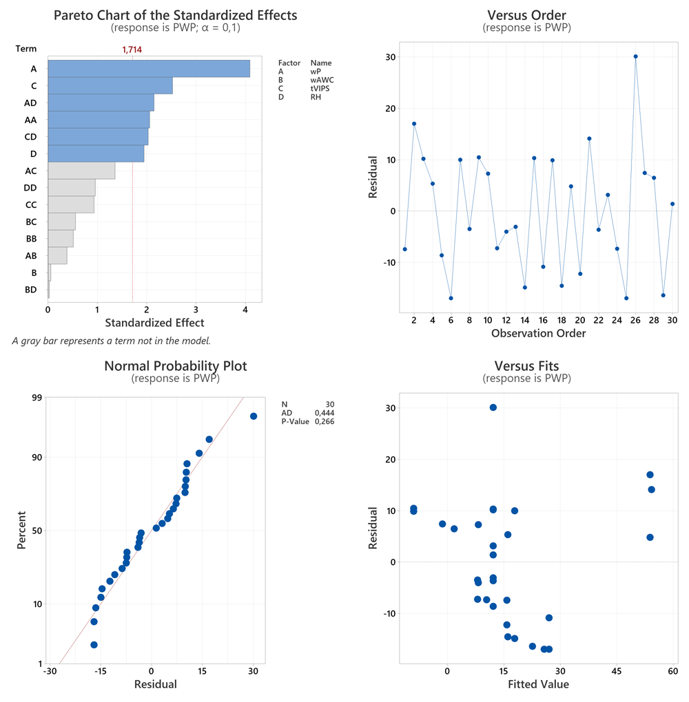
Figure 2. Effects and residual plots for PWP model.
The LEP model explains 31.78% of the variance with linear terms, namely tVIPS (20.59%) and wP (11.18%), and 10.16% with a square tVIPS term. These sources represent the significant effects (Figure 3 (a)). The validity and reliability of the model are sufficient according to Figure 3 (b) – (d). The model fit is 42.4%, but the main error due to Lack-of-Fit is not statistically significant with a p-value of 0.829, as summarized in Table 8. Figure 6 (b) plots the LEP model as a function of factor levels.
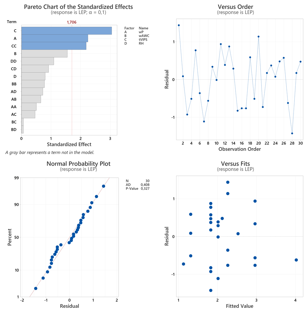
Figure 3. Effects and residual plots for LEP model.
Table 8. ANOVA of LEP model.
| Source | DF | Seq SS | Contribution / % | Adj SS | Adj MS | F-Value | P-Value |
|---|
| Model | 3 | 11.143 | 42.38 | 11.143 | 3.7142 | 6.37 | 0.002 |
| Linear | 2 | 8.355 | 31.78 | 8.355 | 4.1775 | 7.17 | 0.003 |
| wP | 1 | 2.940 | 11.18 | 2.940 | 2.9400 | 5.05 | 0.033 |
| tVIPS | 1 | 5.415 | 20.59 | 5.415 | 5.4150 | 9.29 | 0.005 |
| Square | 1 | 2.788 | 10.60 | 2.788 | 2.7876 | 4.78 | 0.038 |
| tVIPS*tVIPS | 1 | 2.788 | 10.60 | 2.788 | 2.7876 | 4.78 | 0.038 |
| Error | 26 | 15.151 | 57.62 | 15.151 | 0.5827 | | |
| Lack-of-Fit | 23 | 12.241 | 46.56 | 12.241 | 0.5322 | 0.55 | 0.829 |
| Pure Error | 3 | 2.910 | 11.07 | 2.910 | 0.9700 | | |
| Total | 29 | 26.294 | 100.00 | | | | |
| Std. Dev | 0.76 | | | | | | |
| PRESS | 21.1 | | | | | | |
| R² | 0.424 | | | | | | |
| Adj R² | 0.357 | | | | | | |
| Pred R² | 0.199 | | | | | | |
The MD flux model includes three quadratic terms, namely wHC6*wHC6 (23.0%), tVIPS*tVIPS (16.84%), and wP*wP (7.63%). The quadratic terms all show significant effect sizes (Figure 4 (a)). This suggests an optimum of MD performance for intermediate factor levels, as shown in Figure 6 (c), to which all factors contribute significantly. Another source of statistically significant variance is a block term with a contribution of 14.45%. The residual analysis is unremarkable (Figure 4 (b) - (d)). The model fits the data to 61.9% and the Lack-of-Fit error is statistically significant with a p-value of 0.031, concluding that the model does not correctly specify the relationship between response and predictor (Table 9).
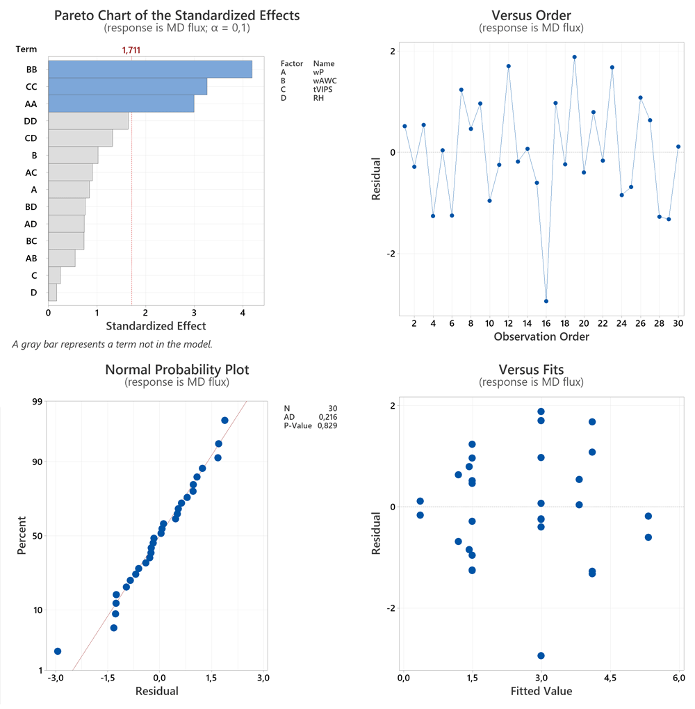
Figure 4. Effects and residual plots for MD flux model.
Table 9. ANOVA of MD flux model.
| Source | DF | Seq SS | Contribution / % | Adj SS | Adj MS | F-Value | P-Value |
|---|
| Model | 5 | 54.7262 | 61.93 | 54.7262 | 10.9452 | 7.81 | 0.000 |
| Blocks | 2 | 12.7708 | 14.45 | 12.7708 | 6.3854 | 4.55 | 0.021 |
| Square | 3 | 41.9553 | 47.48 | 41.9553 | 13.9851 | 9.98 | 0.000 |
| wP*wP | 1 | 6.7454 | 7.63 | 12.5324 | 12.5324 | 8.94 | 0.006 |
| wHC6*wHC6 | 1 | 20.3288 | 23.00 | 24.5578 | 24.5578 | 17.52 | 0.000 |
| tVIPS*tVIPS | 1 | 14.8811 | 16.84 | 14.8811 | 14.8811 | 10.61 | 0.003 |
| Error | 24 | 33.6460 | 38.07 | 33.6460 | 1.4019 | | |
| Lack-of-Fit | 21 | 33.2528 | 37.63 | 33.2528 | 1.5835 | 12.08 | 0.031 |
| Pure Error | 3 | 0.3932 | 0.44 | 0.3932 | 0.1311 | | |
| Total | 29 | 88.3721 | 100.00 | | | | |
| Std. Dev | 1.18 | | | | | | |
| PRESS | 49.4 | | | | | | |
| R² | 0.619 | | | | | | |
| Adj R² | 0.540 | | | | | | |
| Pred R² | 0.441 | | | | | | |
The ANOVA of the salt rejection model in Table 10 suggests only square wP (29.93%) as a source of variation with a significant effect size (Figure 5 (a)), suggesting an optimal factor level within the factor space examined. Furthermore, a block contribution of 15.59% with a p value of 0.038 suggests a change in response due to different conditions between runs. The residuals vs. run plot in Figure 5 (b) shows several severe outliers, which are further confirmed by Figure 5 (c) & (d). The pattern suggests a violation of the model assumptions proposed in the section “Model building and statistical analysis”. Salt rejection was consistently 99.9%, except for a few runs where it was <10%. This suggests defective membranes as a source of poor rejection. The RSM is not suitable for modelling this type of behavior.
Table 10. ANOVA of Salt rejection model.
| Source | DF | Seq SS | Contribution / % | Adj SS | Adj MS | F-Value | P-Value |
|---|
| Model | 3 | 12149.1 | 45.53 | 12149.1 | 4049.68 | 7.24 | 0.001 |
| Blocks | 2 | 4161.0 | 15.59 | 4161.0 | 2080.52 | 3.72 | 0.038 |
| Square | 1 | 7988.0 | 29.93 | 7988.0 | 7988.00 | 14.29 | 0.001 |
| wP*wP | 1 | 7988.0 | 29.93 | 7988.0 | 7988.00 | 14.29 | 0.001 |
| Error | 26 | 14536.6 | 54.47 | 14536.6 | 559.10 | | |
| Lack-of-Fit | 23 | 14536.6 | 54.47 | 14536.6 | 632.02 | * | * |
| Pure Error | 3 | 0.0 | 0.00 | 0.0 | 0.00 | | |
| Total | 29 | 26685.6 | 100.00 | | | | |
| Std. Dev | 23.65 | | | | | | |
| PRESS | 18569.9 | | | | | | |
| R² | 0.455 | | | | | | |
| Adj R² | 0.392 | | | | | | |
| Pred R² | 0.304 | | | | | | |
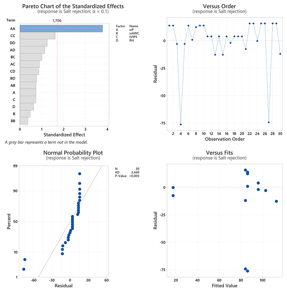
Figure 5. Effects and residual plots for Salt rejection model.
The results of the ANOVA and residual analysis of the four regression models are summarized in Figure 6 and Table 11. Each model is plotted as a function of the four experimental factors. The predictors are on the x-axis and the responses are on the y-axis. The gray shaded plots indicate the absence of statistically significant relationships between predictor and response. The PWP shown in Figure 6 (a) improves with decreasing wP, which is expected as porosity increases. The lack of relationship between PWP performance and HC6 content is puzzling, but a potential effect may be buried in the noise of the data. This is investigated in the section “Results of Multiple Response-Optimization”. In addition, PWP increases linearly with increasing tVIPS and RH. The hypothesis that longer tVIPS at higher RH promotes delayed demixing leading to skin defects will be tested in the section “Morphological analysis”. The plots in Figure 6 (b) show an increasing LEP with increasing wP and decreasing tVIPS. This behavior is reasonable as both actions promote skin densification. HC6 has no statistically significant effect on LEP. At first glance, no effect would be expected as LEP is mainly dependent on the porosity and pore size of the skin. However, the possible effects of HC6 on membrane morphology are discussed in the section “Morphological analysis”. The dependence of LEP on RH cannot be modelled due to the step response between 70% and 75% RH. The MD flux regression model in Figure 6 (c) shows optimal flux for intermediate factor levels of wP, wAWC and tVIPS. This suggests good specified factor level ranges. RH appears to have an inconsistent effect on MD flux. In the case of salt rejection, no statistically significant relationships are expected due to the inadequacy of the RSM to fit the data, see Figure 6 (d).
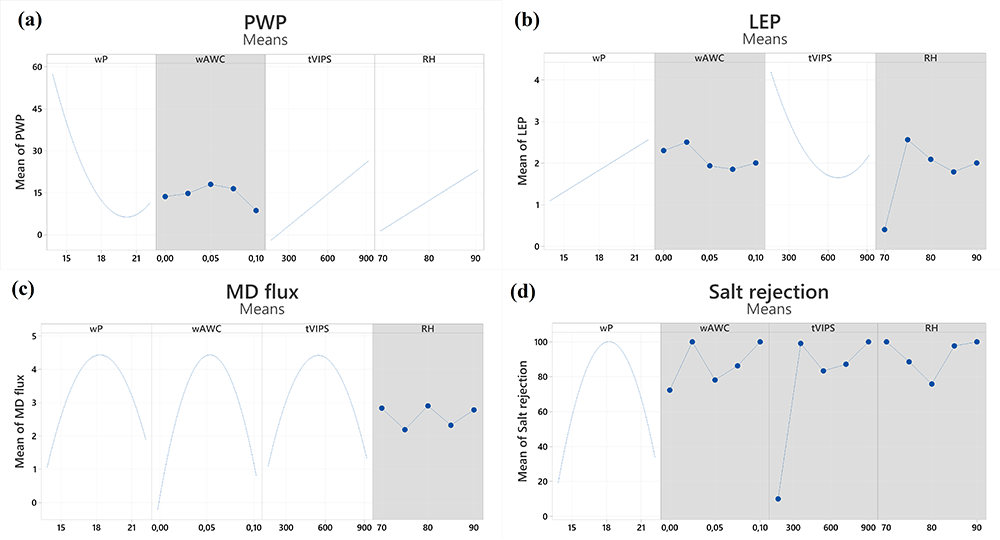
Figure 6. Factorial plots for models.
Table 11. Comparison of model fit.
| Model | PWP | LEP | MD flux | Salt rejection |
|---|
| Lack-of-Fit | insignificant | insignificant | significant | significant |
| Adj R² | 0.539 | 0.357 | 0.540 | 0.3924 |
According to Table 11, the models for MD flux and salt rejection have statistically significant Lack-of-Fit errors, meaning that these models do not correctly specify the relationship between response and predictors. A likely cause could be that the experiment contained an uncontrolled predictor variable. This proposition is supported by the fact that the ANOVA of both models shows statistically significant contributions of blocks as a source of variance. The Lack-of-Fit is not statistically significant for the remaining models, namely PWP and LEP. Overall, the adjusted coefficient of determination is below our expectations. Due to the inadequacy of the RSM model to fit the Salt rejection data it is excluded from further investigation and verification.
Results of Multiple Response-Optimization
To test the predictive capabilities of the remaining three models and to elucidate the effect of HC6 on membrane performance, two multiple response-optimized (MRO) membranes were prepared. Each was part of a set of four additional membranes prepared at the MRO predicted factor levels, but with varying HC6 weight fractions. Finally, both sets consisted of one pure PVDF membrane and four PVDF/HC6 hybrid membranes with 0.025, 0.05, 0.075, and 0.1 wt. % HC6, respectively. The performance of the membranes was evaluated as described in the section “Membrane characterization”.
The first MRO was fitted using the PWP and LEP model. The objective was to maximize PWP while LEP was set at a target of 2.0 bar, which is suitable for MD application. The MRO recommends factor levels to achieve the selected response targets. Table 12 summarizes the experimental parameters of the first MRO membrane set.
Table 12. Dope solution compositions and VIPS conditions of first MRO set.
| Membrane | PVDF / wt.-% | HC6 / wt.-% | DMAc / wt.-% | Exposure time / s | RH / % |
|---|
| M-T0* | 17.3 | 0 | 82.700 | 900 | 90 |
| M-T1 | 17.3 | 0.025 | 82.675 | 900 | 90 |
| M-T2 | 17.3 | 0.050 | 82.650 | 900 | 90 |
| M-T3 | 17.3 | 0.075 | 82.625 | 900 | 90 |
| M-T4 | 17.3 | 0.100 | 82.600 | 900 | 90 |
These results, along with the Standard Error (SE Fit), 95% Confidence Interval (95% CI), and 95% Prediction Interval (95% PI) of the fitted target values are shown in Table 13. The Standard Error of the Fit (SE Fit) estimates the variation in the estimated mean response for the specified factor levels. The Confidence Interval (CI) provides a range of likely values for the mean response given the specified factor levels. The Prediction Interval (PI) is a range that is likely to contain a single response for the specified factor levels.
Table 13. First MRO predictions.
| Factor | Level | |
|---|
| wP / wt.-% | 17.3 | |
| tVIPS / s | 900 | |
| RH / % | 90 | |
| Response | Target | SE Fit | 95% CI | 95% PI |
|---|
| PWP / Lm-2h-1bar-1 | 72.1 | 15.6 | 39.8 – 104.3 | 29.9 – 114.2 |
| LEP / bar | 2.0 | 0.6 | 0.8 – 3.2 | 0.1 – 4.0 |
Table 14 summarizes the membrane performance of the first MRO set. Green underlay indicates values within the 95% CI, orange within the 95% PI. This indicates that the predictive capabilities of the PWP and LEP models are within useful limits, although the MRO overpredicted membrane performance in both cases. An increase in PWP and MD flux performance was reported for all PVDF/HC6 hybrid membranes compared to the pure PVDF membrane, while LEP was also improved. In addition, Salt rejection remained consistently high at 99%. These results confirm the efficacy of HC6 as an agent to improve membrane flux without compromising selectivity or membrane wetting resistance.
Table 14. First MRO results.
| Membrane | LEP / bar | PWP /
Lm-2h-1bar-1 | MD flux / Lm-2h-1 | Salt rejection / % |
|---|
| M-T0* | 1.3 | 35.4 | 5.2 | 99.9 |
| M-T1 | 1.7 | 39.7 | 5.6 | 99.9 |
| M-T2 | 1.6 | 66.8 | 6.2 | 99.9 |
| M-T3 | 1.8 | 47.4 | 8.3 | 99.9 |
| M-T4 | 1.9 | 113.6 | 6.4 | 99.9 |
For the second MRO, both MD flux and PWP were maximized. The required factor levels and fitted response targets, including estimated errors and 95% intervals, are shown in Table 15.
Table 15. Second MRO predictions.
| Factor | Level | |
|---|
| wP / wt.-% | 15.6 | |
| wHC6 / wt.-% | 0.051 | |
| tVIPS / s | 638 | |
| Response | Target | SE Fit | 95% CI | 95% PI |
|---|
| MD flux / Lm-2h-1 | 3.2 | 0.3 | 2.6 – 4.0 | 0.7 – 5.8 |
| PWP / Lm-2h-1bar-1 | 70.5 | 11.1 | 47.6 – 93.4 | 35.0 – 106.0 |
Table 16 summarizes the experimental conditions of the second MRO membrane set.
Table 16. Dope solution compositions and VIPS conditions of second MRO set.
| Membrane code | PVDF / wt.-% | HC6 / wt.-% | DMAc / wt.-% | Exposure time / s | RH / % |
|---|
| M-T5 | 15.6 | 0 | 84.400 | 638 | 90 |
| M-T6 | 15.6 | 0.025 | 84.375 | 638 | 90 |
| M-T7* | 15.6 | 0.051 | 84.350 | 638 | 90 |
| M-T8 | 15.6 | 0.075 | 84.325 | 638 | 90 |
| M-T9 | 15.6 | 0.100 | 84.300 | 638 | 90 |
Table 17 summarizes the membrane performance of the second MRO set. The PWP is within the 95% CI, further confirming the predictive ability of the model. The MD flux performance as a function of HC6 concentration qualitatively agrees exactly with the model prediction, although the model underpredicts the membrane performance to an extent outside the 95% PI. This suggests that the MD flux model is only qualitatively suitable for predicting membrane MD performance. Both PWP and MD flux are improved for the PVDF/HC6 hybrid membranes over the pure PVDF membrane, except for the MD flux of M-T9. LEP and Salt rejection are lower compared to the first MRO, possibly due to reduced polymer content, which increases porosity.
Table 17. Second MRO results.
| Membrane | LEP / bar | PWP /
Lm-2h-1bar-1 | MD flux / Lm-2h-1 | Salt rejection / % |
|---|
| M-T5 | 1.5 | 62.5 | 5.2 | 99.9 |
| M-T6 | 1.5 | 81.6 | 5.3 | 98.43 |
| M-T7* | 1.3 | 91.8 | 7.9 | 87.89 |
| M-T8 | 1.3 | 67.8 | 6.0 | 98.12 |
| M-T9 | 1.4 | 73.4 | 4.3 | 80.5 |
The multiple response optimization was a twofold success. On the one hand, the combined DoE and MRO approach resulted in membranes with a performance improvement that clearly exceeded the benchmark of the best performing CCCD membranes. Compared to these membranes, the performance improvement was 7.0 times for PWP (M-T4) and 3.3 times for MD flux (M-T3). In addition, a comparison of pure PVDF and PVDF/HC6 hybrid membranes within each MRO set shows the improved performance of the hybrid membranes. The first MRO set maximized PWP and targeted an LEP of 2.0 bar. The pure PVDF membrane M-T0 showed a PWP of 35.4 Lm-2h-1bar-1 and an LEP of 1.3 bar. The best performing hybrid membrane, M T4, measured 113.6 Lm-2h-1bar-1 with an LEP of 1.9 bar. In addition, MD flux improved from 5.2 Lm-2h-1 to 8.3 Lm-2h-1 for M-T3 over M-T0. This represents a 3.2-fold increase in PWP and a 1.6-fold increase in MD flux. MD selectivity remained high for both hybrid membranes with a salt rejection of 99.99%. The second MRO was optimized to maximize MD flux and PWP. The pure PVDF membrane M-T5 showed an MD flux of 5.2 Lm-2h-1 and a PWP flux of 62.5 Lm-2h-1bar-1. The best performing hybrid membrane, M-T7, showed an MD flux of 7.9 Lm-2h-1 and a PWP of 91.8 Lm-2h-1bar-1, representing a 1.5-fold increase in MD and PWP performance. On the other hand, three out of four regression models, namely LEP, PWP and MD flux, were validated despite the mediocre Adj R².
Morphological analysis
SEM was used to study the morphological analysis of the two sets of MRO membranes. The first MRO, maximized PWP while targeting a LEP of 2.0 bar. The PWP and MD flux of the PVDF/HC6 hybrid membranes increased compared to the pure PVDF reference membrane. This could be explained by the presence of the AWC within the polymer matrix, as shown by the SEM micrographs of the top surfaces and cross-sections of the prepared membranes. We suggest that the incorporation of the HC6 molecules could have ruptured the skin during membrane formation without staying in the polymeric matrix (Nursiah et al., 2023), which is also reminiscent of the role of LiCl as a pore forming agent during the preparation of PVDF membranes (Tomaszewska, 1996). The top surface of the pure PVDF membrane (Figure 7 (a)) shows a dense skin layer, whereas the surfaces of the PVDF/HC6 hybrid membranes show a gradual increase in porosity with increasing HC6 content (Figure 7 (b)–(e)). The incorporation of the AWC also seems to induce a higher volume of voids and cavities throughout the membrane cross-sections, as indicated by the evolution of the finger-like voids in the reference membrane (Figure 7 (f)) into deeper and larger voids in the hybrid membrane cross-sections (Figure 7 (g)–(j)). This shift in the morphological structures of the PVDF/HC6 hybrid membranes is similar to that seen in our previous publication using NIPS (Nursiah et al., 2023).
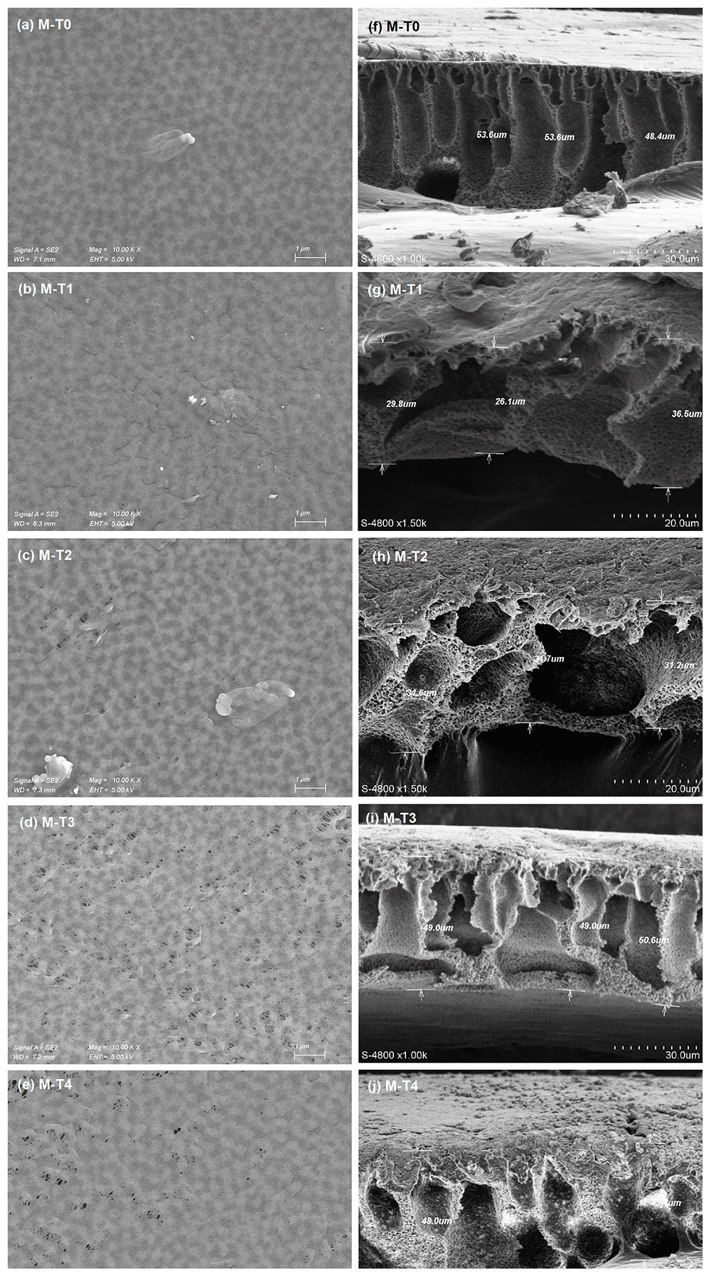
Figure 7. SEM micrographs of top surfaces and cross-sections of the first MRO membranes.
(a)-(e): Top surfaces; (f)-(j): Cross-sections.
The second MRO maximized both PWP and MD flux. All PVDF/HC6 hybrid membranes showed improved PWP and MD flux performance compared to the pure PVDF membrane, similar to the first MRO. A comparison of the surface morphologies of both MRO membrane sets clearly shows a higher degree of surface porosity for the second set Figure 8 (a)–(e). Even the pure PVDF membrane MT-5 has micropores, while MT-0 has a flawless skin. The upper surfaces of the PVDF/HC6 hybrid membranes clearly show increased porosity compared to the pure PVDF membrane M-T5. The surface pores of the hybrid membranes appear to be somewhat stretched as shown in Figure 8 (c)–(e). This observation may explain the lower LEP and Salt rejection compared to M-T5 and M-T6. The average LEP and Salt rejection of the first set is 1.7 bar and 99.9%, while the second set is 1.4 bar and 93.0%. The combined effects of lower polymer content, shorter tVIPS and HC6, increase the surface porosity to a level that provides the best MD performance in this study. However, this extreme level of surface porosity facilitates membrane wetting as evidenced by decreased LEP and salt rejection. Furthermore, the cross-sections of the membranes are found to be denser than that of the reference membrane M-T5, in contrast to the asymmetric structures with deep finger cavities observed in the first MRO. Nonetheless, the SEM micrographs of the top surfaces of the PVDF/HC6 hybrid membranes in Figure 8 provide further evidence of the effect of AWC within the polymeric matrices.
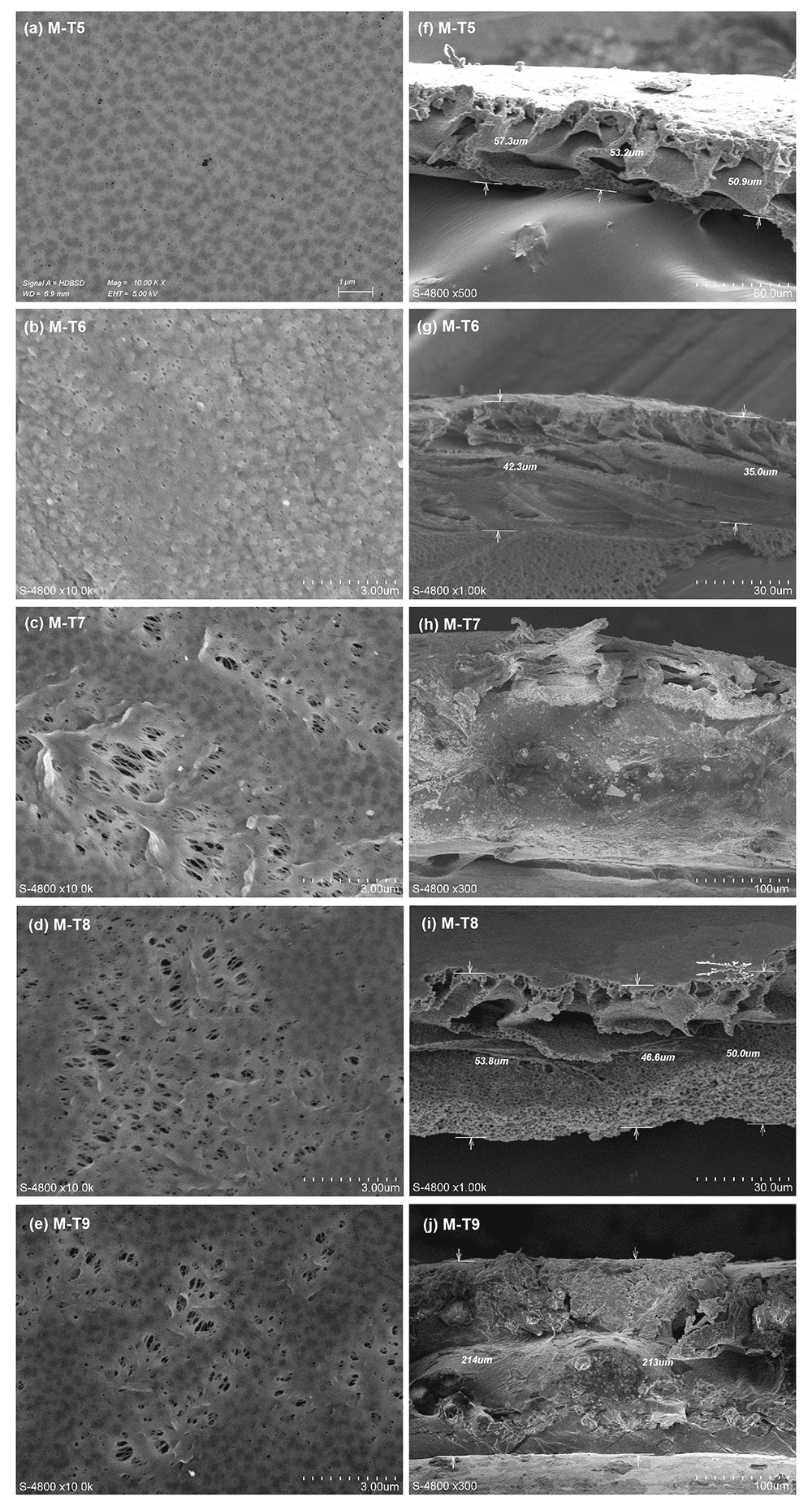
Figure 8. SEM micrographs of top surfaces and cross-sections of the second MRO membranes.
(a)-(e): Top surfaces; (f)-(j): Cross-sections.
From the morphological analysis of the MRO membrane sets three conclusions can be drawn.
a) A combined VIPS-NIPS process was used to better tailor the morphological and mechanical properties of the membranes for MD. The asymmetric membrane structures indicate that the VIPS step alone did not achieve complete phase inversion throughout the cross-section. The asymmetric cross-sections suggest that the NIPS step completed the phase inversion process. The mechanical properties of the membranes were sufficient, as all samples withstood 4.0 bar for 45 min during the LEP measurement.
b) The morphology of the cross-sections of the hybrid PVDF/HC6 membranes further confirms the mechanism of incorporation of the AWC into the PVDF matrix as explained in the previous work (Nursiah et al., 2023). The high affinity of the amphiphilic imidazole head of the HC6 molecule for water increases the mass transfer rates during the NIPS phase of the precipitation process. This results in larger macrovoids in the sublayer. Therefore, it is suggested that instantaneous demixing is preferred over delayed demixing during the VIPS-NIPS process.
c) At the same time, however, HC6 increases surface porosity during the VIPS stage of the VIPS-NIPS process. We propose that the slower non-solvent mass transfer rate during VIPS allows the formation of AWC crystals within the dope before phase separation occurs, thereby disrupting skin formation during the NIPS stage. Therefore, the VIPS stage did not produce the desired bi-continuous surface structure, but surface porosity was still achieved by the presence of HC6. These results show that HC6 favors the formation of asymmetric cross-sections, independent of the phase inversion process.
Conclusion
The scope of this work was to investigate the potential benefits of combining AWC and VIPS to enhance MD performance in PVDF membranes. A combined DoE and RSM approach was used to evaluate the interactions between the experimental parameters, namely polymer content, HC6 content, VIPS duration and RH, with the aim of optimizing membrane performance as specified by MRO.
Based on the performance of the prepared membranes, four regression models were derived, namely PWP, LEP, MD flux and salt rejection. ANOVA of these models suggests that PWP and LEP models correctly specified the relationship between response and predictors, while the MD flux and Salt rejection models did not, due to statistically significant Lack-of-Fit errors. Experimental verification of the models by MRO confirmed that the PWP and LEP models predict membrane performance with reasonable confidence. The MD flux model qualitatively accurately predicts membrane performance, but quantitatively underpredicts it. Thus, three out of four regression models were validated despite a mediocre Adj R². Two sets of MRO membranes with different HC6 content confirmed that AWC improves PWP and MD flux without sacrificing LEP or selectivity. Morphological analysis by SEM revealed an increase in the skin porosity of the hybrid membranes, although the skin did not disappear completely by incorporating a VIPS stage. However, the asymmetric cross-sections with finger-like structures of the first MRO set confirmed the proposed mechanism for the incorporation of AWC into the PVDF matrix (Nursiah et al., 2023). These results tend to indicate that the use of AWC as an additive in membrane preparation by VIPS and NIPS will favor the formation of asymmetric cross-sections. However, this effect has only been demonstrated using water as a non-solvent, which has a strong affinity for the amphiphilic part of HC6.
Ethics and consent
Ethical approval and consent were not required.