Morphing 2 mObjects
The examples below details the interpolation of recordings of a male speaker and a female speaker uttering the same word from an excellent database of American English Vowels (Hillenbrand et al., 1995) but can be applied to any other pair of mObjects such as recordings of different emotional expressions from the same speaker.
○ Generating the average of two mObjects
To generate an average of the mObject1 (Figure 2A) and mObject2 (Figure 2C), a rate of 0.5 is set for each mObject, such that each the 5 mRates fields equals [0.5 0.5]. Running VoiceMultiMorph generates the new mObjectM which can then be synthesized, listened to, saved if necessary and inspected. Figure 2b shows the smoothed spectrogram of the 2-voice average. Note that since the Frequency anchors of the two original mObjects in this example correspond to frequencies of their first 3 formants, the Frequency anchors of the newly generated mObjectM also provide its 3 formant frequencies.
To generate a continuum between the two sounds, variable rates are set using a parameter k: mRates=[k 1-k], with k between 0 and 1. k represents the weight of the first mObject, such that a value of k=1 (mRates=[1 0]) corresponds to the first mObject, a value of k=0 (mRates=[0 1]) corresponds to the second mObject, and values between 0 and 1 to interpolation between the 2 mObjects. Parameter k can be set at regular intervals between 0 and 1 to generate a series of mObjects regularly spaced between the 2 original mObjects. For instance k=[1:-0.1:0] will generate a series of 11 mObjects in 10% steps between the two original mObjects. Or k=[0.95:-0.15:0.05] will generate 7 mObjects in 15 % steps between a 95%/5% and a 5%/95% morphs – such that each sound of the continuum contains some part of the two original sounds (Figure 2D).
Such continua are particularly interesting as they provide series of stimuli with equal acoustical distance between any two consecutive stimuli and can thus be used to dissociate perceptual aspects of a particular voice dimension (here, gender) from the unavoidable physical differences between the stimuli. For instance, the same 15% acoustical difference between 2 consecutive gender morphs has very different perceptual effects depending on whether they are towards the extremes of the continuum, or towards the middle of the continuum where it leads to marked changes in perceived gender (Charest et al., 2013; Pernet & Belin, 2012).
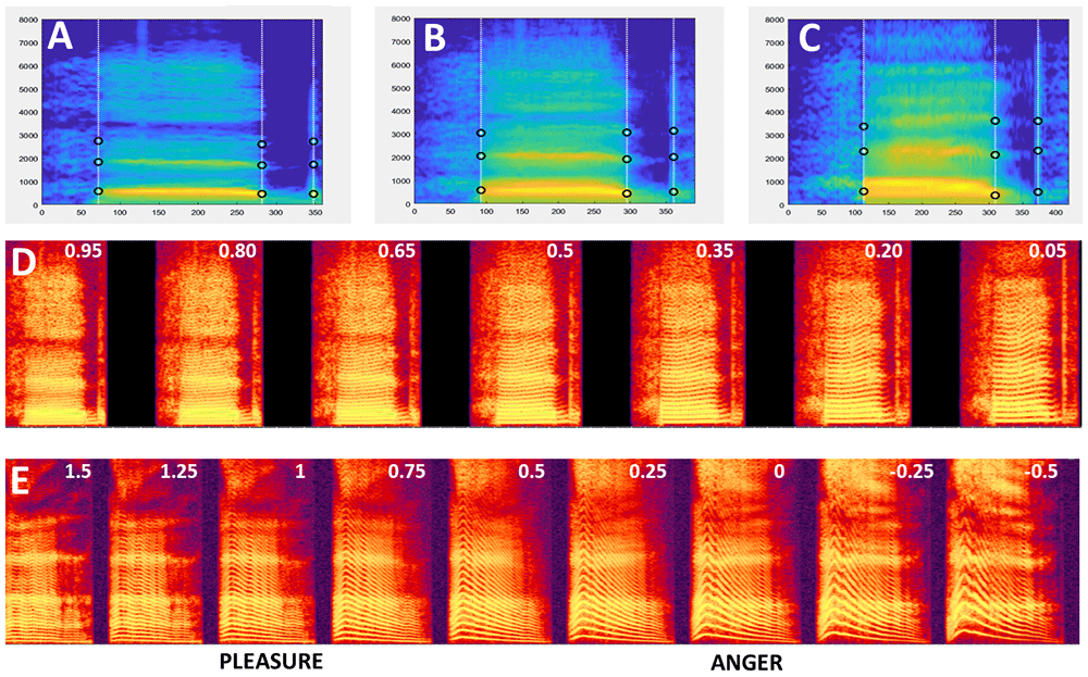
Figure 2. Morphing 2 stimuli.
A–C. Smoothed spectrograms with Time and Frequency anchors of 3 mObjects. A: M48eh. C: W33eh. Note the similar definition of Time and Frequency anchors. B: Average of M48eh and W33eh. D. Spectrogram of the continuum generated between M48eh and W33eh using values of k =[0.95:-0.15:0.05] . Values of k are indicated at the top of each spectrogram. The leftmost stimulus is a 95%/5% mix of M48eh and W33eh, decreasing/increasing in steps of 15% until the rightmost stimulus – 5%/95% M48eh and 95% W33eh. The middle stimulus is the 50%/50% average shown in B. Any pair of consecutive stimuli is separated by the same acoustical distance at any point of the continuum: 15% of the M48eh-W33eh distance. E. Pleasure-Anger continuum including caricatures generated using values of k=[1.5:-.25:-0.5].
In the continuum example of Figure 2D mRates kept values between 0 and 1, which makes intuitive sense but is not mathematically required. Indeed, while mRates values between 0 and 1 correspond to stimuli generated between mObject1 and mObject2 in the line between the two in multidimensional voice space, values below 0 and above 1 correspond to points beyond the two mObjects on that same line; i.e., caricatures (Calder et al., 2000; Whiting et al., 2020).
For instance, mRates = [1.5 -0.5] correspond to a point on the line at 50% of the mObject1-mObject2 distance on the side of mObject1 – in the example above, a voice exaggerating gender difference towards the male voice – while mRates=[-0.5 1.5] will produce and exaggeration of the same magnitude but towards the female voice. So by using mRates=[k 1-k] and k extending beyond 0 and 1 the continuum will be extended on both sides with increasingly strong caricatures. Figure 2E shows the spectrogram of an emotion continuum generated using k=[1.5:-0.1:-0.5] between a pleasure (6_pleasure.wav) and an angry (6_anger.wav) expression from an actor of the Montreal Affective Voices (Belin et al., 2008). Note that using mRates values too negative or too much above 1 will likely result in unnatural sounding stimuli...
In the examples above all 5 fields of the mRates structure were set to the same values. But it can be desirable in some cases to set some fields to different values than other, what has been called ‘parameter-specific morphing’ (Skuk et al., 2020). For instance, all stimuli of the continuum could be set to the same duration – the average duration of mObjects 1 and 2 – by using mRates.duration=[0.5 0.5] while mRates in the other fields vary with k. Or, the anchorFrequency field could be set to [0.5 0.5] while the others vary with k, to generate a continuum of stimuli all having the formant frequencies of the mObject1-mObject2 average.
Morphing N mObjects A significant feature of VoiceMultiMorph is that it treats morphing N>2 mObjects in exactly the same way as for 2 mObjects. Simply, there are N dimensions instead of 2 to the multidimensional voice space defined by the mObjects, and mRates fields consist of a vector of N values (still adding up to 1 for each field) that can be viewed as the coordinates of the new mObjectM in N-dimensional voice space. Rather than averaging in turn all stimuli in successive steps, the user simply defines the desired coordinates in that space, and performs a single generation of mObjectM and resynthesis no matter how many stimuli are combined. In the examples below we consider 16 mObjects generated from recordings of the word ‘Hello’ spoken by 16 female speakers (Figure 3A) as part of a study on voice personality impressions (McAleer et al., 2014). The first step consists in loading the 16 mObjects in a cell array of structures.
As for 2 mObjects, to generate the average of N mObjects the mRates vectors are all set to the same value of 1/N, here mRates=[1/16 … 1/16] or ones(1,16)/16. The mObjectM generated by these mRates values can be viewed as the center of N-dimensional voice space. It has average f0 contour and duration; it has average aperiodicity map, resulting in a very smooth spectrogram (Figure 3B) with high harmonics-to-noise ratio. Such an average stimulus is typically perceived as more attractive than individual voices (Bruckert et al., 2010) and elicits lower activity in the TVAs than individual voices (Bestelmeyer et al., 2011; Latinus et al., 2013)– potentially reflecting a norm-based coding mechanism relative to an internal prototype.
It can be interesting to interpolate between a single mObject and the N-Average: studies in the face perception domain use this strategy to modulate the ‘identity strength’ of the faces (Leopold et al., 2001). To do so, one strategy could be to first generate the mObject corresponding to the N-Average, then generate the continuum between the 2 mObjects as in the example above. Another, better strategy, that skips an unnecessary step, is to specify directly the mRates of the desired continuum trajectory in N-dimensional space.
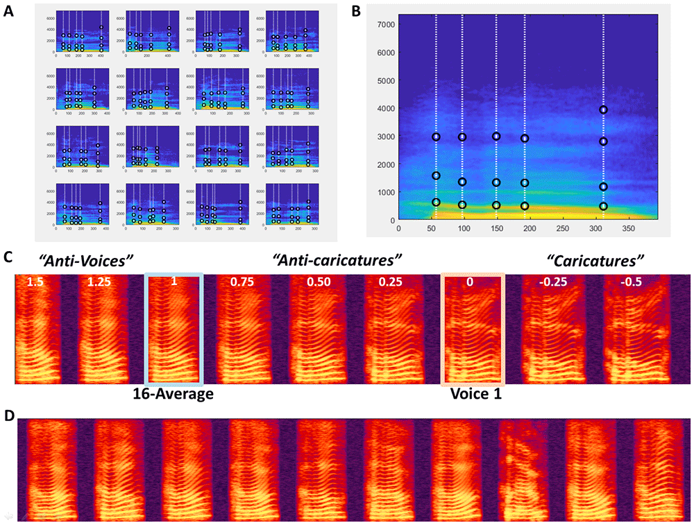
Figure 3. Morphing 16 mObjects.
A. 16 mObjects of the word Hello spoken by 16 female speakers. Note their similar definition of the Time and Frequency anchors for combined morphing. B. MObjectM corresponding to the average of the 16 mObjects. C. Spectrogram of Continuum between Voice1 and the 16-Average with negative values of k for Caricatures and values of k greater than 1 for ‘Antivoices’ (Latinus & Belin, 2011). D. 10 random ‘Hellos’ generated using random mRates.
With k=[1.5:-0.1:-0.5] as in the example above, to interpolate between the N-Average and mObject1, using mRates = [k*ones(1,16)/16] + [(1-k)*[1 zeros(1,15)]] or ([1-k+k/16 k/16 k/16… k/16] will generate stimuli on the line in multidimensional space going through mObject1 and the N-Average. K=1 corresponds to the average; k=0 to mObject 1. Values of k between 0 and 1 correspond to stimuli between the N-Average and mObject1 (‘anti-caricatures’); values of k below 0 correspond to caricatures of mObject1 relative to the average. Values of k above 1 correspond to ‘anti-voices’, i.e. stimuli on the other side of the average relative to mObject1 in voice space, with opposite characteristics, e.g., higher than average f0 if mObject1 has lower f0 than average, etc. (Figure 3C)
Generating continua with the N-average can also be used for instance to take advantage of its high harmonics-to-noise ratio and generate ‘smoother’ or ‘rougher’ versions of mObjects. By using mRates values of [1 0 0 … 0] for all mRates fields, except for mRates.aperiodicity=[k*ones(1,16)/16] + [(1-k)*[1 zeros(1,15)]] stimuli will keep all aspects of mObject 1 but for the degree of aperiodic noise, and moving it closer to the average will generate a version of mObject1 with less aperiodicity, which listeners find more attractive (Bruckert et al., 2010)
The N mObjects can be viewed as the axes of an N-dimensional voice space they define. While all points of that space likely do not correspond to naturalistic voice stimuli – depending of course on the choice of the N mObjects – many points in the region around the average likely do. The N mObjects thus constitute a generative space that can be used to synthesize any point of the space. By applying random weights to each mObject in the mRates (still ensuring the total adds up to 1 per field), it is possible to sample the voice space by generating an arbitrary number of random stimuli. The example in the STRAIGHTMORPH_tutorial.m script applies random weights, with a coefficient that modulates the radius of the hypersphere around the average in which stimuli are generated, in order to generate an arbitrary number of random ‘Hellos’ and keeps the same weights across the 5 fields of the mRates.