1. Introduction
In modern industrial systems, data has become an integral part of the production process, with a vast amount of information being generated daily, through sensors during the production, or even via human input during process control. A sufficient amount of data has been proven to boost, among others, the hypothesis generation and increase the accuracy of the desired results1. Nevertheless, the generated industrial data are often complex and noisy, which makes the identification of anomalous behaviors (e.g. equipment failures) a difficult task.
Anomaly detection (AD) methods can help in the identification of such defective parts, minimizing the risk of costly downtime and safety issues. Particular examples of the importance of anomaly detection, highlighting the emergence need of effective methods in this field of study, regard healthcare2 and transportation industry3, where any malfunction can lead to fatal results. Both supervised and unsupervised techniques have been attempted by the wider scientific community to address the task of anomaly detection. Specifically, some of the most widely used anomaly detection methods are based on: Nearest Neighbors4–9, Clustering10, Statistics11, Deep Learning12–15, Support Vector Machines16, Bayesian Networks17 and Rule-based anomaly detection18.
In recent years, machine learning applications specifically pertaining to anomaly detection on manufacturing or industrial data, have consolidated their place in this area on account of the high accuracy they provide19. More specifically, Malhotra et al.20 were one of the first that introduced deep learning techniques in AD tasks that can be applied on time series data sets. The Long Short-Term Memory AutoEncoder (LSTM-AE) scheme they proposed for anomaly detection learns to reconstruct ‘normal’ time-series behavior and then uses reconstruction error to detect anomalies. The effectiveness of stacked LSTM networks for anomaly/fault detection in time series is demonstrated using various manufacturing-oriented data sets, with multi-sensor engine data sets among them. The main takeaway from this paper is that LSTM networks can be used for anomaly detection in time series data by learning to reconstruct ‘normal’ time-series behavior and detecting anomalies using reconstruction error through an AutoEncoder network.
Dimitriou et al.21,22 proposed a 3D-Convolutional Neural Network (3DCNN) that outperforms several deep architectures on the estimation of defects in the conductive glue attachment in manufacturing miniature Printed Circuit Boards (PCB). The authors also model the geometric variations in manufacturing parameters and predict upcoming events related to sub-optimal performance. In 23, the authors utilize deep neural networks (DNNs) in metal parts manufacturing. More specifically, they have tried to automate the manufacturing process for the machine condition monitoring and 3D inspection of defective hard metal parts, by using DNNs to investigating the defects on real production samples.
Ergen et al.24 also utilize LSTMs to perform anomaly detection on multi-sensory data streams, by transforming variable length sequences to fixed length windows and then applying One-Class Support Vector Machines (OC-SVM) and Support Vector Data Description (SVDD) algorithms to detect the anomalies. Based on their finding, greatly improved the detection accuracy compared to conventional AD techniques.
Rousopoulou et al.25 presents a cognitive analytics platform for anomaly detection which is capable to handle, analyze and exploit resourcefully machine data from a shop-floor of factory, so as to support the emerging and growing needs of manufacturing industry. The introduced system contributes to industrial digitization and creation of smart factories by providing a generic platform which is a complete solution supporting standards-based factory connectivity, data management, various Artificial Intelligence (AI) models training and comparisons, live predictions and real-time visualizations.
More recently, Zhang et al.14, observing the vast amounts of multivariate time series data that are generated in real-time by Industrial Control Systems (ICS), decided to model the complex temporal correlation of that multi-sensor data. The framework that they introduce is comprised of two main components, a Deep Convolutional AutoEncoders (CAE-M) network to capture the aforementioned correlations as well as a memory network with BiLSTMs and autoregressive models that attend to the spatiotemporal data dependencies. Experimental results indicate that their method outperforms previous works on several manufacturing testing data sets.
Since this is a particularly active research field, contemporary methods and architectures constantly bring something new to the table that improves on some previous findings. It is believed that cutting-edge deep learning techniques such as Anomaly-based transformers as well as progressive (or continual) learning methods may have been overlooked based on the literature, especially when it comes to manufacturing data in time series format. Working towards the goal of more robust anomaly detection on manufacturing data, we explore these methods using our data set. In this study, a comparative analysis of multiple supervised and unsupervised anomaly detection algorithms based on industrial data is performed. The motivation behind our work is to evaluate the performance of state-of-the-art anomaly detection techniques on real, multi-dimensional data. Additionally, the importance of interpretability along with the absence of transparent models is acknowledged, which limits the use of anomaly detection in high-risk scenarios. For this purpose, recent scientific studies are taken under consideration in an attempt to unravel the explainable behavior of the examined models.
Interpretable, or eXplainable Artificial Intelligence (XAI), as a term, is defined as something “you can decide that it has a particular meaning”1. With the increasing use of machine learning algorithms in high-risk industries, including healthcare, criminal justice and anti-discrimination law, the need for transparent predictive models is higher than ever before. The main incentives of explainable machine learning are to justify each decision, to control the model itself, to potentially improve the model and finally to discover new technologies through the help of advanced models26.
Interpretability methods may be further classified according to certain criteria, into three main categories27,28. Intrinsic or post hoc interpretability refers to either transparent models with the ability to explain themselves (self-explained models) or black-box models that require the application of additional methods to extract explanations. Model-specific or model-agnostic interpretability refers to methods that can be applied to just a specific type of model (e.g. Neural Network) or into any type of model, respectively. Moreover, Local or global interpretability regards models that provide a distinct set of explanations about each specific instance of the data, or explanations about the entire behavior of the model. This study focuses on model-specific, post hoc interpretable methods on black-box models.
In this work, two explainability methods are presented to cover the unsupervised and supervised learners. Starting with the latter, the LionForest algorithm is utilized to train a Random Forest model (binary classifier in our case) on a unique task and deliver to the user a concise rule in natural language that is relatively straightforward and simple to comprehend. Concerning the unsupervised transformer models, the turn-key MLW-XAttentIon solution is devised and implemented, using minimal computational overhead that transforms weights to feature importance vectors which can be interpreted similarly to Shapley value plots. This act of utilizing the entire set of trainable weights along with the input instances has not been considered in anomaly detection-oriented transformer networks, however, the experimental results are comparable to those of proven methods (i.e. LionForest) adding to the overall validity and significance of MLW-XAttentIon.
The use of explainable AI methods referred in Section 3.3 and the examination of their role and effectiveness in inference process lead us to two key questions during the evaluation process:
The answers to these main questions, are given after the presentation of the the experimental results of all anomaly detection methods and the final conclusion is drawn.
The remainder of the paper is organized as follows. In Section 2, the problem of anomaly detection in industrial automation along with the dataset that is utilized are described. In Section 3, the anomaly detection methods used in this study, as well as the interpretability techniques are analyzed. In Section 4, the parameter setup of anomaly detection methods and their experimental results are presented, while in Section 5 we draw our conclusions.
This work is supported by Horizon 2020 (H2020) Framework Programme KnowEdge project that proposes several major innovations for Industry 4.0 in the areas of data management, data analytics and knowledge management such as, AI services that allow the usage of edge deployments as computational and live data infrastructure, a digital twin of the shop-floor able to test AI models, privacy and confidentiality, Human-AI Collaboration and Domain Knowledge Fusion tools, standardization mechanisms and a knowledge marketplace platform29,30.
2. Problem definition - dataset description
Anomaly detection commonly refers to the process that entails the identification and isolation of points that do not conform to the norms or patterns of existing data, displaying erroneous characteristics. The added-value benefits of such points are undeniable for any business or corporation seeking to gain better insights into their production line infrastructure.
In the present day, companies adopt anomaly detection mechanisms as part of a larger framework that oversees day-to-day operations, most notably via customized business intelligence systems31.
2.1 Problem definition
The problem that this work addresses entails formulating an anomaly detection pipeline for Kautex Textron GMBH, a company operating in the automotive industry. Naturally, this manufacturing division of this company generates a considerable number of parts (see Figure 1) in its day-to-day operations, thus identifying problematic sections of this process is of great importance from a variety of standpoints. More specifically, the driving forces behind this particular task, pertain to the needs of the company and are multi-fold:
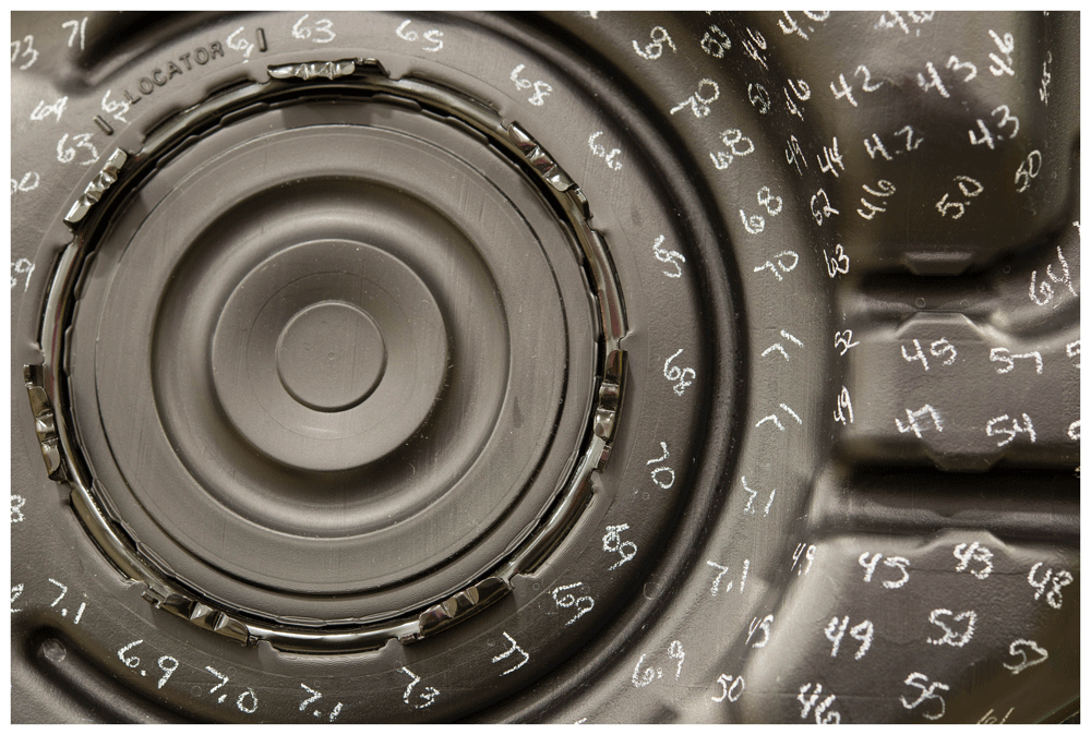
Figure 1. Measuring thickness at different points in final product so as to detect anomalies.
In recent years, the company struggled with significant machine downtime on specific manufacturing posts forced upon the large number of defects that negatively impacted reliability and quality KPIs.
Maintaining a malfunctioning working pipeline increases energy consumption, driving the overall operating costs up, a point that was amplified by the volatile geopolitical landscape.
Working towards cutting-down operating costs, a key problem outlined by the company was the ever-increasing scrap rates that were a result of manufacturing pipelines that performed poorly (relatively large number of defective parts) which could not be detected promptly.
Finally, another crucial problem the company faced, was designing a streamlined production pipeline via the cooperation of humans and machines; that is to incorporate a human-in-the-loop schema where the AIs decisions would be aided by the knowledge provided by domain experts actively engaged in the manufacturing process. The vast amounts of data generated every second by sensors add to the enormous complexity of this task, for any human annotator, thus incorporating automated methods plainly offers an important competitive advantage.
To overcome these challenges, the main goal was to focus on specific components of the manufacturing process and leverage the data provided by Kautex (time series, collected from numerous sensors) to detect anomalies efficiently and accurately. Additionally, labels sourced from experts to gauge the predictive performance of these machine learning methods were utilized.
2.2 Dataset description
Successfully solving a particular task, is highly correlated with the quality of the data provided for each specific case. It is a fact that a large dataset can be particularly advantageous in our field of study, where an attempt to identify defective parts of the production is made. The data utilized in this study were derived from three primary data sources of the company, containing information about every phase of the construction of car parts through a blow molding production line. The three data sources are: the Manufacturing Data (MD) source that refers to information collected during the blow molding procedure of a part, the Computer Aided Quality data (CAQ) source that contains measurements gathered exclusively through online quality inspections right after each part is produced, and Statical Process Control data (SPC) source that refers to measurements gathered through offline quality inspections. Table 1 contains a description about the number of samples, number of features and the date of the first and last recorded instance of each data source.
Table 1. Number of Samples/Features and Start/End recorded dates of each data source.
| #Samples | #Features | Start date | End date |
|---|
| MD | 14266999 | 479 | 10/11/2022 | 19/12/2022 |
| CAQ | 38482 | 13 | 02/11/2022 | 02/01/2023 |
| SPC | 401040 | 11 | 01/12/2022 | 05/01/2023 |
All three data sources contain a unique identifier, which ultimately gives the opportunity to connect them together. The connection between MD and CAQ data can be achieved through their Timestamp feature. Whenever the production of a part is complete, a Timestamp is ascribed and noted on the MD data source and afterwards the same part goes through the inspection phase, where a new Timestamp is noted, this time on the CAQ data source, which has one minute difference with the MD Timestamp. In addition to the Timestamp feature on the CAQ data, a Barcode is also noted, which is used to connect CAQ and SPC data sources, since SPC does not take into consideration the time of the inspection. It is important to mention that due to annotated information provided by the CAQ data source, both supervised and unsupervised machine learning methods can be utilized to solve our task.
Despite the fact that it is possible to connect all data sources into one combined dataset as described above, anomaly detection cannot be applied yet, since each one of the data files may not contain the same amount of features. Additionally, as an attempt to reduce space complexity, the value of each feature is recorded only if it differs from its previously recorded value, otherwise is not recorded at all and should be considered unchanged.
2.2.1 Pre-processing. The successful deployment of machine learning methods requires suitable and credible data, which can be achieved through a pre-processing step. In this work, the pre-processing phase consists of three main components: (a) data cleaning in which the goal was to impute or eliminate instances with missing values or values that do not follow the standard predefined format of that particular feature, (b) feature selection in which multiple feature selection methods are utilized, and (c) data transformation in which, after connecting all data sources through their identifier, any categorical features value is transformed into numerical, with the use of label-encoder2, while missing values are imputed with the forward fill method3.
Specifically, during the feature selection phase, a thorough strategy involving nine separate methodologies was used, as a result of the complicated structure and high-dimensionality of the dataset. The primary objective was not only to remove unnecessary features, but also reduce the complexity of the data to make model training less stressful. Namely, scikit-learn based feature selection methods4, such as VarianceThreshold, SelectKBest, SelectPercentile, Recursive Feature elimination, Recursive Feature Elimination with Cross-Validation along with Forward/Backward selection5, XGBoost importance-based feature selection6 and Correlation matrix were utilized.
The final set of chosen features emerged by combining the most frequently selected features across all aforementioned methods, resulting in a collection of 20 features. Moreover, in order to mitigate redundancy, highly correlated features were subsequently eliminated, further reducing the feature count to 14.
In summary, the main objective is to combine information from several data sources into a unified dataset. Following the completion of the pre-processing stage, a dataset comprising of multiple instances of 14 features gathered between 11/12/2022 and 19/12/2022 was retained. To get a better understanding of the feature attributes found inside the data, Table 2 contains various information regarding a particular feature of the dataset.
Table 2. Characteristics for a particular feature of the dataset after the pre-processing steps.
| Attribute | Value |
|---|
| Distinct | 72 |
| Missing | 0 |
| Infinite | 0 |
| Mean value | 184.36 |
| Minimum value | 0 |
| Maximum value | 203 |
| Zeros value | 0 |
| Negative | 0 |
2.2.2 Cycles. Based on the technical description of the data set, every tank should follow the same predefined production process. This pipeline entails a finite set of processes that must be executed in sequence to ensure the finished result is consistent and also meets certain standards. Manufacturing data, which, to reiterate, are data collected directly from machines, possess a binary feature that dictates the start/end of a machine cycle as illustrated in Figure 2.

Figure 2. Demonstration of two machine cycles.
Ensuring the machine operation is automatic (no human intervention) is a necessary and sufficient condition to support this schema. This condition holds true in this particular case. Naturally, the duration of a cycle is heavily influenced by the tank variant. Fluctuations can also be attributed to other variables such as unforeseen delays or machine failures that cannot be predicted in advance. (Figure 3)
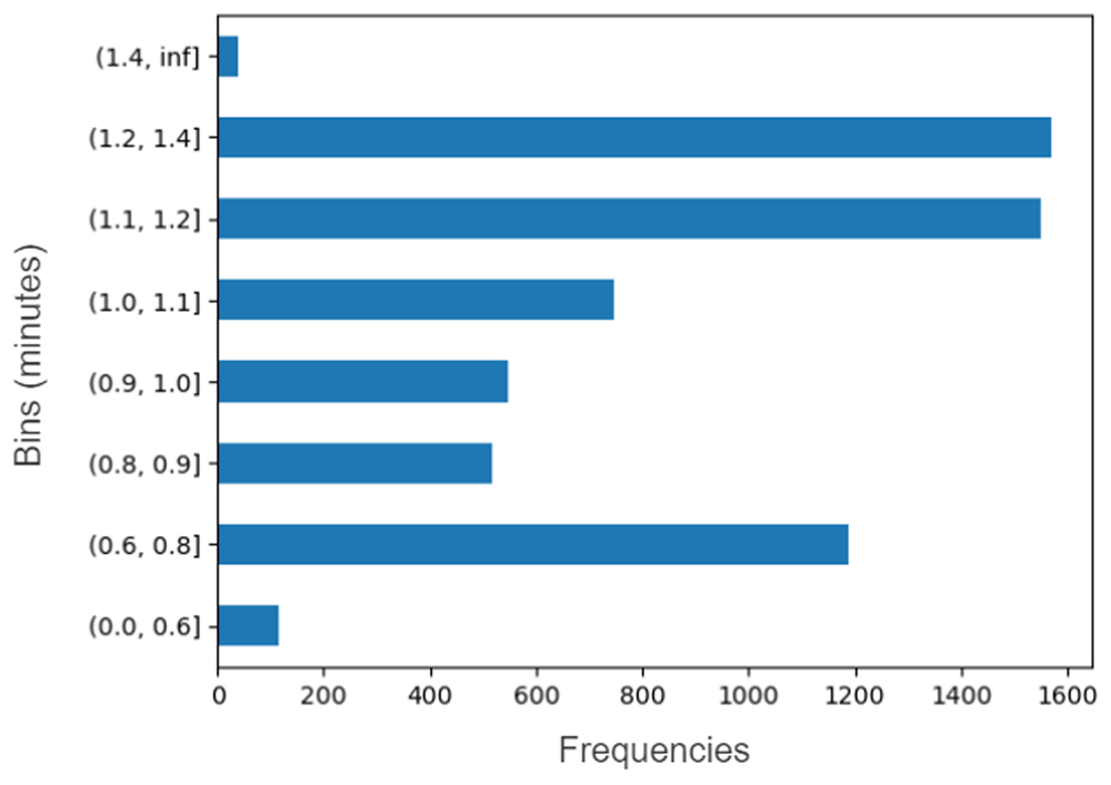
Figure 3. Cycle time span in minutes.
between 1 to 2 minutes, with relatively fewer instances exceeding these bounds in either direction. A visual inspection then could suggest that instances lying inside these cycles could potentially be flagged as anomalies, thus this serves as a first indication that cycle variance/duration could potentially influence the anomaly detection process. Expanding on that idea, using feature engineering, a new feature is formed that exploits the temporal dynamics of the detected cyclic component, which is also integrated into the original data set, as described in Section 2.2 above.
3. Methodologies for anomaly detection
As mentioned in Section 2, the field of anomaly detection revolves around two main paradigms, supervised and unsupervised methods. Novel multi-modal deep-learning based algorithms have proven rather effective, particularly on manufacturing data sets32, however, two fundamental limitations pose serious obstacles in practice. The first limitation arises from the large amounts of labeled data that are required to train these models. The second implication is closely tied to the data set, since it pertains to the high labor cost associated with this labeling process, adding to the overall complexity. In this work, both supervised and unsupervised methods are explored to solve the defective part detection task.
3.1 Unsupervised methodologies
To mitigate the issues presented previously, unsupervised models with the ability to disentangle latent data patterns can be exploited, serving as a more scalable and versatile solution. Unsupervised algorithms operate under the implicit assumption that normal instances dominate the data set, meaning that anomalies are considerably less prevalent (definition of an anomalous point).
3.1.1 Isolation Forest. Isolation Forest (IF)33 algorithm, which can be visualized as a tree structure, consists of a collection of Isolation Trees that use recursive random partitioning to isolate observations. For outliers, fewer splits are needed, whereas, for inliers, more splits are needed. It applies an unsupervised learning methodology to identify out-of-the-ordinary data points, which may then be eliminated from the training set. Whilst other outlier detection algorithms attempt to form a profile of normal instances and then identify instances that do not fit that profile, IF explicitly isolates anomalous entries by utilizing inherent anomaly properties; atypical values for the set of covariates. The scikit-learn library provides an implementation of the IF algorithm.
3.1.2 Local Outlier Factor. Local Outlier Factor7 (LOF) is an algorithm for detecting anomalous data points, which determines a given data point’s local deviation from its neighbors by computing a given data point’s local density deviation with respect to adjacent points. LOF uses the Reachability Distance (RD) as an additional measure to produce more stable results within clusters. The RD equation for X and Y points is given below:
3.1.3 Empirical cumulative distribution-based for outlier detection. Empirical Cumulative distribution-based for Outlier Detection (ECOD)34 presents a novel unsupervised technique that falls under the statistical category of methods. The leading motivation behind this work was to formulate a parameter-free method that is also scalable, by leveraging one of the fundamental properties of outliers, the fact that they appear rarely. Modeling them as empirical cumulative distributions and concentrating on their tails, enables robust and interpretable detections. It is implemented in the Python library, PyOD8.
3.1.4 Auto Encoder. Deep AutoEncoders (DAE) are commonly exploited in anomaly detection tasks35. The deep AE module is trained without supervision and then it can be used to detect anomalies in new data. An AE module consists of two parts: an encoder and a decoder. The encoder takes the input data and compresses it into a lower-dimensional representation. The decoder takes this lower-dimensional representation and reconstructs the original input data. If the reconstruction error is high, then that serves as an indication that the input data is anomalous. On the contrary, a low reconstruction error, translates to an accurate reconstruction after decoding, meaning that the network has adequately compressed all the relevant information in its latent representation. For the training of deep AE, the loss function of Mean Absolute Error (MAE) is commonly used (see the following formula).
where n is the number of data points, Yi is the actual value of the ith data point, and is the predicted value of the ith data point. Finally, the threshold was selected in a dynamic fashion based on the mean and standard deviation of the MAELoss depicted in the following formula:
where:
where n is the number of data points, xi is the actual value of the ith data point and is the mean of the whole instance.
3.1.5 Anomaly transformer. Anomaly Transformer (AT), calculates the association discrepancy using a cutting-edge Anomaly-Attention mechanism36. In six unsupervised time series anomaly detection benchmarks of three applications-service monitoring, space & earth exploration, and water treatment, the AT achieves state-of-the-art results, surpassing previous works. The basic transformer architecture (see Figure 4) is altered to cater to the time series domain, using the AT as mentioned previously. Transformers have made noteworthy advancements in numerous fields, including time series analysis, machine vision and natural language processing. Their outstanding capability in unified modeling of global representation and long-range relationships is credited with this performance.
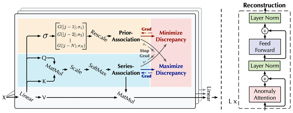
Figure 4. The proposed Anomaly Transformer architecture.
The anomaly score for an instance X is computed as follows:
where n is the number of data points, Xi is the actual value of the ith data point, is the predicted value of the ith data point and P and S refer to the learned prior and series associations respectively. Anomalous points tend to exhibit lower association discrepancy scores, however, the overall anomaly score remains largely unaffected.
3.2 Supervised methodologies
Considering the supervised machine learning methods employed in this study, greater emphasis was given to the rule-based anomaly detection methods, since they gave us the ability to use even more advanced methods, such as ensembles and progressive learning. Additionally, this way interpretability techniques that solely use the internal structure of the model can be applied, rather than using external transparent models (such as decision tree surrogates that mimic the behavior of the black-box model) to derive interpretations for the predicted results.
3.2.1 Random Forest. Random Forest (RF) is a homogeneous learner, using a combination of decision trees under an equal voting scheme37. This methodology is widely known as Bagging, or bootstrap aggregating, and trains multiple learners in a series of independent, same-sized subsets of the data. The only prerequisite that these subsets should follow, is that they should have comparable distribution to the original data, while their sampling can be done either with or without replacement. The Random Forest used in this work adheres to the methodology of Classification And Regression Trees and the implementation can be found in Python scikit-learn library. Comparative studies support the superiority of Random Forest models over decision trees in the majority of undertaken tasks38.
Since in this scenario, anomaly detection can be thought of as a binary classification problem, a binary Random Forest classifier can be trained and utilized to inform us about anomalous samples depending on their attributes39. A visual representation of how a Random Forest works, is shown in Figure 5. In binary classification, the predicted outcome is the one supported by the most learners (majority voting), thus, the quorum of the votes (half plus one votes) is needed.
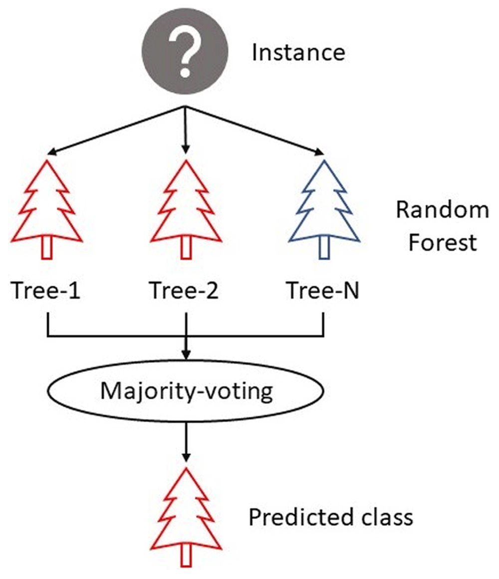
Figure 5. Process followed by Random Forest in Binary Classification.
3.2.2 Uncertainty Forest. As described in Section 3.2.1, each tree of a Random Forest consists of multiple nodes, each of which iteratively gets split into child nodes until no more splits can occur, and leaf nodes are created. Because each split is solely created based on the Gini impurity measurement, posterior class estimations from leaf nodes lean toward certainty. As an attempt to eliminate this biased behavior, Perry et al. proposed Uncertainty Forest (UF)40, based on a property called Honesty41.
The primary distinction between Random Forest and Uncertainty Forest is that the latter does not use all training samples for the development of individual estimators that the forest is comprised of. Rather, training data are separated into two subsets. Instances, along with their responses (X, y), that reside in the first subset of data, are exclusively used to generate the desired internal node splits (similar to Random Forest), whilst instances that belong to the second subset of data (held-out data), are only used to estimate the class that each node should predict. This procedure is referred to as Honesty, since it resembles the evaluation process of machine learning models. The two subsets are typically split into 67% and 33% ratios respectively.
3.2.3 Progressive Learning. Traditional machine learning models normally get trained on a specific task from scratch, without employing any prior knowledge. Transfer learning is an improvement to this, where a model can retain knowledge of previously undertaken tasks while simultaneously improving its performance on future tasks. One disadvantage of such methods is that knowledge is only transferred forwards, while their performance on previous tasks tends to degrade. This issue can be addressed with lifelong learning or progressive learning42, where the objective is to improve the model’s performance on both future and past tasks with any newly examined data (backward and forward training), by synergistically combining new models with previously trained ones.
The approach used in this study is known as Synergistic Forests (SynF), a progressive learning technique based on ensembles of decision forests. As shown in Figure 6, each learner of the ensemble is decomposed into three components namely an encoder, a channel, and a decoder.
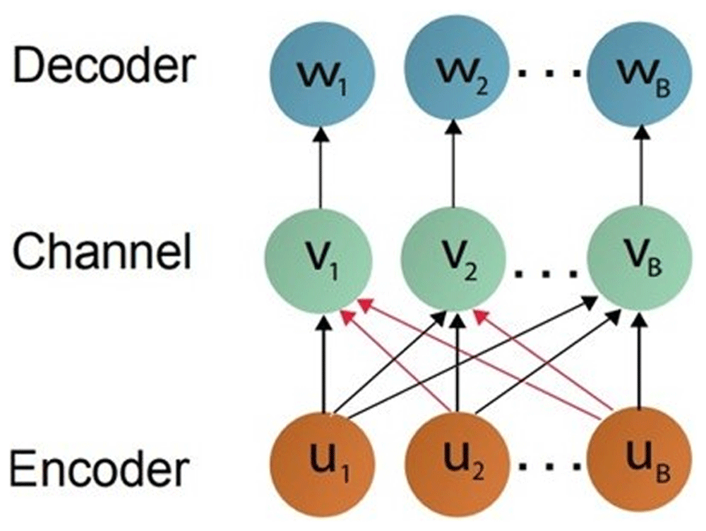
Figure 6. Architecture of Synergistic Forests.
During the encoding phase, training data are used to teach the decision forest on a specific task. Held-out data are used to generate the channels, which represent posterior probabilities of leaf nodes (probability of the examined instance being anomalous or not). As a result, each channel integrates information across all representations learned by the tree estimators, rather than their actual predictions. Finally, the decoder generates a singular prediction by applying argmax over the posteriors of all channels. The single task version of Synergistic Forest simplifies to the Uncertainty Forest approach presented in Section 3.2.2.
The general idea behind this strategy is that representations of data instances can be independently used in the ensemble. This procedure eliminates future bias, while simultaneously permitting interactions between current and past instances with the use of channel layers, achieving this way progressive learning. Extensive experimentation shows that Synergistic Forest outperforms competitors in terms of the accuracy of the predictions, along with the amount of backward and forward transfer of learning on new tasks.
3.3 Explainabillity
In addition to the anomaly detection models described in the preceding sections, two interpretability techniques are also included as an attempt to offer valuable information about how the end results provided to the user were created. Two model-specific approaches are employed, the well-known LionForest, and the proposed approach MLW-XAttentIon, used on supervised Random Forest and unsupervised transformer based learning respectively. A brief description of how both explainability methods work is given below.
3.3.1 LionForest. Ensemble models, such as Random Forest, have gathered a lot of attention over the years, due to their highly accurate predictive performance on a plethora of tasks. Despite the fact that they consist of multiple decision trees, which are considered intrinsically interpretable and are able to provide reasons for their outputs, Random Forest models are considered opaque and provide no additional information about how their final prediction was created. For this purpose, the Random Forest-specific interpretability approach Local Interpretation of Random Forests (LionForest) is included in this study, which is able to handle both classification and regression tasks43.
The objective of LionForest is to learn a Random Forest model (binary classifier in this study) on a specific task and provide the end user a singular conclusive rule with the features, ranges of features, and the corresponding prediction (normal/defective), in natural language. The term conclusive refers to the properties every generated rule should follow. More specifically, a generated rule is considered conclusive if the following statements hold true:
1. If features included in the rule are modified within the defined ranges, the final prediction will remain the same,
2. If features excluded from the rule are modified into any possible value, the prediction will remain the same.
An intuitive example of the use of conclusiveness can be presented with the help of Figure 7, where the structure of a single decision tree is visualized. For an instance with features [f1 = 2, f2 = 1, f3 = 9, f4 = 3], the conclusive rule produced by the tree would be: if F1 ≤ 4 and F2 ≤ 5 then Defective.
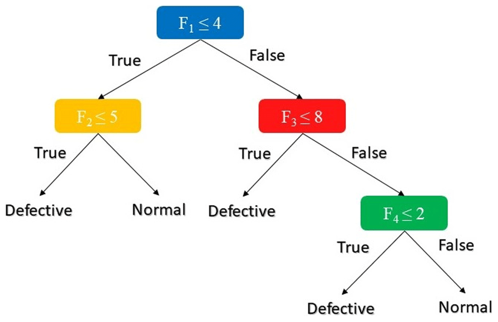
Figure 7. Internal structure of a decision tree.
LionForest works in a similar way, by combining all paths found on the Random Forest’s estimators, with the objective to provide a final rule with the least possible features, while still maintaining conclusiveness. To achieve this result, three processes should be followed, namely path reduction, feature range extraction, and rule composition.
3.3.2 MLW-XAttentIon. Multi-head attention is a module for attention mechanisms that iterates through an attention mechanism several times in parallel. The independent attention outputs are then concatenated and linearly transformed into the expected dimension. Intuitively, multiple attention heads allow for attending to different parts of the sequence (e.g. longer-term dependencies versus shorter-term dependencies). In theory, this allows for the network to discover a richer final representation of the input data.
One of the most popular methods for achieving explainability in deep learning models is through attention mechanisms44. Attention mechanisms are used to determine which parts of an input instance are the most significant contributing factors for a given output. This can assist in explaining why a model made a specific decision or prediction.
Leveraging the anomaly attention mechanism described in subsection 3.1.5 and the weights associated with each stacked attention layer a weighted-average multi-layer attention explainability method is proposed denoted hereafter as Mean-Layer-Weight-Explainable-Attention or MLW-XAttentIon. The intuition behind this approach is to utilize the overall average anomaly attention score of the encoded weights over N attention heads and M stacked anomaly layers for each of the input features. The final output is an unbounded value representing the arithmetic mean from the concatenated mini-batch evaluation steps during inference. A variant of this pipeline entails the use of the association discrepancy mechanism of the transformer, which enhances the separation of normal-abnormal points, by scaling each final feature score with that value, resulting in a less biased estimation.
The final scores are presented in a bar plot, closely resembling the Shapley format45 where the value attributed to each feature in a model’s prediction is based on how much that feature contributes to the prediction (anomaly or normal).
4. Experimental results
This section is dedicated to presenting the results gathered throughout this study and will be divided into three parts, the experimental setup procedure, the evaluation metrics used to determine the performance of the machine learning models, and the results section, where the performance of all methods is comparatively presented.
4.1 Setup
In this section, the experimental setup along with the selected parameters to train our unsupervised and supervised machine learning models is presented. This is largely an ad-hoc setup when it comes to unsupervised learners, where the parameters are carefully selected after extensive trial-and-error testing on our data set. In supervised methods however, parameter optimization (i.e. cross-validation) is feasible, and as a result, the final parameter selection was guided by a grid-search cross-validation strategy that performs an exhaustive search over specified parameter values for each estimator.
At this point, a distinction between the DL and non-DL methods is made, starting with Table 3 which contains the training parameters for the latter estimators9,10. For the parameters optimization of each model, exhaustive grid-search was used, in order to consider all parameter and go through many possible pipelines.
Table 3. Experimental setup for Isolation Forest, Local Outlier Factor and Empirical Cumulative distribution-based for Outlier Detection anomaly detection methodologies.
| Method | Parameter | Value |
|---|
| IF | Estimators | 100 |
| Max features | All |
| Bootstrap | True |
| Warm start | True |
| LOF | Neighbors | 20 |
| ECOD | Contamination | 0.1 |
Moving on to DAE, this architecture is comprised of four encoding and four decoding, non-linear, fully connected layers to compress the input signal into a lower, 10-dimensional, latent space. The threshold to label a point as anomalous is defined in equation (2). The complete architecture is depicted in Figure 8.
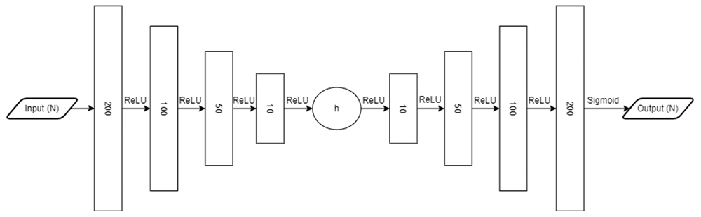
Figure 8. Deep AutoEncoder architecture for anomaly detection.
Finally, the parameters of the AT are presented in Table 4 below. It is worth noting that an early stopping criterion was imposed to halt training and save the parameters (weights and biases) of the best-performing model on a separate validation set.
Table 4. Anomaly Transformer parameters.
| Parameter | Value |
|---|
| Initial learning rate | 0.005 |
| Batch size | 32 |
| Anomaly ratio | 10 |
| Max epochs | 20 |
| Layers | 3 |
| Window size | 30 |
As mentioned previously, supervised learners can benefit from cross-validation techniques to better estimate the optimal parameter values. A typical grid search approach will attempt to fit different estimators using all the possible combinations of the parameters provided. Consequently, the total search space grows exponentially as the number of possible values increases, which in turn raises the total computational time. To mitigate this issue, only a handful of initial parameters were chosen, which, we believe, serve as a reasonable starting point for our particular data set. Also, the original data set is split, in a deterministic fashion, into three sets, training, validation and test set, with 75%–15%–15% ratios over the original data respectively. An additional parameter, “stratify’’, ensures that class frequencies are approximately preserved in each train and test split. Table 5, contains the set of initial parameters considered for the Random Forest classifier, while optimal values are marked in boldface after cross-validation based on F1 score.
Table 5. Grid search cross-validation ijitial search space for Random Forest.
| Parameter | Possible values |
|---|
| Estimators | 100, 300, 500 |
| Max depth | None, 3, 32 |
| Split criterion | ‘Gini”, ’Entropy” |
| Min samples (split) | 2, 5, 10 |
| Min samples (leaf) | 1, 5 |
| Max features | ‘sqrt”, ’log” |
Since all supervised methods that have been employed are based on tree models, similar parameters to Random Forest were utilized on both Uncertainty Forest and Synergistic Forest, with the only limitation being that Uncertainty Forest allows the user to modify only the number of estimators and the maximum depth of the tree.
4.2 Evaluation
To evaluate the predictive capabilities of the unsupervised and supervised models, four performance metrics are utilized, namely accuracy, precision, recall, and F1 score. The formulas used to calculate each of these metrics are presented below.
where:
and:
True Positive11 (TP): the classifier correctly predicted the Positive class.
True Negative12 (TN): the classifier correctly predicted the Negative class.
False Positive (FP): the classifier falsely predicted the Positive class.
False Negative (FN): the classifier falsely predicted the Negative class.
While accuracy measures the proportion of the correctly predicted instances out of all predictions, more often than not, more nuanced insights about the results are required, especially with imbalanced data or when certain types of faulty predictions can be critical. In this case, class imbalance was not evident, but, insights about the type of error the model made could be useful. Thus, recall (proportion of predicted anomalous instances that are actually anomalous), precision (proportion of actually anomalous instances that got correctly predicted), and F1 (harmonic mean of precision and recall) were taken into consideration.
4.3 Results
In this section, the experimental results are presented with reference to the performance of the machine learning models (supervised & unsupervised) and at the same time, introduce informative graphs to elaborate on the transparent artificial intelligence solution developed in Section 3.3. Table 6 presents the benchmark results for all the examined machine learning methods on our data set.
Table 6. Experimental results of machine learning models.
| Method | Accuracy | Precision | Recall | |
|---|
| Unsupervised | IF | 0.4872 | 0.4673 | 0.1228 | 0.1945 |
| LOF | 0.4949 | 0.4887 | 0.0399 | 0.0738 |
| ECOD | 0.4940 | 0.4905 | 0.0952 | 0.1594 |
| AE | 0.4968 | 0.5031 | 0.1479 | 0.2287 |
| AT | 0.8967 | 0.8628 | 0.9158 | 0.8885 |
| Supervised | RF | 0.9013 | 0.8994 | 0.9055 | 0.9024 |
| UF | 0.8923 | 0.8889 | 0.8987 | 0.8938 |
| SynF | 0.8994 | 0.9000 | 0.9006 | 0.9003 |
Focusing first on the unsupervised methods, the superiority of the AT over the rest of the methods is evident across all the studied metrics. More specifically, a ≈78.6% increase in accuracy is observed compared to the baseline methods. The AT also excels in the weighted F1 score on account of its high precision and recall relative to the other four methods. The fact that most unsupervised models failed to correctly identify the basic makeup of the abnormal instances may be related to the data’s high dimensionality and complexity. As a result, their forecasts may be compared to a random selection process. An interesting observation surrounding the AT’s recall, being much greater than the rest (even supervised) suggests that it proved quite accurate at anticipating anomalies. It would appear then, that harnessing the power of attention-based methods leads to a note-worthy improvement in prediction accuracy when it comes to high-frequency sensor data.
Regarding the supervised machine learning methods, a similar performance is observed across all three techniques, with Random Forest having a slightly better performance than Synergistic Forest. It is important to mention that Synergistic Forest was introduced as a progressive learner, with the ability to perform both forward and backward learning while getting trained on new data. For this purpose, we attempted to test this aspect of learning ability on Synergistic Forest, compared to Random Forest. Specifically, the original training data is split into 10 equally sized subsets. Both methods were trained on each subset sequentially, with the addition of 1 estimator whenever a new subset was queued for training, for a total of 10 after the models were trained on all subsets. Table 7 presents the performance of the models on the first subset of training data, once before and once after all subsets were queued for training.
Table 7. Progressive learning of Synergistic Forest compared to Random Forest, before and after complete training.
| Before | After |
|---|
| RF | SynF | RF | SynF |
|---|
| Accuracy | 0.8369 | 0.7843 | 0.9773 | 0.9856 |
| Precision | 0.8545 | 0.8261 | 0.9899 | 0.9806 |
| Recall | 0.8310 | 0.7466 | 0.9666 | 0.9921 |
| 0.8426 | 0.7843 | 0.9781 | 0.9863 |
It is clear that, even though Random Forest was able to get better performance on the training phase of the first subset of data, Synergistic Forest was able to boost its predictive ability on previous sets of data whenever a new training phase was initialized.
Interpretability of Random Forest was achieved with the use of LionForest, where explanatory rules are created for individual instances. Figure 9 shows the five most important features along with their ranges, demonstrating that instances consisting of those features that lie in between those specific ranges are considered anomalous.
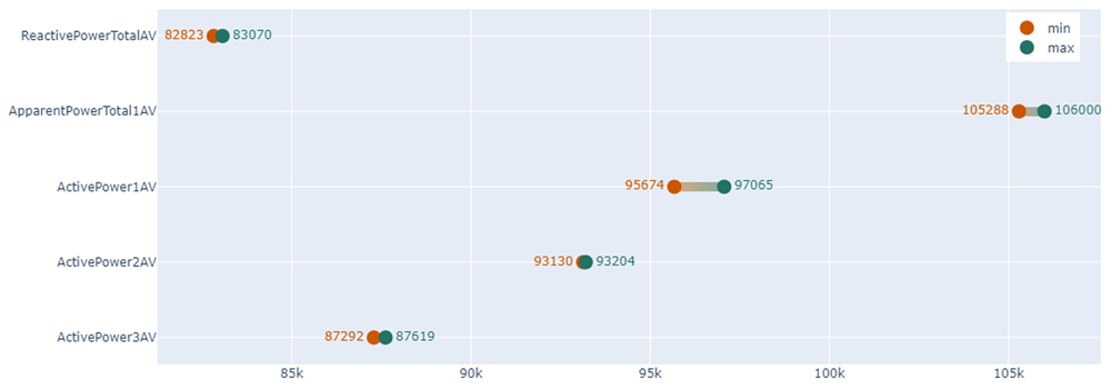
Figure 9. Ranges of the most important features of an anomalous instance.
To get a better understanding of the helpful impact that interpretability adds to anomaly detection, a specific example further analyzing Figure 9 will be provided as follows. Since the examined instance is considered defective, by applying all these conditions on the data the model was trained on, it is expected that all instances that follow these conditions should be defective as well. Specifically, the total amount of data following the condition ActivePower1AV ≥ 95674 & ActivePower1AV ≤ 97065 are 880, 437, of which are labeled as defective (≈49.6% defective). By further adding one more condition (ActivePower2AV ≥ 93130 & ActivePower2AV ≤ 93204) there are 2 total samples present, both considered defective (100% defective), proving the aforementioned assumption. The more conditions added, the more accurate the result, but the likelihood of new samples following all the conditions decreases, thus, the amount of conditions needed varies based on the underlying application.
The following plot illustrates the intuitive manner in which the second XAI method, MLW-XAttentIon, demystifies the AT inference mechanism. A feature’s contribution to the average data set predictions vs the prediction of a particular instance is represented by its value. The height of each bar represents the magnitude of the contribution for that feature. Positive (negative) values indicate that the feature causes a positive (negative) impact on the prediction. Based on Figure 10, which represents an average over all the samples at inference time, feature ActivePower1AV has the strongest positive impact whereas ActivePower2AV most negatively contributes to the predictions.
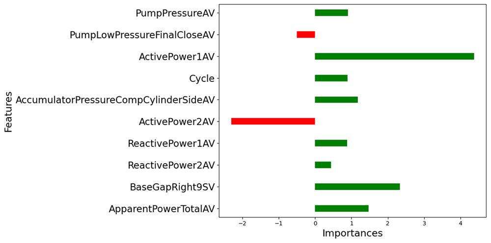
Figure 10. MLW-XAttentIon feature importance scales on experimental data set.
5. Conclusions and summary
In this work, the ability of a total of seven supervised and unsupervised machine learning methods is compared in order to tackle the significant problem of identifying abnormal behaviors in day-to-day operations of an automotive industry. The Anomaly Transformer showed significantly better results compared to the rest of the unsupervised methods, with an accuracy of ≈89.7%, slightly outperforming even a supervised method in this metric. An intriguing discovery is that the recall of the Anomaly Transformer was significantly higher than precision (≈ 6.1% higher), implying that the model is better at identifying truly defective parts (true positives) out of all the defective instances in the dataset rather than it is at avoiding misclassification of defective instances (false positives).
Regarding the supervised models, Random Forest marginally outperforms Uncertainty Forest and Synergistic Forest across all metrics. The use of labeled data seems to have resulted in the creation of more robust models. Further testing between Random and Synergistic Forest showcases that the over-time learning ability of Synergistic Forest on batches of data proved to be superior to the learning ability of Random Forest. This comes as a result of the introduction of both forwards and backwards learning on the former method, in which an accuracy increase of ≈25.6% was observed compared to ≈16.7% for the random forest when the models were tasked to handle batches of data and retrain themselves.
Looking into the experimental results during the evaluation process, we are able to answer the question "Are unsupervised anomaly detection models comparable to supervised models in the industrial field?". A very important insight that was uncovered in this work, is the accentuation of the potential of novel unsupervised approaches compared to supervised methods in Industry 4.0 applications. Domain specific labeled data are frequently difficult to obtain, while trying to label existing data is equally hard, due to the frequently generated data by sensors. In this work, we evidently provide results showcasing the comparable predictive performance that state-of-the-art unsupervised models can achieve over supervised models, overcoming the necessity for labeled data when they are not available. It is important to mention that standard unsupervised models (e.g. IF, LOF) were unable to provide comparable results, probably attributed to the high complexity of the data, which was successfully handled only by the Anomaly Transformer. On the other hand, all supervised models behaved similarly, indicating that the presence of labeled data can lead to more robust models.
Finally, interpretability methods were utilized as an attempt to provide reasons for the outputs of the two best-performing techniques (MLW-XAttentIon for Anomaly Transformer and LionForest for Random Forest). Both methods were able to highlight similar features that influenced the final decision the most, with the only difference being that LionForest was also able to provide the ranges of the respective features, which in turn means that, given adequate monitoring intervals, early detection of defective parts is definitely within reach under real-time circumstances. Adopting XAI methodologies uncovers insights into the models’ behavior, increasing trust between humans and AI, leading this way to ethical, trustworthy and bias free predictive models.
The answer to the second question "Does explainable AI offer an added impact in anomaly detection problems?" is given below. By presenting feature importances, process specialists may discover any flaw in the predictive performance via a visual examination, especially when misclassifications occur more frequently than usual. Features that influence these instances the most, can be further inspected and the possibility of concept drift can be considered, where some aspects of the manufacturing process have been altered but were not taken into consideration up until that point. If this is the case, updating the models with the appropriate data would solve the issue. On the other hand, if no change was performed regarding the manufacturing process, an inspection of the sensors providing the respective data for those features should be undertaken, to eliminate the possibility of any malfunction on the sensor measurements.
Moreover, a future research direction would be to explore ways to integrate other model-agnostic explainability techniques, like SHAP or LIME, into anomaly detection models, aiming to provide more transparent insights into how these models arrive at their decisions. This approach revolves around bridging the gap between the high predictive performance of anomaly detection models and the need for interpretability in anomaly detection systems, making them more accessible and trustworthy for end-users and domain experts.
Ethics and consent
Ethical approval and consent were not required.