Introduction
The European Union has adopted the goal of reducing greenhouse gas emissions by at least 55% by 2030 and to become climate neutral by 20501. To achieve this in the transportation sector, the automobile industry has been shifting from internal combustion engines to electric vehicles (EVs). Despite the reduction in carbon footprint, this transition brings about new challenges, particularly in terms of electricity demand and grid management. As most EV charging events occur at home, uncontrolled charging of EVs in greater numbers might put pressure on the power grid2.
To avoid the peak electricity demand, EV charging flexibility is introduced to shift electricity demand to a preferred time, instead of charging the EV instantly when it is plugged in. The flexible charging strategy adjusts the charging time and rate in regard to the grid demand, electricity tariffs and the availability of renewable energy generation3. Flexible charging of EVs can reduce charging costs by 30% and grid operational costs by 10%4. Based on a case study of a predicted 5 million EVs in California in 20255, managed charging strategy was predicted to reduce renewable curtailment by up to 40% compared to uncontrolled charging strategy.
More recently, bidirectional charging strategies which allow the EV to discharge back to the power grid or the household have gained interest. This gives rise to the concepts of Vehicle to X (V2X) with vehicle-to-grid (V2G) and vehicle-to-home (V2H) strategies6 being among the most common. Compared to V2H, V2G requires more sophisticated grid infrastructure, regulations and complex control strategies to discharge the power from multiple aggregated EVs to the grid7. By comparison, V2H can work “behind the meter” as an alternative controllable load/generator to offer home energy savings for EV users on a small scale, and providing a backup power supply in the case of grid outage. To effectively implement the V2H strategy, a home energy management system (HEMS) is required to monitor and control energy generation, storage, and consumption within a household, thus optimizing the self-sufficiency and cost reduction8.
A heuristic method for V2H has been presented in 9 to find the optimal charging and discharging hours for an EV battery to flatten the load demand and minimize the electricity bills in a day-long period from a real-time application. Smart homes combined with small-scale distributed photovoltaic (PV) and EV can decrease daily electricity costs10, and the study in 8 found that V2H implementation with PV could reduce daily electricity costs by 20%. Compared to the HEMS with PV and a stationary battery, the integration of an EV and PV is better from an economic perspective, because the EV battery has dual functionality for both transportation and energy storage11. Also, the EV battery usually has greater capacity than a stationary battery, which better maximizes the self-consumption of PV and offsets more household demand into off-peak times.
A case study based on a smart German household investigated the effects on V2H cost savings by varying EV battery capacity, household electricity demand, PV generation, EV charging rate, PV export tariff, and driver profiles12. V2H applications in Netherlands13, UK14, and Japan15 have also been investigated. It was found that the combination of PV generation with a stationary battery or V2H save up to 30% on electricity bills regardless of the electricity tariff and a 3-tier tariff can further bring about a reduction of up to 85% in the electricity bills with the Nissan Leaf 2018 EV14. Additionally, a V2H system has been found to improve the PV self-sufficiency rate in households whose annual PV generation exceeds their annual electricity demand15. According to the aforementioned studies, V2H cost savings are highly influenced by electricity tariffs, household demand, and PV generation. This paper aims at developing V2H models based on a non-commuting EV profile and a commuting EV profile. Results are presented for a case study using data related to Irish households. The model allows us to the study of the potential for V2H to minimize annual electricity costs and to study the impact of parameters such as PV capacity, household demand, electricity tariffs and vehicle usage on the savings. This work also quantifies the economic benefits to an EV owner by investigating the net present value (NPV) and the discounted payback period (DPP) across a range of investment costs and discount rates. The contributions of this work include the extension of quantification of cost savings due to V2H to a variable electricity tariff structure, specifically a commonly used 3 tier (Day/Nigh/Peak) tariff. The work also includes a more comprehensive sensitivity analysis by including the sensitivity of V2H savings to additional variables such as day and night tariff disparity, EV usage and allowable EV battery depth of discharge (DoD). It is found that V2H savings are largely influenced by EV usage and are most significantly affected by the difference between the day and night tariff with a +20% and -50% variations in electricity tariff difference resulting in ±60% changes in V2H savings. It is also found that, under the 3 tier tariff structure the costs savings from implementation of V2H slightly decline with an increase in installed PV capacity which is in contrast to the findings in 12 which were conducted for a flat tariff structure.
This paper is organised as follows: The Method Section describes the model configuration, data acquisition, V2H model constraints, flexible and uncontrolled charging methods and net present value methodology. Results are presented and analysed in the Results and Discussions Section with the main conclusions from the study presented in a final section.
Method
Overview of modelling approach
The methodology is based on the use of an optimization model which minimizes home energy costs over the course of one year. The model takes as input hourly profiles for home electrical energy assuming use of a heat pump for heating, generation from PV, an EV usage profile, and tariffs for import and export of electricity from/to the grid. The primary objective is to optimize the charging strategy of the EV and use of PV generation in order to optimize home energy usage so as to minimize energy costs for the home owner. Uncontrolled, flexible uni-directional charging and full flexible bi-directional (i.e. V2H) charging strategies are considered. Energy costs for a baseline model are first considered and a sensitivity analysis is performed to understand the sensitivity of the cost savings to variations in various assumed baseline parameters relating to the household and the EV. The results of the optimization are used to assess the business case for a home owner using a net present value analysis. The optimization model is implemented using the Spine modelling platform and makes use of the SpineOpt tool for the optimization16. The Spine modelling toolbox17 and SpineOpt18 are freely available to use under the GNU Lesser General Public License v3.0. Spine is a flexible open-source energy system modelling framework developed in Julia16. The EV driving data, household demand data, PV generation data and water and space heating data (for the heat pump) are critical inputs for the optimization model to determine the EV battery state-of-charge (SOC), charging and discharging power, electric power imported from grid, etc. These inputs are described further in the section below.
Model configuration
A model in Spine is represented as a set of nodes, units and connections. In general nodes are points where energy flows are balanced and may also incorporate energy storage. Units represent energy conversions, e.g. a generator which converts the fuel to electricity. Connections represent energy flow between nodes, the physics for which can be defined in general to represent any kind of flow (electricity, gas, etc.). For the V2H model the nodes, units and connections are shown in Figure 1. This configuration is set up to represent the possible energy flows between the household, PV generation, space and water heating electrical demand, EV charging, and the grid. The model aims to optimize the energy flows, so as to minimize energy costs based on time-varying electricity tariffs with a set of predefined inputs and parameters.
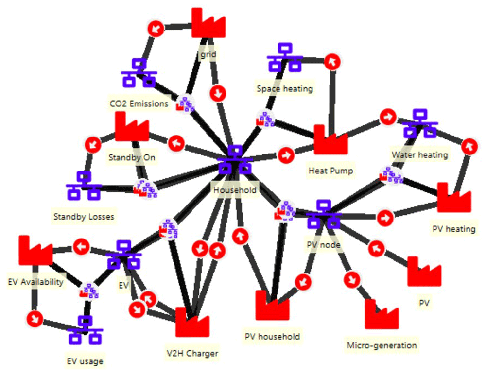
Figure 1. Configuration of V2H model.
The functions of each node and each unit are described in more detail in the following:
Household: The Household node has an associated hourly household electricity demand throughout the year. This node facilitates all the flows in the model, as the electricity from the grid (Unit) or EV (Node) must pass through the Household node to reach the Heat Pump unit, the EV node, and the Standby Losses node.
PV system: The PV unit determines the hourly on-site PV generation. The PV node obtains the electricity from the PV unit to distribute this electrical power to the other units or nodes. After being consumed by the household and water heating demands, the excess PV generation is supplied to a Micro-generation unit. The PV household and PV heating units facilitate the flow of electricity from PV node to Household node and to Water heating node respectively. This micro-generation unit essentially represents electricity exported to the grid from the PV system which receives a payment according to a predefined hourly export tariff.
HP system: The Heat Pump unit consumes energy from the household node to meet space and water heating demands, which are denoted by the Space heating and Water heating nodes, respectively.
EV system: The EV node stores energy, and has an associated battery state of charge (SOC). The V2H Charger unit defines the hourly plug-in status of the EV charger and facilitates the EV charging and discharging between the EV node and the Household node. The charger capacity and efficiency are defined in the connections between V2H Charger unit, Household and EV nodes. The EV Availability unit defines the EV (essentially whether the EV is at home or away) and also facilitates the depletion of the EV battery from driving. The EV usage node defines the hourly depletion during the time the EV is away.
Standby losses: A non-constant efficiency for the V2H charger is modelled by means of standby losses and a constant efficiency. The Standby On unit determines whether EV is connected to the charger or not. The Standby Losses node determines the hourly standby losses from the EV charger at a fixed rate.
Grid: The grid unit has associated the hourly electricity prices and imported electrical power to the Household node whenever the household demand is not met by either the EV or PV nodes. The CO2 emissions node defines the hourly CO2 intensity of the grid, thus yielding the hourly carbon footprint within the household.
V2H model constraints
The primary goal of the V2H model is to minimize the annual household electricity costs under a set of parameters and constraints with the objective function defined as followed:
where pelec(t) corresponds the grid electricity prices, pexport is the constant export feed-in tariff, Pgrid(t) and Pexport(t) represent the electrical power imported from the grid and exported from the PV over all time steps t, respectively. Note vehicle to grid, i.e. export of energy from the EV battery to the grid is not allowed in this model. Hence, the V2H revenue is determined by the grid electricity imports and export from PV.
The fixed inputs include household electricity demand, HP demand, EV driving depletion, and charger standby losses, which are all supplied by PV generations, EV discharging power, or grid imports. To have the load balance, the total energy supply should be equal to the total energy consumption at a given timestamp t by:
where Pgrid(t) is the grid electricity demand, PPV(t) is the on-site PV generated power, Phousehold(t) is the household electricity demand, Pheatpump(t) is the heat-pump electricity demand, Pexport(t) is the exported power from PV, Pstandby(t) is the V2H charger standby losses, PEV,discharge(t) and PEV,charge(t) represent the amount of energy discharged from EV and charged to EV, respectively.
The standby losses Pstandby(t) is represented for V2H converter at a constant loss Pstandby,const, when the EV is connected to a charging point (bV2H_avail = 1) under the condition of neither charging (bcharge = 0) nor discharging (bdischarge = 0):
Owing to the efficiency η, the electric power discharged from the EV and charged to the EV have been curtailed by:
where Edischarge(t) and Echarge(t) represent the amount of energy discharging from the EV and the amount of energy charging to the EV battery at timestamp t, respectively, and both of them range between 0 to 7.2 kWh average for any hour.
EV depletion from driving is assumed to be a set rate per hour when it is away from home, and is represented by the energy usage from driving EEV,usage(t). The energy storage in EV battery EEV(t) at timestamp t is dependent on the energy storage at the previous timestamp t – 1, EEV(t – 1), charging power, discharging power, standby losses and EV energy according to:
In this work, the SOC is constrained to operate within a given range which is set to a minimum of 30% and a maximum of 80%. A further constraint is implemented whereby, at a certain daily departure time, tdep, the state of charge of the battery must at least have reached a minimum level SOCdep. For the baseline model the SOC must have reached at least 70% at 7am. Thus, a binary component bdep(t) is set to be 1 when it is 7am (tdep) every day, whilst bdep(t) is set to be 0 for the other hours. Hence, the constraints related to EV battery SOC are written as follows.
where EEV,max represents the rated EV battery capacity and SOCdep is given as 70%.
Flexible uni-directional and uncontrolledUncontrolled charging methods
Except for disallowing the EV to discharge, the flexible uni-directional charging model shares the same input data as the V2H model. The flexible charging model has a SOC range between 30% and 80%, and standby losses are also taken into consideration. Also, for the flexible charging mode, the minimum SOC must reach 70% at 7am every day.
The discharging process is also excluded in the uncontrolled charging mode. As long as the EV is plugged in, the charging process will continue until its SOC reaches 100%. The uncontrolled charging power PEV,charge,uncontrolled (t) is given by:
Herein, the EV charger always operates at the full capacity (7.2kWh).
Both the micro-generation power Pmicro,uncontrolled(t) and the grid electricity demand Pgrid,uncontrolled(t) in uncontrolled mode are determined by the PV generation, household demand, HP demand and uncontrolled charging power as follows:
Net present values and discounted payback period
To evaluate the business case for V2H application in a household, it is necessary to calculate the net present value (NPV) of a V2H investment across multiple years and determine its discounted payback period (DPP) under a variety of scenarios. NPV is defined as the difference between the present value of cash inflows and the present value of cash outflows over a period of time19. NPV estimates the future cash flows in comparison to the initial capital investment by:
where CFn is the net cash flow at year n and i is the discount rate and N is the number of years over which the investment is evaluated. The NPV in this work is evaluated over a period of 10 years. The cost of battery degradation20 is also taken into consideration for the net cash flows generated for a given year and different discount rates ranging from 3% to 9% are considered. The V2H investment cost Cinvest takes V2H bidirectional charger cost CV2H, installation cost Cinstall, HEMS cost CHEMS, uncontrolled charger cost Cuncontrolled, and the grant G into account by:
The cost ranges used in this study for those components can be seen in Table 1. The grant allows to take into account a grant incentive often provided by authorities to incentivise the take up of EVs. Currently the grant offered to Irish EV users is €60021. For the HEMS, costs range between €91 and €560, but the cost can further reduce to €28 with the replacement of a cheaper commercial HEMS controller22. V2H chargers are not yet widely commercially available so the cost is somewhat uncertain. For this study is assumed that the cost for V2H bidirectional charger ranges from €1500 to €7500, and the cost for uncontrolled charger is lower than €150023.
Table 1. Ranges of investment costs.
| Components | Cost range |
|---|
| Bidirectional charger | €1500 – €7500 |
| Grant | €600 |
| HEMS | €28 – €560 |
| Installation | €500 – €3000 |
| Uncontrolled charger | €1500 |
The DPP determines whether the investment is worthwhile and is calculated from:
where Y is the year before the occurrence of discounted payback period, |A| is the cumulative cash flow year in the year before payback and B is the discounted cash flow in the year after payback. A V2H system is deemed to be a worthwhile investment if the DPP is within 10 years.
Case study data acquisition
The case study is based on the adoption of V2H by an Irish household. The model inputs include household electricity demand, HP electricity demand, PV generation profiles, and EV driving profiles for the V2H application in an Irish household. The baseline household electricity demand adopts the electricity demand in an average Irish household12, which has an annual electrical consumption of 4200 kWh. Hourly HP demand data profiles are obtained from a study on 38 German households24 scaled to the average HP electrical demand for Ireland which is 3300kWh25.
Irish PV generation data from 2019 is taken from Renewables Ninja26. The baseline model assumes a PV rated capacity of 3kW with a yearly generation of 3129kWh. In this work, the baseline EV battery capacity of 57.5kWh is adopted (based on a Tesla Model Y27). The EV charging and discharging capacity Ecap is set at 7.2kWh with an efficiency of 90%. The EV charger standby losses are given at a constant of 0.05kW. In this work, EV SOC is allowed to range between 30% and 80% for V2H services, whilst at the departure hour (7am everyday), the minimum SOC must be beyond 70%.
In this work, an EV non-commuter and commuter profile are selected for comparison in the case studies. The non-commuter profile is chosen from realistic driving profiles based on German national driving data12. For the commuter profile, Irish National Transport statistics are utilised with the average daily driving distance of 33.6 kilometres28, by consuming an average energy usage of 0.2kWh per kilometre27. The electricity tariffs used for the baseline model are reflective of a typical static day/night/peak tariff from an Irish energy supplier. The electricity export tariff of 20c/kWh is also typical of a tariff available in Ireland. To summarise, the input parameters used in this work are given in Table 2, which will be applied to simulate the non-commuter and the commuter profiles.
Table 2. Input parameters of V2H model.
| Household |
| Household electricity demand p.a. | 4200kWh (Non-commuter)/
1520kWh (Commuter) |
| Heat pump demand p.a. | 3620kWh (Non-commuter)/
2485kWh (Commuter) |
| Grid electricity prices |
| Day rate (08:00 –17:00, 19:00 – 00:00) | 44.51c/kWh (off peak) |
| Night rate (00:00 – 08:00) | 23.39c/kWh |
| Peak rate (17:00 – 19:00) | 47.46c/kWh |
| PV system |
| PV capacity | 3kW |
| Electricity export price, (pexport) | 20c/kWh |
| EV system |
| Max EV charging/discharging rate (Ecap) | 7.2kW (90% efficiency) |
| EV charger standby losses (Pstandby,const) | 0.05kW |
| EV battery capacity | 57.5kWh |
| Travelling distance per day | 33.6km (Commuter) |
| EV usage per km | 0.2kWh (Commuter) |
| Max SOC | 46kWh (80%) |
| Min SOC (08:00 - 07:00) | 17.25kWh (30%) |
| Min SOC (07:00 - 08:00) | 40.25kWh (70%) |
Results and discussion
Comparative analysis of uncontrolled, flexible and V2H strategies
To provide a snapshot comparison of the impact of different charging strategies on a household Table 3 shows a breakdown of energy generation and consumption and electricity costs for uncontrolled, and optimal flexible and V2H charging strategies. For uncontrolled charging, the EV is assumed to be charged to 100% as long as it is plugged in. For flexible and V2H charging, their SOC ranges are given in Table 2.
Table 3a. Results under uncontrolled, flexible and V2H charging scenarios (non-commuter).
| Output parameter | Uncontrolled | Flexible | V2H | Units |
|---|
| Household demand | 4179 | 4179 | 4179 | kWh |
| HP demand | 3620 | 3620 | 3620 | kWh |
| Standby losses | 0 | 381 | 381 | kWh |
| EV depletion | 2529 | 2529 | 2529 | kWh |
| EV charging | 2529 | 2529 | 6240 | kWh |
| EV discharging | 0 | 0 | 3801 | kWh |
| Annual throughput | 5058 | 5058 | 12570 | kWh |
| PV self-consumption | 1533 (48%) | 2427 (76%) | 2842 (89%) | kWh |
| PV export | 1646 | 769 | 357 | kWh |
| Grid electricity import | 8782 | 8576 | 8911 | kWh |
| Electricity costs | 3174 | 2818 | 2235 | € |
Table 3b. Results under uncontrolled, flexible and V2H charging scenarios (Commuter).
| Output parameter | Uncontrolled | Flexible | V2H | Units |
|---|
| Household demand | 2050 | 2050 | 2050 | kWh |
| HP demand | 2729 | 2729 | 2729 | kWh |
| Standby losses | 0 | 304.9 | 304.9 | kWh |
| EV depletion | 2214 | 2214 | 2214 | kWh |
| EV charging | 2236 | 2212 | 3199 | kWh |
| EV discharging | 0 | 0 | 1000 | kWh |
| Annual throughput | 4450 | 4426 | 6413 | kWh |
| PV self-consumption | 946 (27.51%) | 1356 (39.44%) | 1388 (40.37%) | kWh |
| PV export | 2492 | 2082 | 2050 | kWh |
| Grid electricity import | 6344 | 6320 | 6484 | kWh |
| Electricity costs | 2042 | 1629 | 1478 | € |
The results for the uncontrolled scenario can be considered as a reference for comparison of the two optimized charging strategies. In the case of the flexible charging the optimization primarily shifts EV charging to make better use of the PV generation where possible during the day and the lower night time electricity tariffs. In the case of V2H the main additional impact of the optimization is to use the EV battery to cover household energy demand during peak time electricity tariffs. Consequently, for the optimized scenarios for anon-commuter EV profile, PV self-consumption is increased significantly from 48% in the Uncontrolled scenario to 78% in the Flexible scenario, and 89% in the V2H scenario, while for the commuter profile, PV self-consumption shows less improvement, increasing from 27.51% in the Uncontrolled scenario to 39.44% in the Flexible scenario, and 40.37% in the V2H scenario. Thus the export of PV generation is greatly reduced under the flexible and V2H charging strategies. Compared to flexible charging V2H can make further use of the household PV generation but only if the EV is at home during daylight hours.
The total quantity of EV charging is greatly increased in the case of V2H by about 2.5 times (for non-commuting users) and 1.5 times (for commuting users) compared to that of uncontrolled and flexible strategies, resulting in its PV export being much lower than its flexible and uncontrolled counterparts. The annual throughput refers to the amount of energy that passes through the EV battery in a given year, consisting of EV charging, EV discharging and EV depletion from driving. It is notable that annual throughputs under V2H are over two times (for non-commuting users) and over 1.5 times (for commuting users) higher than annual throughput under uncontrolled and flexible scenarios.
The comparison of EV battery SOC across the full year for both non-commuter and commuter profiles are illustrated in Figure 2. For uncontrolled and flexible cases, the EV battery energy usage only results from driving, whilst the energy usage of V2H is results from both driving and discharging to supply the household. Flexible and V2H strategies share the same SOC constraints from Table 2, however the time variations of the SOC under V2H are more frequent and most dense, due to the discharging to supply household electricity consumption. By comparison to the non-commuter profile, the commuter profile has more frequent variations in EV SOC, due to its higher EV depletion from Table 3.
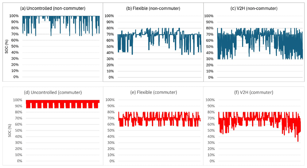
Figure 2.
EV SOC for every hour throughout the year under (a) uncontrolled (non-commuter), (b) flexible (non-commuter), and (c) V2H charging strategy (non-commuter), (d) uncontrolled (commuter), (e) flexible (commuter), and (f) V2H charging strategy (commuter).
Despite the greatly increased charging energy for V2H in Table 3, V2H presents only a marginal increase by merely 1.7% (for non-commuting users) and 9.2% (for commuting users) in the total grid electricity demand, compared to the uncontrolled charging. Also, by comparison to uncontrolled charging, flexible and V2H charging strategies lead to substantial reductions in electricity costs with a 11% reduction in energy costs (€356) using flexible charging and a 30% reduction (€939) using V2H in energy costs for non-commuting users. For a user with a commuting profile, there are a 20.22% reduction (€413) using flexible charging and a 27.54% reduction (€564) using V2H in energy costs. The average grid demand (averaged across all days of the year) at each hour of the day under the three different charging strategies is shown in Figure 3. Due to the increased PV self-consumption rates, flexible and V2H charging show significant reductions in grid demands during the afternoon and evenings, enabled by the shifting of EV charging to the night time making use of the low electricity tariffs. The V2H charging strategy further reduces peak time electricity demand bringing about significant further cost savings and reducing the grid stress during peak hours. For the non-commuting profile in Figure 3(a), the negative grid demand from 10:00 to 12:00 results from the PV export for which uncontrolled charging has the highest negative quantity. Furthermore, compared to the non-commuting profile, the commuting profile in Figure 3(b) brings about higher peaks during the night time under the flexible and V2H scenarios, and leads to deeper negative grid demand from 09:00 to 15:00 under all charging scenarios. The uncontrolled scenario for EV commuter brings about a spike during the peak hour of electricity tariff. These example results highlight the potential for V2H to significantly alter the shape of the residential energy demand profile which can clearly be used for the benefit of the home owner in terms of energy bill savings but also for the power grid in terms of reduction of demand during peak times.
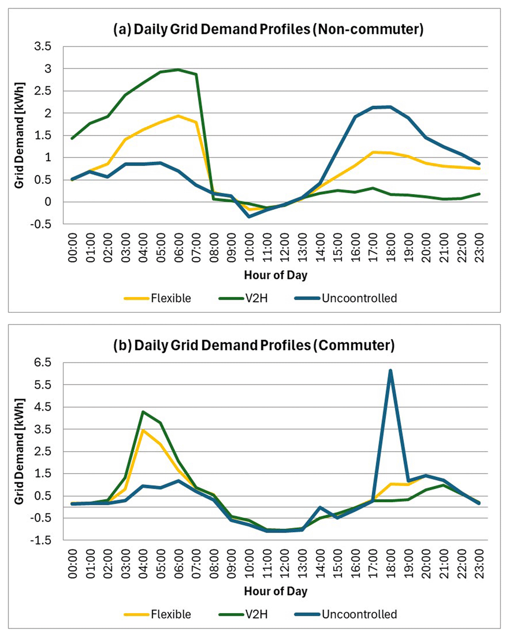
Figure 3.
Averaged grid demand for each hour of the day averaged over all days of the year (a) Non-commuter, (b) Commuter.
Sensitive analysis for V2H savings
Figure 4 investigates the dependence of the electricity costs using V2H electricity on the installed PV capacity. The dark bars show the cost savings associated with the use of V2H compared to uncontrolled charging for the same installed PV capacity. With the increase of PV capacity, total electricity costs show significant declines. Although the cost savings for V2H compared to uncontrolled charging remain high, there is actually a slight decrease with increased installed PV capacity. When using V2H, a house with no PV has a 25% reduction in total electricity costs of 1050 €/a while a house with a 6-kW PV system has a 37% cost reduction of 913 €/a on the basis of using uncontrolled charging strategy. A large portion of cost saving can be attributed to increasing the self-consumption of the installed PV system.
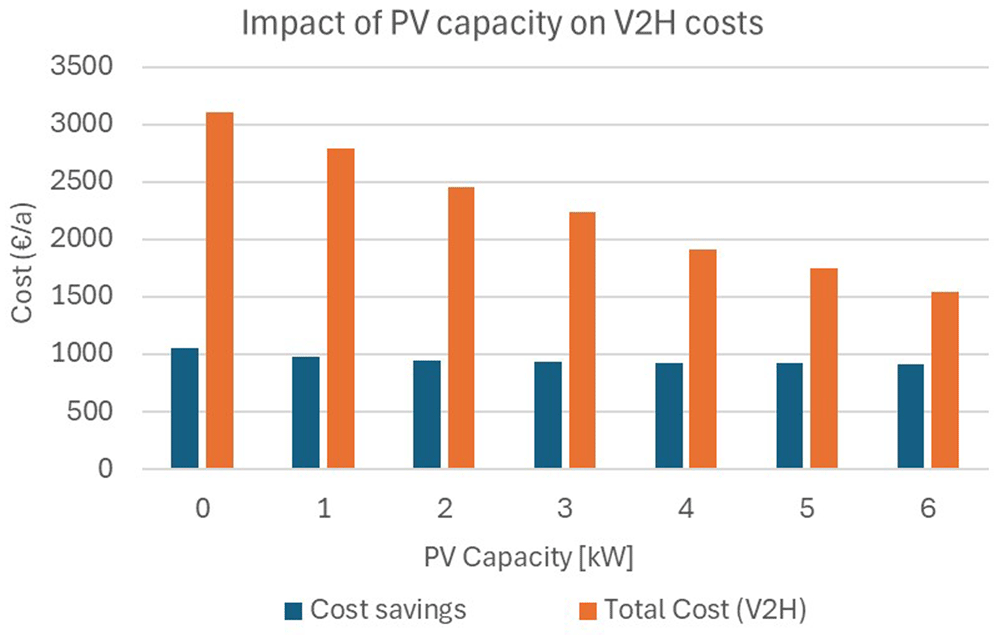
Figure 4. Impact of PV capacity on annual V2H costs.
In practice for any given household, the V2H cost savings will be influenced by the parameters such as household demand, PV capacity, day and night tariff disparity and PV export prices or EV parameters such as depth of discharge (DoD), battery capacity, charging rate, EV usage and EV availability. A sensitivity analysis is carried out to determine the key factors, which have the more important influence on V2H cost savings. The findings can be seen in Figure 5, in which the origin (0%, 0%) represents the base case parameter and savings using the parameters from the non-commuter profile defined in Table 1. The individual curves in the graphs therefore represent the change in savings relative to the base case, which results from a percentage change in the given parameter. For example, in Figure 5(a) for the curve representing the sensitivity to PV capacity, the base used a PV capacity of 3 kW with savings of approximately €2235, as shown in Figure 4. The sensitivity curve then shows the % change in savings if the PV capacity is varied from zero to 6 kW where the values are consistent with those shown in Figure 4 and show that increased PV capacity has a slight negative impact on V2H savings. The graph also shows that an increase in the PV export tariff negatively impacts V2H savings as this tends to make export of PV to the grid more favourable than using it to charge the EV.
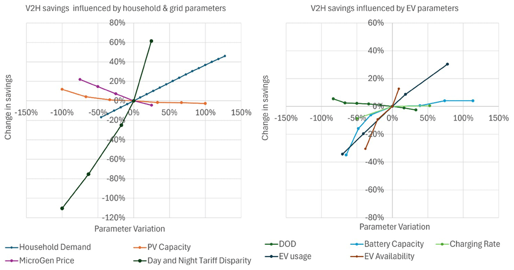
Figure 5.
Impact of various parameters on V2H savings (a) household and grid parameter, (b) EV parameters (DOD refers to EV battery depth of discharge).
Factors which have a very significant positive impact on V2H savings are an increase in household demand and an increase in the difference between day and night tariff rates. ±50% variations in household demand will lead to approximately ±20% changes in V2H savings. Increased household demand gives more opportunity for V2H to shift more of the household grid imports to less expensive times. Similarly, a greater difference between day and night tariffs increases the saving associated with the time shifting of household imports from the grid. +20% and –50% variations in electricity tariffs will lead to resultantly ±60% changes in V2H savings.
Figure 5(b) shows the sensitivity analysis for parameters associated with the EV. In this graph it can be seen that increasing the allowable minimum depth of discharge (DOD) has a negative impact on V2H savings as might be expected. Increasing all other parameters show a positive impact on savings. Increases in battery capacity and charging rate (i.e. EV charger maximum power) show a saturating effect, where low values of both definitely constrain savings but increasing beyond a certain value doesn’t significantly increase savings. For the investigation of EV parameters, the savings are largely affected by an increase in EV availability and an increase in EV usage. As well as household demand, ±50% variations in EV usage will also bring about approximately ±20% changes in V2H savings. And the slope of EV availability is more than 2 times higher than that of EV usage.
However, the trend from the sensitivity analysis of PV capacity from Figure 5 is in contrast with the findings in Kern et al.12, which found that V2H savings could increase by approximately 58.3% with a 100% increase in PV capacity under the flat tariff. However, by adopting the 3-tier tariff, increasing the PV capacity by 100% results in a decrease in savings by merely 3%. Under the 3 tier tariff structure the main cost savings results from the difference between day and night electricity tariffs and the consequent shifting of electricity demand and charging to the night time. With the increase of PV capacity, however there will be fewer grid demands to be shifted to the nighttime. However, under a flat tariff there is no financial advantage to shifting the grid demand to the nighttime and the savings are due to the higher PV capacity offsetting more of the demand.
Net present value and discounted payback period of V2H investment
Based on the calculations from Equation (13), the NPV over a 10 year timeframe is shown in Figure 6. Because of the uncertainty associated with the cost parameters the NPV is calculated for three case studies. Low-cost, medium-cost and high-cost cases are modelled with capital investment costs of €3000 (3% discount rate), €6000 (6% discount rate) and €10000 (9% discount rate), respectively. As a result, in the low cost case the expected NPV after 10 years is positive at €4549 with a very low payback period of just over 3 years. In the medium cost case the NPV is also positive after 10 years with a value of €514 and a payback period of approximately 8 years. The high cost case shows a deficit of -€4318 after 10 years indicating that if the initial costs are too high then the economic case for V2H is very weak. These NPV values are undoubtedly sensitive to the parameters examined earlier in Figure 5.
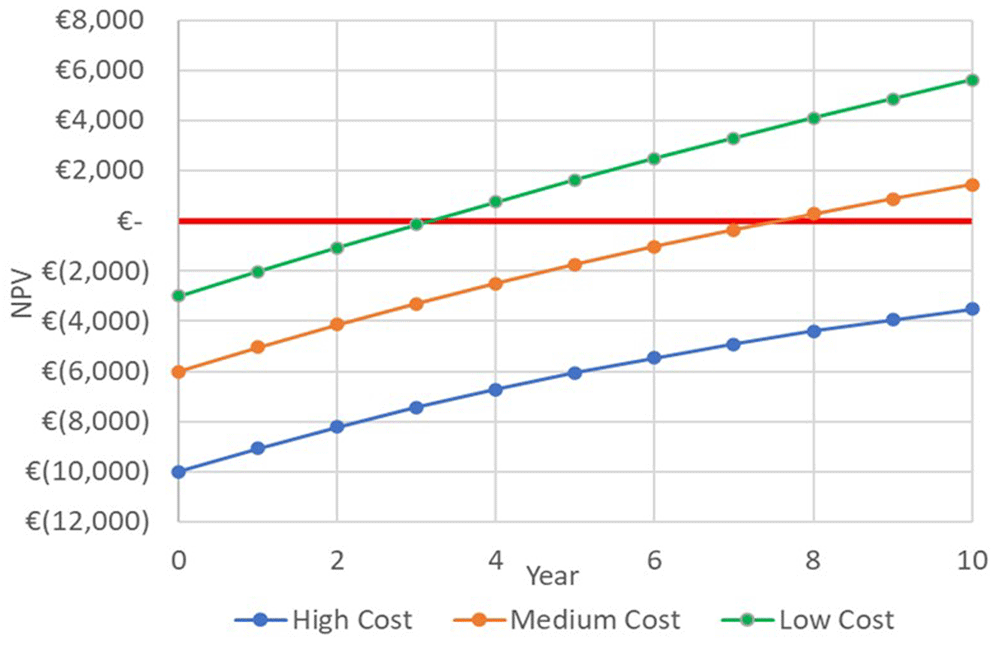
Figure 6. NPV of V2H investment over 10 years under High Cost (investment cost €3000 with 3% discount rate), Medium Cost (investment cost €6000 with 6% discount rate) and Low Cost (investment cost €10000 with 9% discount rate) Scenario cases.
As to the calculations from Equation (15), Figure 7 investigates the DPP under the influence of investment costs by assuming a discount rate of 4% with a 3-tier electricity tariff over a 10-year period. The base case reflects the conditions represented by the origin (0%, 0%) in Figure 5. Apart from the baseline case, there are three additional scenarios investigated in this sector: 1) Scenario I reflects the least favourable household conditions from Figure 5. It assumes a low annual household demand of 2400kWh, 40-kWh EV battery capacity, 54% EV availability and small difference between day and night electricity tariffs; 2) Scenario II reflects the most favourable household conditions for V2H from Figure 5. It assumes the house has a high annual household demand of 9600kWh, 100-kWh EV battery capacity, 95% EV availability and a large difference between day and night electricity tariffs; 3) Scenario III reflects the baseline case with its electricity costs inflated by 5% each year.
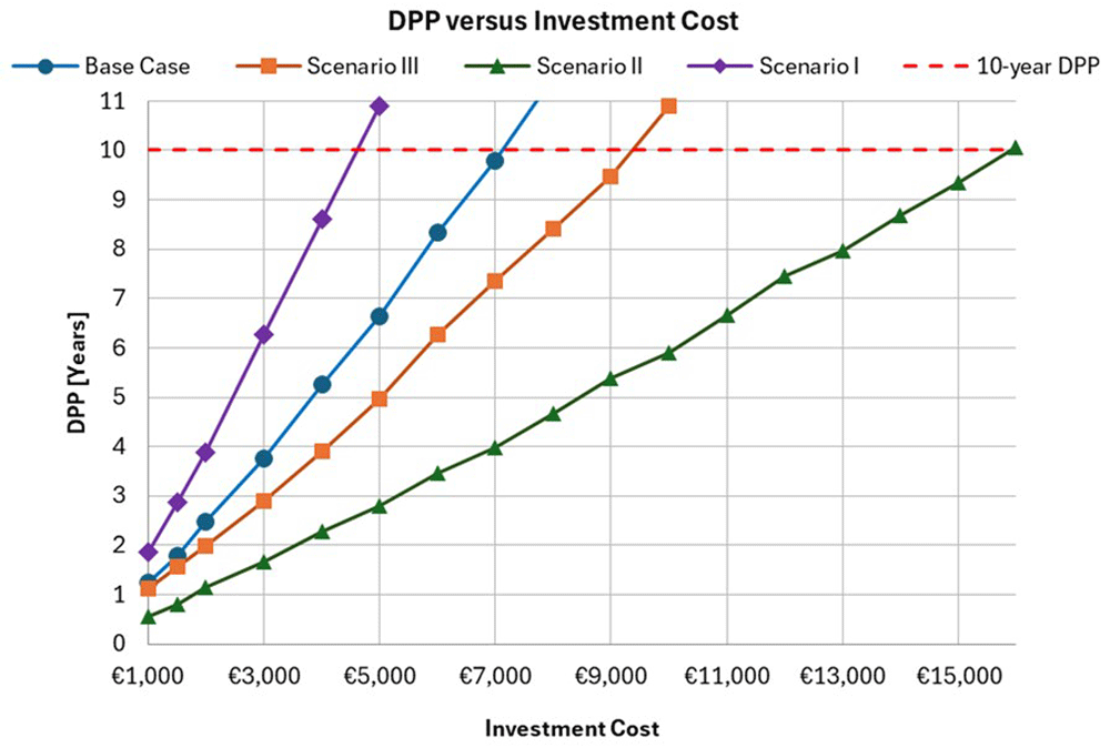
Figure 7. DPP against Investment cost for a variety of household scenarios.
The DPP of baseline case is within 10 years once the investment cost is below €7,000. Scenario I will earn its investment back within a decade if its investment cost is approximately €4,000, whilst for Scenario II, an investment of up to €15,000 would be deemed worthwhile. This is due to the fact that Scenario II has V2H savings of 2038€/a, and by comparison, Scenario I generates V2H savings of merely 98€/a. By considering the 5% inflation in electricity prices each year for the 10-year period under the Scenario III, the maximum investment cost is approximately €9,000 in order to get its payback within a decade. The baseline case could be considered a worthwhile investment as its DPP is below 10 years assuming an initial cost of €7,000 and this maximum investment cost will decrease to €6,000 under a discount rate between 5–7%, and further decline to €5,000 under a discount rate between 8–9%.
Conclusions
This work has presented a V2H optimization model and used it to compare household energy savings from V2H to flexible and uncontrolled charging strategies. The savings from implementing V2H for an average non-commuting user and for an average commuting user in Ireland are found to be 939€/a and 564€/a, respectively resulting in a 30% and 35% overall reduction in household energy costs. These results are consistent with existing literature4,12,29 with the findings of cost savings ranging from 25% to 36%.
According to the sensitivity analysis, the electricity tariff has the greatest impact on V2H cost saving, because a large difference between day and night tariffs results in EV shifting its demand into the night with cheaper prices. Household demand, EV usage and EV availability are proven to be influential on V2H savings too, whilst charging rate and DOD have minimal impact.
Under the 3-tier tariff structure, larger PV capacity has a large impact on percentage energy savings, but minimal impact on the additional savings from V2H, which is in contrast with the findings in Kern et al.12, which found that the V2H cost savings increase with increased PV capacity under the flat tariff. The main reason for this comes from the difference in day and night electricity tariffs. Under a flat tariff there is no preference for shifting the grid demand to the nighttime, unlike the 3-tier tariff structure which makes substantial savings by shifting the grid demands to the nighttime. An increase in PV capacity leads to less grid demand during the day for the 3-tier tariff to shift to the nighttime.
Additionally, in 12 it was found that an average home cannot make a return on their investment of €6000 within 10 years under the flat tariff12. However, by applying the 3-tier tariff structure with a discount rate of 4%, the DPP under an investment cost of €7000 is less than 10 years in this work, due to the cost savings by grid demand shift to preferable low-cost nighttime.
Ethics and consent
Ethical approval and consent were not required.