Shear resistance in high-strength concrete beams without shear reinforcement: A new insight from a structured implementation of Explainable Artificial Intelligence

Masoud Haghbin; María L. Jalón; Natalia Díaz-Rodríguez; Juan Chiachío

doi:10.12688/openreseurope.20195.1

Shear resistance in high-strength concrete beams without shear reinforcement: A new insight from a structured implementation of Explainable Artificial Intelligence

Masoud Haghbin ,
María L. Jalón
,
Natalia Díaz-Rodríguez
,
Juan Chiachío

Article

Authors & roles Authors

Peer review record Peer review

Metrics

Cite

Section

Research Article

Published

April 25, 2025

DOI

https://doi.org/10.12688/openreseurope.20195.1

Versions

April 25, 2025 (Published Manuscript Under Review 1.0)

European Commission

Grant ID(s): 101092052

Views

Downloads

Citations

See full metrics

Shear strength, High-Strength Concrete, Explainable Artificial Intelligence.

Abstract

This paper presents a data-driven modeling methodology based on Explainable Artificial Intelligence (XAI) integrated with Genetic Programming (GP), called XAI-GP, to develop a transparent and practical model for predicting the shear strength of High-Strength Concrete (HSC) beams without shear reinforcement. First, three AI models were trained using empirical data from the literature, and the most accurate model was selected. XAI techniques (SHAP and Breakdown explainers) were then applied in a structured manner to identify key input parameters influencing ultimate shear stress, ensuring model robustness and preventing misleading conclusions. Using these insights, a new shear strength expression was formulated via GP, balancing accuracy, safety, and compliance with design standards. The XAI-GP model was evaluated against empirical models from concrete design codes and previous studies, explicitly considering both safety and accuracy. Results demonstrate that XAI-GP enhances predictive performance while ensuring usability and trustworthiness for engineers.

Corresponding author

Juan Chiachío

jchiachio@ugr.es

Grant information

This work was supported by the Horizon Europe Framework Programme (Grant agreement No. 101092052, BUILDCHAIN: BUILDing knowledge book in the blockCHAIN distributed ledger. Trustworthy building life-cycle knowledge graph for sustainability and energy efficiency).

The funders had no role in study design, data collection and analysis, decision to publish, or preparation of the manuscript.

This work is licensed under a Creative Commons Attribution 4.0 International License.

First version published

April 25, 2025 (https://doi.org/10.12688/openreseurope.20195.1)

Latest version published

April 25, 2025 (https://doi.org/10.12688/openreseurope.20195.1)

1. Introduction

According to the American Concrete Institute, High-Strength Concrete (HSC) is defined as concrete with a specified compressive strength of 55 MPa (8000 psi) or greater¹. This remarkable material has a significant impact on modern structural design due to its superior mechanical performance, including not only higher compressive strength but also long-term durability and higher stiffness, among others^2–4. All tallest buildings and several long-span bridges constructed in the last 20 years have some structural contribution from HSC¹. However, many empirical models used to predict concrete properties or design structural members are based on tests using concrete with compressive strengths lower than 55 MPa¹. The current availability of data for higher strength concretes requires that the models be re-evaluated to determine their applicability to HSC. Therefore, caution should be exercised when extrapolating empirical models from lower to higher strength concretes^1,5. In the particular case of the shear strength, there is general agreement among researchers that the expressions provided in major design codes for the contribution of concrete to shear resistance are conservative for HSC^1,6,7. This conservatism can be seen as beneficial in terms of reliability but unfavorable in terms of sustainability and cost, especially when dealing with tall buildings and long-span bridges. This calls for the need of further research to better represent the actual shear resistance of HSC, which can be distilled into future versions of the design codes.

Over the years, extensive experimental work has been carried out to determine the shear strength of HSC. Zsutty (1968)⁸ pioneered this field of research, proposing prediction models based on data combining dimensional analysis and statistical regression. Following Zsutty’s work, other authors have developed new shear strength models based on their own experiments, offering valuable insights into the various geometry and material parameters influencing the shear resistance of HSC^2,9,10. However, statistical and numerical models have limited validity because they rely on small datasets and simplifications. These models become inadequate to understand the influence of other input parameters not included in the models, or when trying to extrapolate results to different datasets^11,12. In this sense, modern Artificial Intelligence (AI) techniques have become a viable and powerful alternative to exploit the full potential of the existing databases¹³. Recent literature reviews in the context of AI-based modeling of HSC shear strength are found in 11,14. One of the pioneering works in this area is by Cladera and Marí (2004)¹⁵, who developed an Artificial Neural Network (ANN) model for shear resistance in slender beams and, based on a parametric study using the ANN model, they derived a new expression for shear strength in Normal Strength Concrete (NSC) and HSC. In line with this study, subsequent research works have corroborated the superior performance of diverse AI modeling methodologies when compared to conventional models, including those given by the design codes. Some examples can be found in 4,16–19 using ANNs, or using other AI strategies including Genetic Programming (GP)^20–25, Support Vector Regression (SVR)²⁶, Extreme Learning Machine (ELM)^27,28, Model Tree Algorithm 5²⁹, Gradient Boosting Regression Tree (GBRT)³⁰, and Gaussian Process Regression (GPR)³¹, among others. These AI-based models are developed using large databases, leading to higher accuracy, flexibility, and robust generalization capability when fed with other datasets. Nevertheless, the majority of these models suffer from the black-box problem³², being opaque to most end users and therefore increasing the risk of incorrect predictions³³. In this context, recent studies have focused on eXplainable Artificial Intelligence (XAI) techniques¹ to shed light on input parameter contributions to the output of the AI model. This knowledge is crucial for understanding the relative influence of various internal mechanisms governing the shear strength (e.g., aggregate interlock), as represented by input parameters (e.g., maximum aggregate size), on model prediction. The pioneering contribution in this field is by Mangalathu et al. (2020)³⁴, who employed the SHapley Additive exPlanations (SHAP) explainer technique to identify and rank the significant input parameters affecting various failure modes of reinforced concrete columns and shear walls. Their study concluded that geometric input parameters and reinforcement indices are the critical parameters influencing failure modes. In subsequent research, Mangalathu et al. (2021)³⁵ used different AI models such as Ridge Regression (RR), SVR, Decision Tree (DT), K-Nearest Neighbours (KNN), Random Forest (RF), Adaptive Boosting (AB), and eXtreme Gradient Boosting (XGBoost), which were coupled with the SHAP technique to analyze the importance and contribution of the factors that influence the punching shear strength in concrete slabs without transverse reinforcement. They found that the material parameters have a greater influence on the shear strength of flat slabs than the geometric parameters. In line with these pioneering works, other authors have recently adopted the SHAP technique as explainer to understand the role of various parameters in the shear strength in application to deep beams³⁶, flat slabs^37,38 and slender steel fiber-reinforced concrete beams^30,39.

These previous works on XAI have brought a significant advance in the AI modeling of shear resistance with emphasis on the use of SHAP explainer, but they also pose some limitations. A number of these worksare focused on using the SHAP model as a global explainer across the entire dataset^{30,36,41–43}. A major issue with this approach is that although the SHAP explainer is designed to provide explanations both for individual samples as well as at a global model level⁴⁴, it is not elucidating nor representative enough interpreting global model explainers via mean absolute value or any averaging processes of the individual SHAP results⁴⁵. Furthermore, when the SHAP model is applied globally, small changes in the datasets and input distributions can lead to different results and conclusions^45–47. In addition to implementing the SHAP explainer on a global scale based on averaging processes, a few studies also use it as a local explainer. These studies focus explainability analyses on a few samples for the input parameters and provide interpretation results without considering the behavior of the AI model in the vicinity of those points^35,43. A reliable and explainable model should ideally produce similar results around the selected samples. However, most of the cited studies above have overlooked this aspect when using explainer techniques in their analysis. Also, in real case studies, where multiple input parameters with wide ranges of definitions are involved (e.g., compressive strength, shear span, etc.), explainers may behave differently in certain sub-ranges of the inputs⁴⁵. Therefore, focusing the explainability analysis on just a few samples can lead to incomplete or misleading conclusions if the selected points do not cover well the entire range of definitions of parameters.

Lastly, a new current in the XAI field criticizes game theory-based explainability techniques such as SHAP due to their ability to provide features with little actual impact on a prediction—according to SHAP scores—with more importance than features with a meaningful impact on the same prediction⁴⁸. This discrepancy raises concerns about the continued practical use of tools that approximate SHAP scores, especially in high-risk and safety-critical fields. To address these challenges, this paper introduces a three-stage approach called XAI-Genetic Programming (XAI-GP). First, three stacked ensemble AI models for shear strength are obtained based on published datasets^49–53, and the best-performing AI model is selected based on performance metrics. Second, the datasets are clustered based on the compressive strength of concrete $f_{c}^{'}$ , which is a key parameter representing the mechanical behavior of the HSC. This allows for the systematic selection of different samples within each cluster. Then, SHAP and Breakdown (BD) explainers are applied to shed light on the non-linear contribution of each input parameter to the ultimate shear stress results, as predicted by the AI model. Third, based on the results of the explainers in the local stage using multiple samples covering different ranges of the compressive strength of concrete ( $f_{c}^{'}$ ) and genetic feature selection, the most influential parameters are selected to serve as input for a newly generated expression for shear strength using symbolic regression by GP⁵⁴. The overall methodology is demonstrated using a dataset comprising 250 samples of shear strength for HSC slender beams without shear stirrups, gathered from various published sources^49–53. The input parameters considered in this study include the effective depth of the beam (d), the maximum aggregate size (a_g), the width of the beam (b), the shear span (a), the compressive strength of concrete ( $f_{c}^{'}$ ), and the percentage of tension reinforcement (ρ). The results show that ρ and a stand out as the most influential parameters, followed by other input parameters d, $f_{c}^{'}$ , b, and a_g, respectively. Also, it is shown that the newly derived mathematical expression for estimating shear strength demonstrates superior performance compared to existing models in the literature, including those from building standards. This new mathematical expression incorporates a safety factor, which enhances the safety margin, providing more reliability when used for structural design.

The remainder of the paper is organized as follows: Section 2 provides an overview of the mechanism of shear strength in concrete and an overview of the explainable techniques; the methodology to predict the ultimate shear stress of HSC through the explainable AI is discussed in Section 3; the results and discussion are presented in Section 4; finally, conclusions are provided in Section 5.

2. Background

2.1. Overview of shear strength modeling in HSC concrete without transverse reinforcement

According to the literature and the design standards, the shear strength provided by concrete is taken as the shear causing inclined cracking^55–57. After cracking, the shear-transfer actions that contribute to the shear strength of reinforced concrete members without transverse reinforcement are the beam, and the arch actions. The beam mechanism can transfer the shear by the cantilever action, the aggregate interlocking, the residual tensile strength of concrete, and the doweling action of the longitudinal reinforcement bars. With respect to the arch mechanism, the shear is transferred through the inclined compression chord. All these shear-transfer mechanisms ultimately depend on a set of known physical parameters, mainly the concrete compressive strength ( $f_{c}^{'}$ ), the effective depth (d) and width of the beam (b), the shear span (a), the maximum aggregate size (a_g), and the percentage of tension reinforcement (ρ), among others. Nevertheless, there is still no general consensus on the relative importance of these parameters and their associated shear transfer mechanisms in governing the overall shear strength in either NSC or HSC⁵⁸. In particular, it is known that the way in which these mechanisms, and therefore their representative parameters, contribute to the ultimate shear strength varies from one experiment to another, depending on the crack pattern and its kinematics at failure, although the overall shear strength may be similar^59,60. It may also vary from NSC to HSC². This lack of knowledge is also reflected in the design codes, whose provisions for shear design are based on empirical models, which may differ from one code to another, as shown in Table 1. In particular, it is evidenced in Table 1 that two of the most significant building standards codes, namely, ACI-318-19⁶¹ and Eurocode 2 (EN 1992-1-1)⁶², respectively, propose markedly different empirical models for determining the shear strength of concrete beams without shear reinforcement. Moreover, these codes do not distinguish between NSC and HSC, which may result in an underestimation the shear strength of HSC^18,63,64. In contrast, the recently revised Eurocode 2 (FprEN (1992-1-1:2023))⁶⁵ offers a specific expression for shear capacity of beam elements without shear reinforcement in HSC. The same lack of consensus about influential shear transfer mechanisms and the role of their associated parameters is also observed in the literature. For example, Taylor (1970)⁶⁶ proposed that in NSC with a compressive strength between 26 and 49 MPa, the aggregate interlocking, the inclined compression chord, and the doweling action contribute to shear strength within ranges of 33–50%, 20–40%, and 15–25%, respectively. In contrast, in HSC, cracks appear suddenly in a relatively smooth fracture surface^2,67,68, which affect the shear strength of concrete by reducing⁶⁹ or even neglecting⁷⁰ the influence of the aggregate interlock. In this context, Mphonde (1988)⁷¹ proposed that in HSC with a compressive strength between 62 and 90 MPa, the aggregate interlocking, the inclined compression chord, and the doweling action contribute to shear strength within ranges of 0%, 16–26%, and 31–74%, respectively. Regarding modeling, Zsutty (1968)⁸ conducted a pioneering work in this field. He used dimensional analysis and statistical regression methods to propose two models for shear capacity estimation based on the ratio $\frac{a}{d}$ . To this end, he categorized the data based on the $\frac{a}{d}$ values and applied the regression method separately for $\frac{a}{d}$ ≥ 2.5 and $\frac{a}{d}$ < 2.5. This categorization of data was useful because samples with $\frac{a}{d}$ ≥ 2.5 were influenced by beam action, while those with $\frac{a}{d}$ < 2.5 were influenced by arch action. Several attempts to refine and build upon the Zsutty (1968)⁸ work have arisen in the literature to improve the existing shear capacity models^{49,70,72–74}. In particular, Hamrat et al. (2010)² conducted a study using video recording and laboratory experiments to investigate the role of ρ, $\frac{a}{d}$ and $f_{c}^{'}$ on specimens. They found that most building code models perform well when a/d ≥ 2 and that shear capacity depends more on the shear-span/depth ratio ( $\frac{a}{d}$ ) and the longitudinal steel ratio (ρ) and relatively less so on the compressive strength ( $f_{c}^{'}$ ) in the case of HSC. In addition to these valuable insights about the influence of factors on shear capacity, they suggested a new model generated by multiple linear regression analysis that can be used for both NSC and HSC samples. In line with previous studies, a subsequent research effort was carried out by El-sanadedy et al. (2016)⁴. They utilized their sensitivity analysis findings, obtained via ANN, to derive a model for shear capacity that outperforms other models. In 2022, the European Committee for Standardization published a new version of the Eurocode (FprEN (1992-1-1:2023))⁶⁵ for concrete structures, which includes several modifications to the shear capacity model, particularly regarding the impact of aggregate size. The new model proposed by the Eurocode (FprEN (1992-1-1:2023)), along with the previously discussed models, is summarized in Table 1 and is further compared with the model proposed in this study.

Table 1. The suggested models exist in the literature to estimate shear strength.

Author	Model	Description
ACI-318-19⁶¹	$V = 0.11 λ \sqrt{f_{c}^{'}} b d$	λ: modification factor $f_{c}^{'}$ : compressive strength of concrete b: width of the beam d: depth of the beam
Eurocode 2 (EN 1992-1-1)⁶²	$V = [C_{R d, c} k {(100 ρ f_{c}^{'})}^{\frac{1}{3}}] b d$	C_Rd,c: safety coefficient, C_Rd,c = $\frac{0.18}{γ_{c}}$ γ_c: partial safety factor k: size effect coefficient, k = 1 + $\sqrt{\frac{200}{d}}$ ≤ 2.0 with d in mm ρ: tension reinforcement ratio, ρ = $\frac{A_{s}}{b d}$ ≤ 0.02 A_s: area of tensile reinforcement
FprEN (EN 1992-1:2022)⁶⁵	$V = \frac{0.66}{γ_{v}} {(100 ρ f_{c}^{'} \frac{d_{d g}}{d})}^{\frac{1}{3}} (b d)$	d_dg: failure zone property d_dg = 16mm + D_lower ≤ 40mm for $f_{c}^{'}$ ≤ 60 MPa d_dg = 16mm + D_lower ${(\frac{60}{f_{c}^{'}})}^{2}$ ≤ 40 mm for $f_{c}^{'}$ ≥ 60 MPa D_lower: smallest sieve size in aggregate γ_v: safety factor
El-sanadadey et al. (2016)⁴	$V = 0.73 {(f_{c}^{'})}^{0.18} {(\frac{a}{d})}^{- 0.62} {(\frac{27500 ρ}{d})}^{0.45} b d$	a: shear span ρ: tension reinforcement ratio, ρ = $\frac{A_{s}}{b d}$
Hamrat et al. (2010)²	$V = 3.88 {({f^{'}}_{c} ρ \frac{d}{a})}^{0.47} b d (\frac{a}{d} < 2.5)$ $V = 2.40 {({f^{'}}_{c} ρ \frac{d}{a})}^{0.41} b d (\frac{a}{d} \geq 2.5)$
Cladera and Marí (2004)⁷²	$V = 0.225 ξ 100 ρ^{\frac{1}{2}} f_{c}^{' 0.2} b d$	ξ: size effect coefficient, ξ = 1 + ${(\frac{200}{s_{x}})}^{0.5}$ = 2.75 s_x: mechanical depth, s_x = 0.9d
Zsutty (1968)⁸	$V = 2.2 {(\frac{f_{c}^{'} ρ d}{a})}^{1 / 3} b d (\frac{a}{d} \geq 2.5)$ $V = 5.1 (\frac{d}{a}) {(\frac{f_{c}^{'} ρ d}{a})}^{1 / 3} b d (\frac{a}{d} < 2.5)$

From observation of Table 1, it is evident that although different models account for different governing shear-carrying actions in different ways, the final expressions account for similar parameters with similar influences and, in most cases, fit in a similar manner compared to available datasets⁵⁸.

2.2. Overview of eXplainable Artificial Intelligence techniques

This section briefly explains the eXplainable Artificial Intelligence (XAI) techniques adopted in this research to unveil the subtle contributions of the various input parameters in the prediction of the ultimate shear stress. Explainability techniques attempt to clarify the consistency of AI models’ prediction and the influence of each input parameter on the AI model’s results^75,76. This valuable information is further used in this study to propose an alternative expression for shear strength in HSC based on the most influential parameters as identified by XAI.

In this research, SHapley Additive exPlanations (SHAP) and the Breakdown (BD) techniques have been selected for their robustness and efficiency⁷⁷. The SHAP model is based on game theory, while BD is based on the greedy approximation approach. Also, these methods are frequently used in the XAI community, offering flexibility, model-agnostic features, and data independence⁷⁸. Validating results with this dual approach highlights potential discrepancies, reinforces interpretation stability, and provides a well-rounded understanding of feature importance. BD works by decomposing the AI model’s prediction into different parts based on the contributions of the specific input parameters. Mathematically; this decomposing is achieved using a scoring function, which is expressed as a linear combination of the input parameters. In this explainer, the contributions of each input parameter are sequentially added to a baseline prediction (intercept) until the total prediction of the AI model is fully explained⁷⁹. The scoring function is expressed mathematically as follows:

F (x^{new}) = (1, x^{new}) {(μ, β)}^{T} = μ + x_{1}^{new} β_{1} + \dots + x_{p}^{new} β_{p} (1)

where F(x^new) is the model prediction (ultimate shear stress in this case) for x^new = $[x_{1}^{new}, x_{2}^{new}, . . ., x_{p}^{new}],$ , where $x_{i}^{new}$ , i = 1,2, . . . , p represents one of the input parameters used in this work, including ρ, b, d, a, a_g, and $f_{c}^{'}$ ; µ is the intercept that refers to the model prediction when input parameters are set to their reference values (e.g., mean, median, or when all x^new are zero); and β = [β₁, β₂, ..., β_p] refers to the weights assigned to each independent input parameter. A detailed description of the BD technique is available in 79.

On the other hand, SHAP is a technique inspired by game theory⁸⁰ where the contribution of each input parameter on the predicted results (v) by the AI model is obtained based on their marginal contribution^81,82. To this end, SHAP employs an additive feature attribution method to find the contribution of each input parameter to the predictions³⁴, which is expressed as follows:

g (z^{'}) = ϕ_{0} + \sum_{i = 1}^{n} ϕ_{i} {z^{'}}_{i} (2)

where ź is a binary vector of input parameters, $z_{i}^{'}$ is zero when an input parameter is not observed; otherwise, it is 1; n denotes the number of input parameters, ϕ₀ is a constant value that represents the model’s prediction in the absence of any input parameters or when all input parameters are zero. Since tree-based models such as Gradient Boosted Machines (GBM) and RF are used in this research as prediction models, ϕ₀ is defined similarly to the intercept term (µ) in Equation (1) and ϕ_i is the assigned weight or contribution of input parameter i on model’s predictions (val), which can be calculated as follows:

ϕ_{i} (v a l) = \sum_{S \subseteq {1, . . ., p} \ {i}} \frac{| S |! (p - | S | - 1)!}{p!} (v a l (S \cup {i}) - v a l (S)) (3)

where S represents the subsets of all input parameters excluding feature i, p denotes the total number of input parameters, and |S| refers to the number of elements (cardinality) in subset S. The term p! represents the factorial of the total number of features, accounting for all possible feature orderings. The function val(S ∪ {j}) denotes the model’s prediction when using the features in subset S along with feature i, while val(S) denotes the model’s prediction when using only the features in subset S. The fraction $\frac{| S |! (p - | S | - 1)!}{p!}$ is a weighting factor that ensures a fair distribution of feature contributions across all possible subsets. Equation (3) sums the effects of all input parameters on the predictions made by the AI model. More details about SHAP analysis can be found in 44,80.

3. Methodology

This study presents a multi-step approach referred to as XAI-GP for predicting shear strength. First, open-source datasets from the literature^49–53 were collected, and input parameters (b, d, a, a_g, $f_{c}^{'}$ , ρ) were selected to provide a comprehensive representation of the problem. Then, three candidate AI-based models are trained using gathered datasets, and the most accurate model is selected based on performance metrics. In the next step, the datasets are grouped based on the $f_{c}^{'}$ values, and SHAP and BD explainers are employed to analyze how input parameters non-linearly influence ultimate shear stress predictions. As an outcome, the most influential parameters are identified through explainers and genetic feature selection, considering data from various compressive strength groups. This process allows for discovering a new shear strength model using symbolic regression with GP based on the most influential input parameters. A safety factor is then determined and incorporated into the new model to ensure the safety of the proposed model for end-users. Finally, the new model is compared with existing models in literature and design standards, and it is validated using additional external datasets to evaluate its performance. Figure 1 shows a flow chart of the different stages of the proposed methodology.

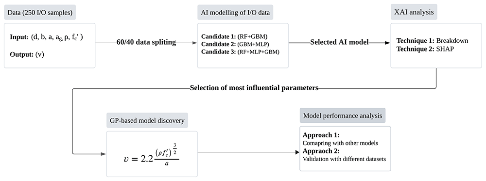
Figure 1. Scheme of the proposed methodology to generate a mathematical expression.

In regards to the AI modeling of the I/O data, this research used a stacked ensemble approach to estimate ultimate shear stress (output) based on the input data. This approach minimizes overfitting and reduces the generalization error in regression tasks. This study proposes three stacked ensemble models as predictor candidates by integrating different base learners. RF, GBM, and MLP are adopted as base learners to capture various patterns in the dataset. Stacked ensemble 1 is obtained by combining RF + GBM; stacked ensemble 2 is based on GBM + MLP; stacked ensemble 3 is obtained as RF + GBM + MLP. Base learner RF reduces variance through an ensemble approach⁸³, while GBM is used to adapt better to our datasets with mixed features in an efficient manner⁸⁴. Lastly, MLP has the ability to model non-linear relationships within the dataset⁸⁵. The meta-learner (GBM) was trained on the outputs from the base learners, effectively combining their outputs to maximize their strengths. This choice resulted in a significant performance improvement compared to any single model.

To find the best-performing stacked ensemble AI model, performance metrics such as the coefficient of determination (R²), the Root Mean Square Error (RMSE), and the Mean Absolute Error (MAE) are calculated in both training and test stages. Subsequently, as explained before, the effect of the input parameters on the results generated by the most effective AI model is examined using XAI techniques detailed in Section 2.2. The XAI analysis was conducted using DALEX⁸⁶, DALEXtra⁸⁷, and H2O⁸⁸ packages in R software. To this end, 15 I/O samples are selected so that they represent different ranges of $f_{c}^{'}$ using the univariate k-means clustering method⁸⁹. These samples are utilized as representatives to carry out the XAI analyses. Finally, a new mathematical expression to calculate the shear strength is obtained through GP modeling, using most important input parameters obtained from the explainer techniques and genetic feature selection.

GP is inspired by the principles of natural selection and genetics. Similar to Genetic Algorithms (GA)⁹⁰, the GP model uses genetic operators such as crossover, mutation, and selection integrated into a tree-structure approach to produce a symbolic model that contains mathematical operators such as +, −, ×, log to represent the relationship between input and output parameters in a dataset. In the GP modeling process, each generation of individuals is evaluated using a fitness function, such as Mean Squared Error (MSE), with higher-scoring individuals more likely to be selected for reproduction. Reproduction involves crossover, where segments from two parents are combined, and mutation, which, introduces random changes to improve individuals. Over successive generations, the population evolves, gradually improving solutions based on the fitness function. This process continues until a stopping criterion is met, such as reaching a target fitness level or completing a specified number of generations.

4. Results and discussion

4.1. Description of the data set

The methodology proposed in this paper is illustrated here for a data set from open-access literature about HSC slender beams longitudinally reinforced without shear stirrups⁴. This data set is composed of 250 samples that have reached shear failure during the experiments. It is randomly split into training and testing subsets with a 60/40 ratio. The samples are defined by the following input parameters: effective depth of the beam (d), the maximum aggregate size (a_g), the width of the beam (b), shear span (a), compressive strength of concrete ( $f_{c}^{'}$ ), and percentage of tension reinforcement (ρ); the output is the ultimate shear stress (v). Figure 2 represents the histograms of the input and output parameters to visualize the relative variability of such data.

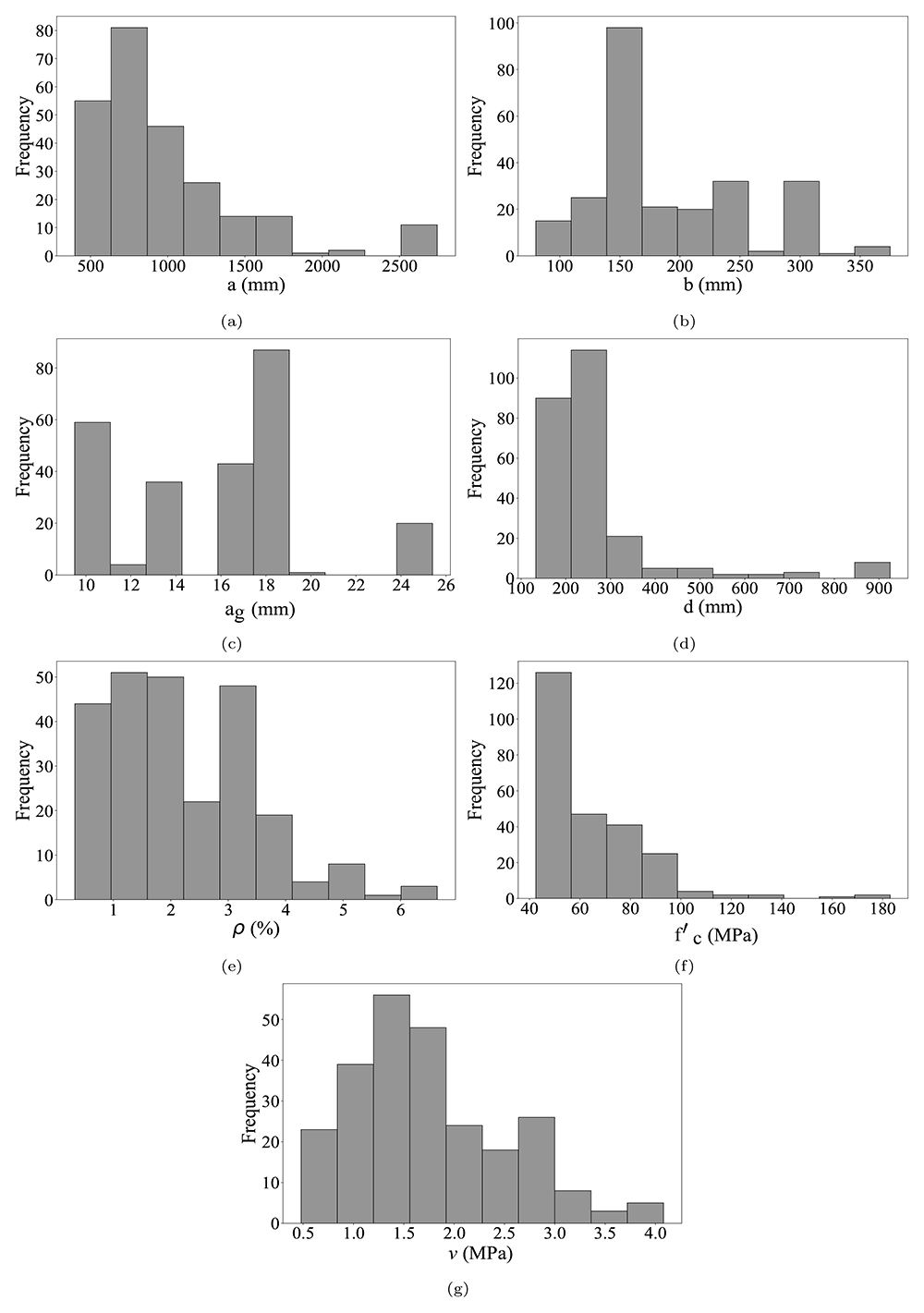
Figure 2.

Histograms of the input parameters in the dataset: (a) shear span (mm), (b) width of the beam (mm), (c) maximum aggregate size (mm), (d) effective depth of the beam (mm), (e) the percentage of tension reinforcement (%) (f) compressive strength of concrete (MPa), (g) ultimate shear stress (MPa).

4.2. AI model selection

In this section, the performance of each stacked ensemble model as defined in Section 3 is evaluated and compared using different performance metrics such as R², RMSE, and MAE. Then, the model with the best performance is selected based on these metrics. Table 2 presents the results for various AI models during both the training and testing stages.

Table 2. Performance metrics of different AI models and different training and testing stages.

Train Stage
Model Name	RMSE	R²	MAE
Stacked ensemble 1	0.158	0.960	0.101
Stacked ensemble 2	0.147	0.964	0.094
Stacked ensemble 3	0.158	0.965	0.095
Test Stage
Stacked ensemble 1	0.290	0.841	0.201
Stacked ensemble 2	0.297	0.834	0.212
Stacked ensemble 3	0.286	0.845	0.200

As it can be observed from Table 2, the stacked ensemble models generate reliable results at both the training and the test stages, however, stacked ensemble model 3 is the best-performing AI model. In this sense, all the results presented henceforth are calculated for this selected AI model.

4.3. Explainable Artificial Intelligence techniques

The BD and SHAP techniques, as discussed in Section 2.2, are applied to the stacked ensemble 3 using different samples. To select samples, the uni-variate k-means clustering was applied to segment data based on the $f_{c}^{'}$ , identifying four distinct clusters according to the Bayesian Information Criterion (BIC)⁸⁹. The specified values of $f_{c}^{'}$ in each cluster are adjusted to comply with international building standards. The $f_{c}^{'}$ is divided into four clusters. Cluster 1 encompasses strengths ranging from 35 to 55 MPa. Cluster 2 covers strengths from 55 to 75 MPa. Cluster 3 ranges from 75 to 120 MPa, and Cluster 4 has strengths greater than 120 MPa. This clustering allowed identifying a group of similar samples to efficiently analyze the explainers’ performances based on reflecting mechanical characteristics. Table 3 details the selected samples and their associated clusters.

Table 3. Selected samples for the explainer techniques (input parameters: d, b, a_g, $f_{c}^{'}$ , a; output parameter: v).

Sample (Cluster)	d (mm)	a (mm)	a_g (mm)	$f_{c}^{'}$ (MPa)	ρ (%)	b (mm)	v (MPa)
1 (Cluster 1)	278	812	19	50.10	1.57	360	1.19
2 (Cluster 1)	230	805	9.5	50.70	3.10	160	1.73
3 (Cluster 1)	267	1334	19	50.10	0.87	152	1.03
4 (Cluster 2)	208	562	12.7	66.30	2.25	127	3.03
5 (Cluster 2)	202	807	12.7	66.30	5.04	127	2
6 (Cluster 2)	359	1081	12	66.50	2.24	200	1.39
7 (Cluster 2)	202	545	12.7	66.30	5.04	127	3.91
8 (Cluster 2)	202	605	12.7	66.30	5.04	127	2.69
9 (Cluster 2)	465	1600	9.5	66	1	135	0.86
10 (Cluster 2)	208	624	12.7	66.30	2.25	127	1.77
11 (Cluster 3)	925	2664	10	91.60	0.51	300	0.60
12 (Cluster 3)	208	549	18	90	0.74	262	1.39
13 (Cluster 3)	718	2628	16	91.30	1.72	300	1.20
14 (Cluster 3)	690	2629	16	91.70	3.57	300	1.85
15 (Cluster 4)	250	1000	19	183	3.04	200	2.11

Figure 3 illustrates the BD profile for sample 1. The first row, denoting the intercept, displays the mean value of the predicted ultimate shear stress (v_predicted) using all test samples (e.g., sample 1 to 15). The last row, denoting the prediction and representing by a purple bar, shows the predicted ultimate shear stress (v_predicted) specifically for the selected sample (e.g., sample 1). Between these rows are representations of predictions where each input parameter is sequentially fixed one by one, while the other input parameters are allowed to vary, as illustrated by vertical lines. Here, pink bars indicate a negative impact (i.e., a decrease in the prediction value), while green bars signify a positive impact (i.e., an increase in the prediction value). The numerical values next to the pink and purple bars provide insights into the magnitude of these impacts. Furthermore, the x-axis portrays the model prediction value, while the y-axis displays the input parameters and their values for the observation. Finally, the input parameters and their contribution values are listed, starting with the one that has the highest relative importance on the y-axis.

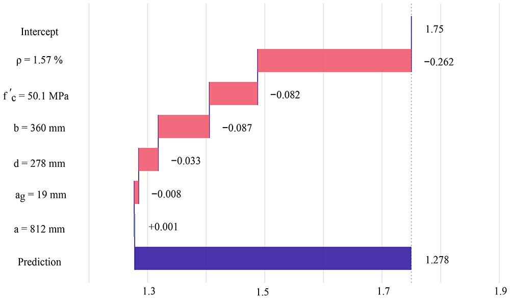
Figure 3. Breakdown (BD) profile for sample 1.

For instance, it can be observed from Figure 3 that the contribution value of each input parameter on prediction (v = 1.278MPa), based on intercept value (v_predicted=1.75 MPa) for ρ, $f_{c}^{'}$ , b, d, a_g, and a, is -0.262, -0.082, -0.087, -0.033,-0.008 and +0.001, respectively. This highlights the relative importance of each explanatory input parameter, denoted by its rank: ρ (1^st rank), $f_{c}^{'}$ (2^nd rank), b (3^rd rank), d (4^th rank), a_g (5^th rank), and a (6^th rank). Finally, it is notable that BD profiles and the rank of each input parameter vary among the different selected samples. Additional details for the BD results of other samples can be found in Appendix A.1. Additionally, Figure 4 represents the SHAP profile for selected sample 1 and visualizes the contribution of each input parameter based on the mean attribution values. The blue box plots summarize the distribution of the attributions for each input parameter across its ranking. The red and green bars display the SHAP contribution values and their negative and positive impacts, respectively. The x-axis portrays the contribution and the y-axis shows the input parameters and their values for the observation. Like the BD profile, the input parameters are written starting with the one with higher relative importance.

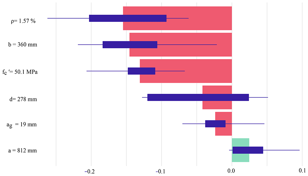
Figure 4. SHAP profile with the average contributions for 25 random orderings using the sample 1.

Figure 4 indicates that ρ (1^st rank) and a (6^th rank) played the most and least important roles in estimating v in the selected sample 1, aligned with the BD technique results (see Figure 3). To obtain the contribution of each feature, SHAP values were calculated 25 times with different feature orderings and averaged to provide a more reliable estimate. It is worth noting that similar to BD profiles, SHAP profiles reveal the variability in the rank of each input parameter across different samples. Additional details for the SHAP results of other samples can be found in Appendix A.2.

The ranking of each input parameter in each sample using the BD and SHAP techniques is depicted in Figure 5. As observed, the ranks of input parameters a (Figure 5a) and ρ (Figure 5e) exhibit close similarity between BD and SHAP techniques, with the highest ranks being 1^st or 2^nd. Figures 5b, 5d, and 5c present the comparison between both XAI models for b, d, and $f_{c}^{'}$ , respectively. These figures illustrate that these input parameters are normally ranked between 3 and 5, with minimal differences in both techniques across most samples. One notable discovery of this study is the significance of maximum aggregate size (a_g) in both explainer techniques. As evident from Figure 5c, the ranks of a_g are almost placed last in both BD and SHAP profiles. These findings are consistent with previous literature⁶⁹ which suggests that in HSC, aggregate interlocking becomes less significant as cracks do not propagate around aggregate particles^66,71.

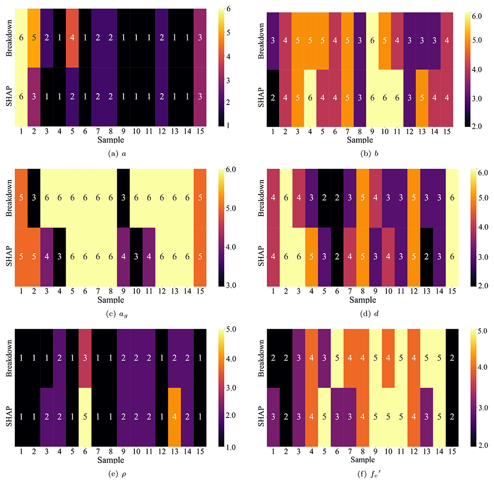
Figure 5.

Rankings (1 to 6) across each of the 15 samples, employing both the BD and SHAP XAI techniques, considering various input parameters: (a) shear span (mm), (b) width of the beam (mm), (c) maximum aggregate size (mm), (d) effective depth of the beam (mm), (e) percentage of tension reinforcement (%), and (f) compressive strength of concrete (MPa).

Finally, the selection of the most important input parameters is determined by attaining lower or higher mode values across both models. Through mode analysis, ρ, a, d, $f_{c}^{'}$ , b, and a_g are ranked as the most to least important input parameters, respectively for both XAI approaches. This ranking aligns with prior research findings⁴.

To assess the robustness of the explainer models, the runs are replicated nine times for each sample to evaluate the variation in explanation outputs across different runs. This approach aids in understanding the sensitivity of the results. In several replications, ρ, a, and $f_{c}^{'}$ were consistently identified as the most important parameters in both SHAP and BD. Other input parameters exhibited similar variations as shown in Figure 5. In addition, different datasets^63,91,92 are used to assess the consistency of the explainers further, providing a comprehensive evaluation of their generalization. The analysis revealed that ρ, a, $f_{c}^{'}$ , and d were the most influential factors compared to b and a_g.

The results from these additional runs and evaluations are included in Appendix B, offering more pro-found insights into the stability and reliability of the explainer models across diverse conditions. Finally, to evaluate the consistency of the performance of both explainers in almost similar samples (those in the same cluster), a mode analysis of the rank positions of each parameter was carried out separately for each cluster, as visualized in Figure 6.

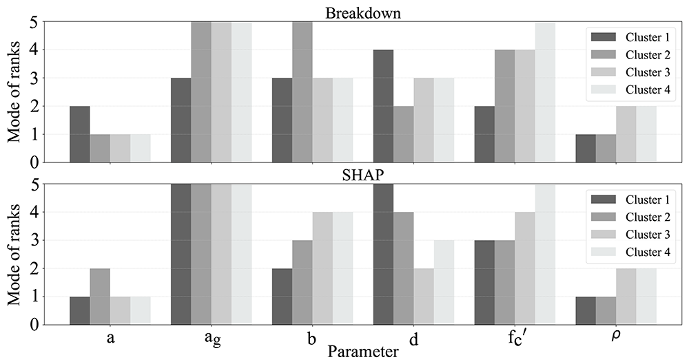
Figure 6. Mode analysis of rank positions for model parameters using Breakdown and SHAP explainers across different clusters.

Figure 6 clearly shows that the rankings of each input parameter can vary across different ranges of $f_{c}^{'}$ . This suggests that the importance of each input parameter is not static across the entire dataset but varies depending on the range of $f_{c}^{'}$ and the specific samples being analyzed. Furthermore, increasing the number of input parameters can further increase this fluctuation, which is common in real case studies. This variation also raises questions about the reliability of using SHAP as a global explainer, particularly in datasets sourced from diverse resources, since a global SHAP explainer relies on the mean absolute of such variable SHAP values.

The approach proposed in this study involves using explainer techniques on a local scale and different clusters and increasing the number of samples instead of using a global scale to address the mentioned issues. This approach allows for a more specific analysis of the importance of input parameters within each group.

One of the benefits of the proposed approach is presenting detailed information to structural engineers without an AI background, who are required to understand the precise impact of input parameters on predictions at a local level, for instance, specific concrete beam samples. This requirement has not been fully covered in earlier investigations, in which the authors tend to visualize SHAP value dependency plots against input parameters.

4.4. Proposing a model based on XAI input parameter selection and GP

In this section, a new mathematical expression is proposed to calculate the shear strength V, derived from GP and focused on the importance of input parameters obtained in Section 4.3. To do this, first, the ultimate shear stress (v) is derived through a GP model utilizing the open-source Python package gplearn⁹³ and based on training data, which are available in a GitHub repository. To train the GP, a 60/40 train-test ratio similar to Section 4.2 was used. GP was limited to using only basic mathematical operators: power, multiplication (×), cube root $(\sqrt[3]{x})$ , square root ( $\sqrt{x}$ ), and division (/) to ensure that the mathematical operators used by GP were aligned with those found in standard design codes to maintain compliance. In addition, the depth of the tree structure was limited to 5 and the length to 10 to generate a short and fairly accurate model. In this research, the most critical input parameters were identified as ρ, a, d, and $f_{c}^{'}$ . Then, the genetic feature selection was activated to simplify the model while achieving similar results with fewer terms. This process leads to the following equation for calculating v:

v = 2.2 \frac{{(ρ f_{c}^{'})}^{\frac{3}{2}}}{a} (4)

where a represents the shear span in mm, ρ stands the percentage of tension reinforcement (non-dimensional) and $f_{c}^{'}$ denotes the compressive strength of concrete in MPa.

Furthermore, the shear strength values as given by GP, denoted as (V₀), are obtained using Equation (4) as follows:

V_{0} = 2.2 \frac{{(ρ f_{c}^{'})}^{\frac{3}{2}}}{a} b d (5)

To address material and loading uncertainties, a Safety Factor (SF) was applied to Equation (5) in order to obtain the design shear strength, denoted as V, as follows:

V = \frac{2.2}{S F} \frac{{(ρ f_{c}^{'})}^{\frac{3}{2}}}{a} b d (6)

To determine the safety factor (SF), the ratio V₀/V_data was calculated for each sample, and the median was obtained, giving a value SF = 1.34. The median was selected because it provides a robust measure of central tendency, effectively minimizing the influence of outliers or extreme values in the data. Finally, Equation (5) and Equation (6) were compared with empirical models commonly found in structural engineering standards and previous studies. These include ACI-318-19⁶¹, Eurocode 2 (EN 1992-1-1)⁶², revised Eurocode 2 (named as FprEN (1992-1-1:2023))⁶⁵, El-sanadadey⁴, Hamrat², Zsutty⁸ and Cladera and Marí¹⁵. The corresponding models are referenced in Table 1. The utilized dataset corresponds to the data employed during the testing stage of GP. However, certain samples were omitted to ensure conformity with the specified range recommended by the standards. (e.g., $f_{c}^{'}$ ≤ 80 MPa).

Figure 7 shows the experimental shear strength (V_data) plotted against the calculated shear strength (V_calculated) using different models, including XAI-GP (Figures 7a and 7b), Cladera and Marí (Figure 7c), ACI-318-19 (Figure 7d), Eurocode2 (EN 1992-1-1) (Figure 7e), FprEN (1992-1-1:2023) (Figure 7f), El-sanadadey (Figure 7g), Hamrat (Figure 7h), and Zsutty (Figure 7i) (see Table 1). It is clear from Figure 7a that most of the samples fed to the XAI-GP model are closer to the perfect fit line when compared to samples from other mathematical expressions.

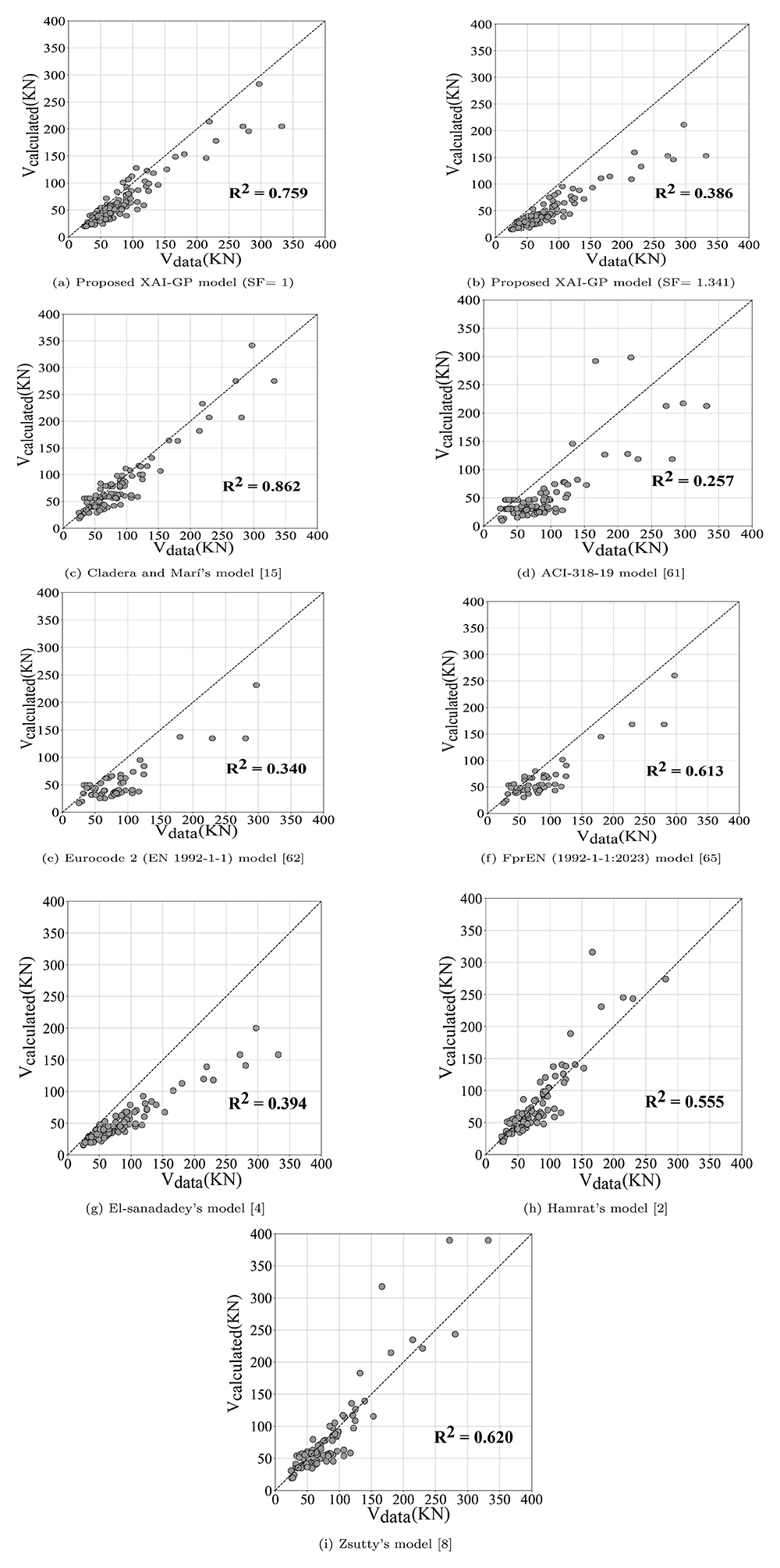
Figure 7. Experimental shear strength plotted against calculated shear strength with test data.

This superior performance of the proposed model is also reflected in the performance metrics calculated and shown in Table 4. To ensure a fair comparison between models, the level of safety provided by the model should be considered in addition to accuracy. To this end, a new metric called the Accuracy-Weighted Safety Score (AWSS) is designed. First, a penalty factor is calculated based on the relative number of overestimated samples (the ones that are above the perfect fit line (diagonal black dashed lines in Figure 7)) over the total samples, referred to as the Degree of Safety (DoS). The DoS is obtained as $1 - \frac{N_{o v e r}}{N_{t o t a l}}$ , where N_over represents the number of overestimated data points calculated by the model, and N_total indicates the total number of data points. The range of DoS is from 0 to 1, where 1 indicates maximum conservativeness and safety, whereas 0 indicates the opposite. This DoS value is then multiplied by R² to obtain the AWSS, presented in Table 4. Therefore, the AWSS ranges from 0 to 1, giving higher values to models with relatively high accuracy R² and safety (DoS). Oppositely, low AWSS values will be attributed to models given relatively low values for accuracy and/or safety. According to the performance metrics, the newly proposed model outperforms the standard codes (ACI-318-19, FprEN (1992-1-1:2023), Eurocode 2 (EN 1992-1-1)) and empirical models by Zsutty, Hamrat, and El-sanadadey. Although the results from Cladera and Marí’s model were slightly better than the proposed model in this study (Equation (5)), the proposed one is simpler and more conservative.

Table 4. Performance metrics of different models to estimate shear strength with test data.

Model	RMSE (KN)	MAE (KN)	R²	DoS	AWSS
XAI-GP (SF=1)	28.57	21.29	0.759	0.84	0.638
XAI-GP (SF=1.34)	45.72	36.39	0.385	1	0.386
Cladera and Mar´¹⁵	21.65	15.97	0.862	0.79	0.681
ACI-318-19⁶¹	50.01	41.20	0.257	0.231	0.90
Eurocode 2 (EN 1992-1-1)⁶²	43.44	34.37	0.340	0.72	0.245
FprEN (1992-1-1:2023)⁶⁵	33.29	25.86	0.613	0.84	0.514
El-sanadadey⁴	45.33	35.01	0.394	1	0.394
Hamrat²	38.89	20.69	0.555	0.56	0.310
Zsutty⁸	38.89	20.71	0.620	0.65	0.403

4.4.1. Model validation with a different dataset. To ensure the robustness and generalization ability of the proposed model, a verification process was conducted using additional datasets presented by 63,91,92. These datasets encompass 31 HSC samples with $f_{c}^{'}$ ranging from 50.5 MPa to 83.4 MPa, ρ fluctuating from 0.35% to 6.64%, a ranging from 450 mm to 851 mm, b varying from 100 mm to 200 mm, d ranging from 150 mm to 250 mm, and V_data ranging from 13.3 kN to 83.4 kN. To ensure a fair comparison, samples outside the recommended ranges for $f_{c}^{'}$ as specified by standard codes such as ACI-318-19⁶¹, FprEN (1992-1-1:2023)⁶⁵, and Eurocode 2 (EN 1992-1-1)⁶², as well as those based on empirical models by Zsutty, Hamrat, and El-Sanadadey, were excluded of the analysis. The results of comparative analysis with these new datasets are visualized in Figure 8.

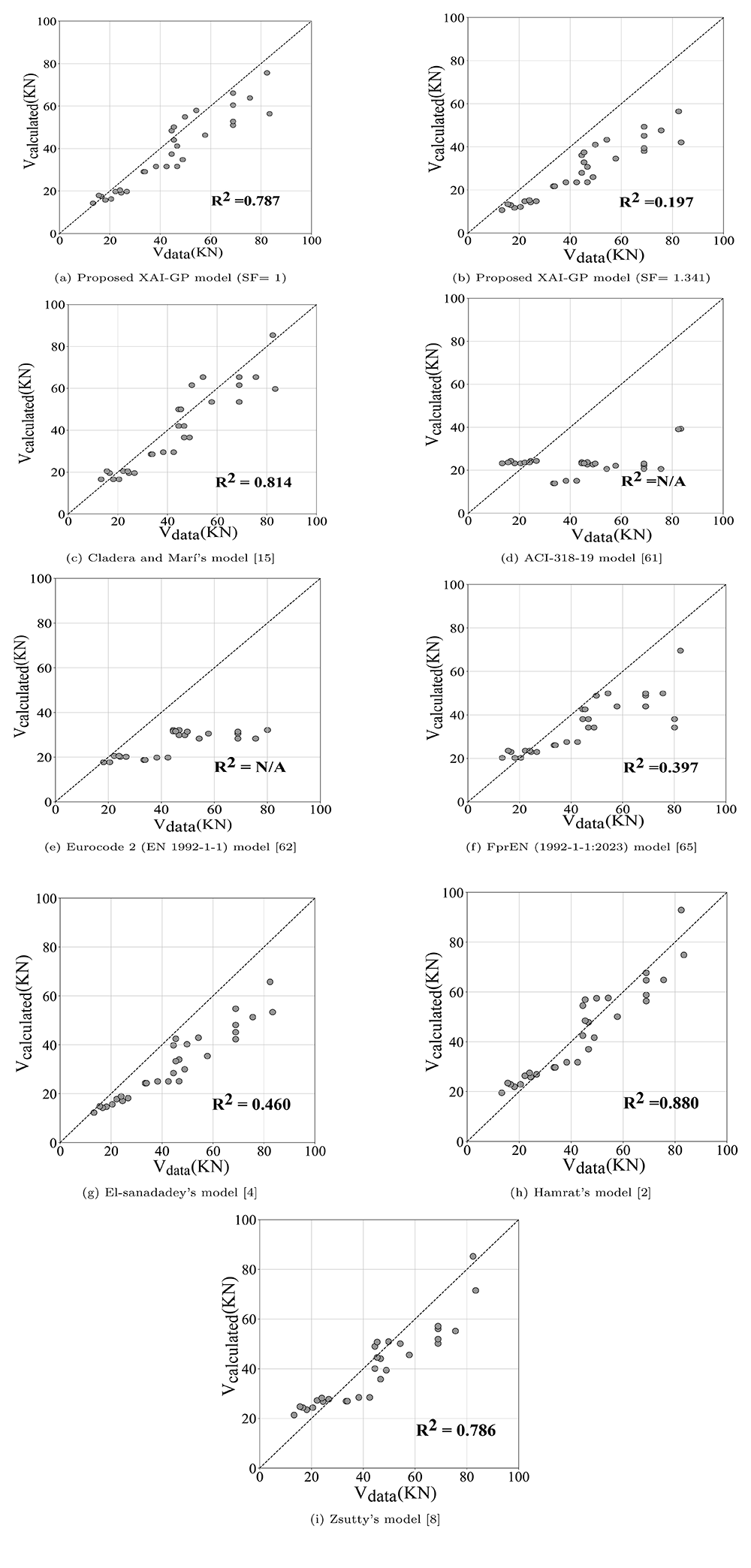
Figure 8. Experimental shear strength plotted against calculated shear strength with verification data.

The performance metrics were calculated similarly to Section 4.4, which are shown in Table 5.

Table 5. Verification of the proposed model with other datasets.

Model	RMSE (KN)	MAE (KN)	R²	DoS	AWSS
XAI-GP (SF=1)	9.35	7.293	0.787	0.766	0.604
XAI-GP (SF=1.34)	18.19	15.65	0.198	1	0.198
Cladera and Mar´¹⁵	8.75	7.20	0.814	0.700	0.570
ACI-318-19⁶¹	23.78	28.37	N/A	0.800	N/A
Eurocode 2 (EN 1992-1-1)⁶²	24.21	19.81	N/A	1	N/A
FprEN (1992-1-1:2023)⁶⁵	16.13	11.49	0.397	0.830	0.333
El-sanadadey⁴	14.94	12.55	0.460	1	0.460
Hamrat²	7.02	6.06	0.880	0.466	0.411
Zsutty⁸	9.38	7.83	0.786	0.566	0.445

Based on the results obtained, the proposed model (Equation (5)) yields the maximum AWSS value of 0.604, which indicates the healthiest balance between accuracy and conservativeness compared to other models. Cladera and Marí’s model¹⁵ ranked second with an AWSS value of 0.577. Despite its high level of accuracy, it has resulted in relatively lower DoS values compared to the proposed model Equation (5). Regarding the standard codes, FprEN (1992-1-1:2023)⁶⁵ outperformed other standard codes such as ACI-318-19⁶¹ and Eurocode 2 (EN 1992-1-1)⁶², based on the AWSS value. This standard demonstrated better accuracy and a higher level of DoS, as reported in Table 5. In contrast, ACI-318-19⁶¹ and Eurocode 2 (EN 1992-1-1)⁶² did not perform well in terms of accuracy, exhibiting a highly conservative nature compared to FprEN (1992-1-1:2023)⁶⁵. These codes provided the highest RMSE and MAE values, along with the lowest R² values, which were reported as N/A due to the significantly underfitted predicted results (Figures 8d and 8e). In the case of empirical models, Hamrat’s model² provides the best accuracy, but it yields the lowest DoS (Figure 8h). This means that most calculated shear strength values are overestimated, which is impractical for real case studies. This verification analysis showed that the proposed model based on XAI-GP (Equation (5)) achieves the best balance between conservativeness, interpretability, and accuracy compared to other models for estimating the shear strength of HSC.

5. Conclusions

This paper develops a rational methodology, referred to as XAI-GP, for estimating shear strength in High-Strength Concrete (HSC). By integrating eXplainable Artificial Intelligence (XAI) techniques at the preprocessing stage, the proposed method effectively identifies the most influential input parameters of an AI-based model. The consistency of the generalizations made by XAI’s results was evaluated under multiple conditions designed to minimize misinterpretation, following best practices recommended by data scientists. First, the model was run multiple times to assess the stability of the input parameters rankings produced by different explainers. Second, the performance of XAI methods was tested by analyzing how the results for each sample aligned with those of its almost similar data points. To achieve this, clustering was applied to examine whether similar samples yielded consistent explanations. Finally, additional samples outside the primary dataset were introduced, and the analysis was repeated five times to ensure the robustness of the rankings generated by the explainers. XAI revealed that ρ, a, d, $f_{c}^{'}$ , b, and a_g are ranked from the most important to the least important input parameters. The first four parameters are used to develop a new mathematical expression for estimating shear strength in high-strength concrete (HSC) using a Genetic Programming (GP) model. The GP model is limited to a specific set of mathematical operators to ensure that the generated model is consistent with those recommended in standard codes. The efficacy of the methodology is demonstrated using an experimental dataset comprising 250 samples of ultimate shear stress for HSC slender beams without shear stirrups, which included a wide range of geometry/material properties. The XAI-GP model was compared with several standard codes and empirical models in terms of accuracy and level of alignment with the conservative design principle. The findings revealed that the XAI-GP model produces more accurate performance metrics with an appropriate level of safety and covers a broader range of concrete samples compared to other standard codes and empirical models. This study can be used as a methodological reference for further investigations on applying AI models to predict concrete strength with greater transparency and understanding of the relative importance of the various mechanisms represented by model’s input parameters.

6. Data availability statements

The datasets and codes used in this study are available on GitHub at the following link: https://github.com/ipmlab-ugr/ShearbyXAI.git

The GitHub project has been registered here: https://doi.org/10.5281/zenodo.15189660. Data and code are available under the terms of the Creative Commons Attribution 4.0 International license (CC-BY 4.0).

7. Responsible AI statement

This research follows the European Commission’s Ethics Guidelines for Trustworthy AI⁹⁴, by promoting transparency through explainability in predicting shear strength in concrete based on data. The methodology focuses on an AI model trustworthy specifically for structural engineering applications.

8. CRediT authorship contribution statement

Masoud Haghbin: Conceptualization, Methodology, Writing – original draft. Juan Chiachío: Supervision, Methodology, Validation, Writing – review & editing. María L. Jalón: Supervision, Validation, Writing – original draft, review & editing. Natalia Díaz-Rodríguez: Validation, Writing – review & editing.

9. Acknowledgment

This work is partially funded by BUILDCHAIN project. BUILDCHAIN has received funding from the European Union’s Horizon Europe research and innovation program under grant agreement 101092052.

Footnotes

¹XAI is a broad field that includes various techniques aimed at interpreting and explaining AI models, encompassing all types of machine learning (ML) models. According to the taxonomy proposed by Arrieta et al. (2020)⁴⁰, XAI techniques can be applied to both AI and ML models. To ensure consistency in terminology, we will refer to all ML models simply as AI models throughout this work.

Appendix A. Supplementary Material-A

Appendix A.1. Results of Breakdown techniques for all samples

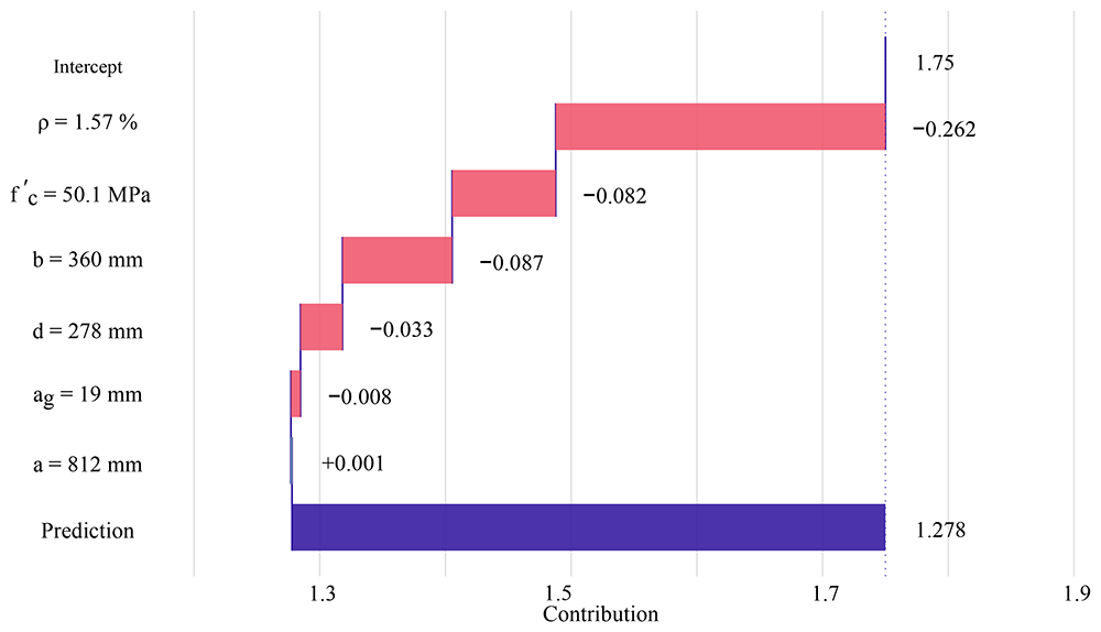
Figure A.9. BD profile for sample 1.

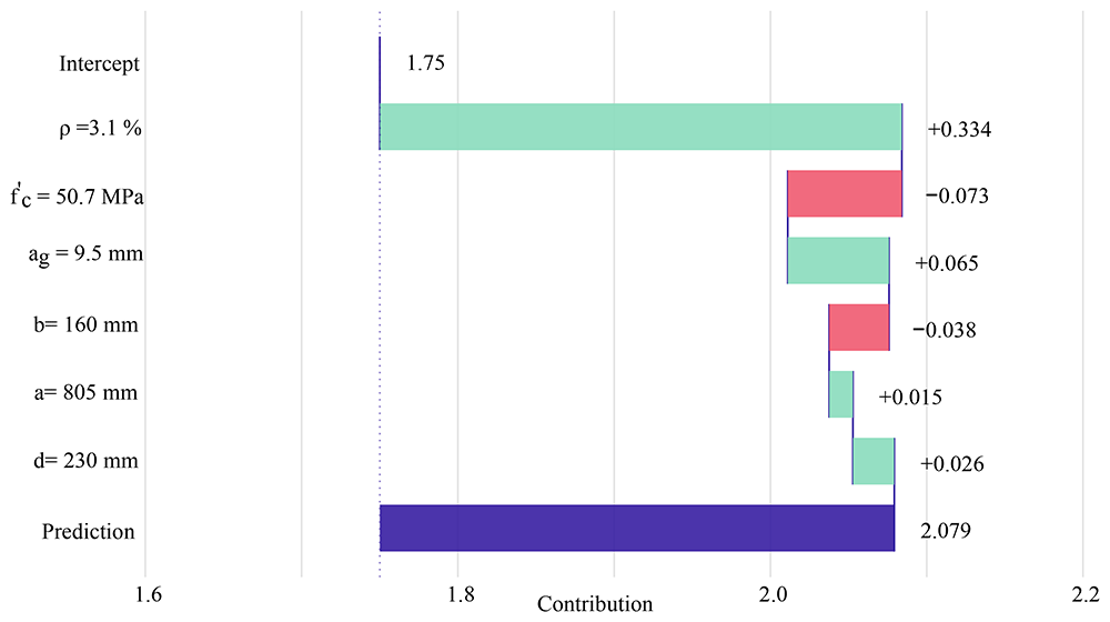
Figure A.10. BD profile for sample 2.

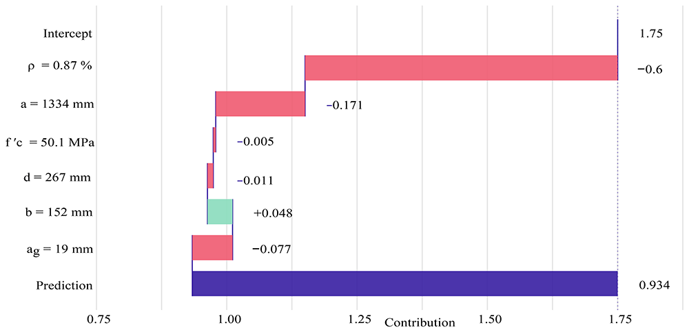
Figure A.11. BD profile for sample 3.

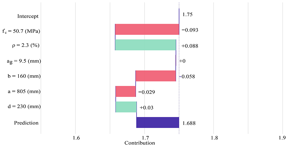
Figure A.12. BD profile for sample 4.

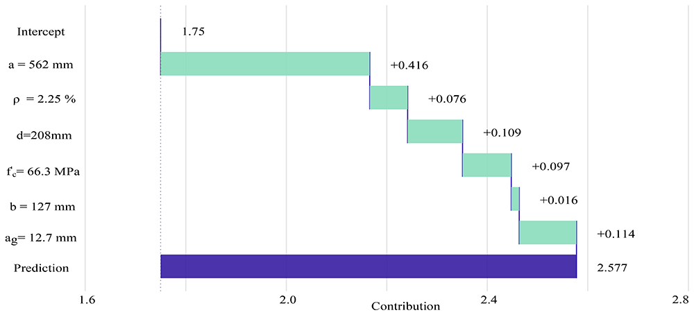
Figure A.13. BD profile for sample 5.

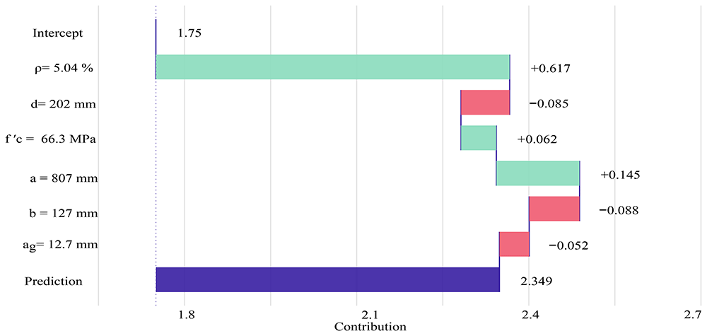
Figure A.14. BD profile for sample 6.

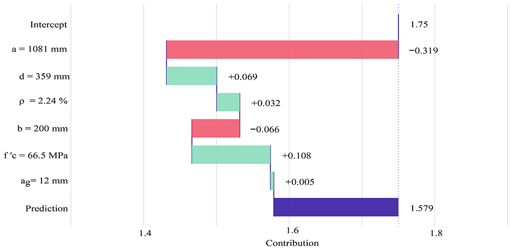
Figure A.15. BD profile for sample 7.

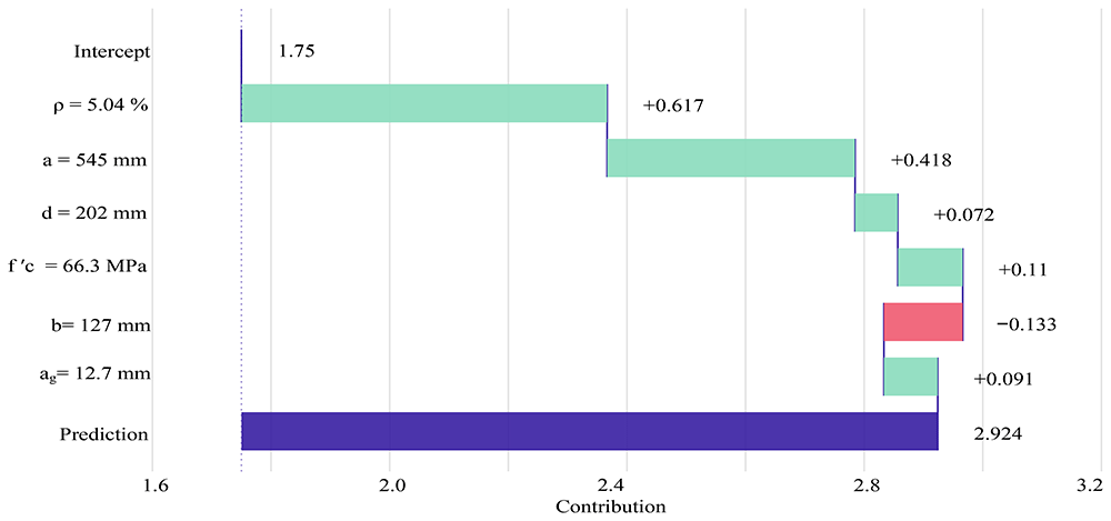
Figure A.16. BD profile for sample 8.

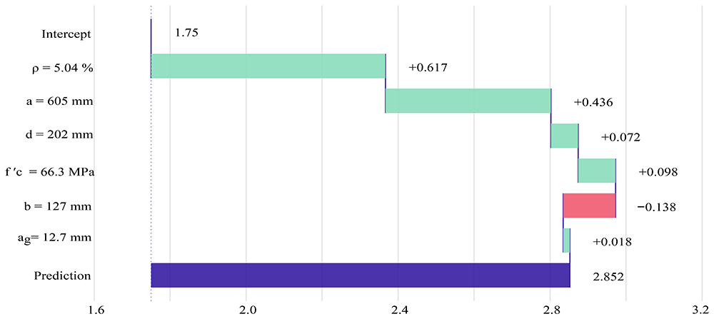
Figure A.17. BD profile for sample 9.

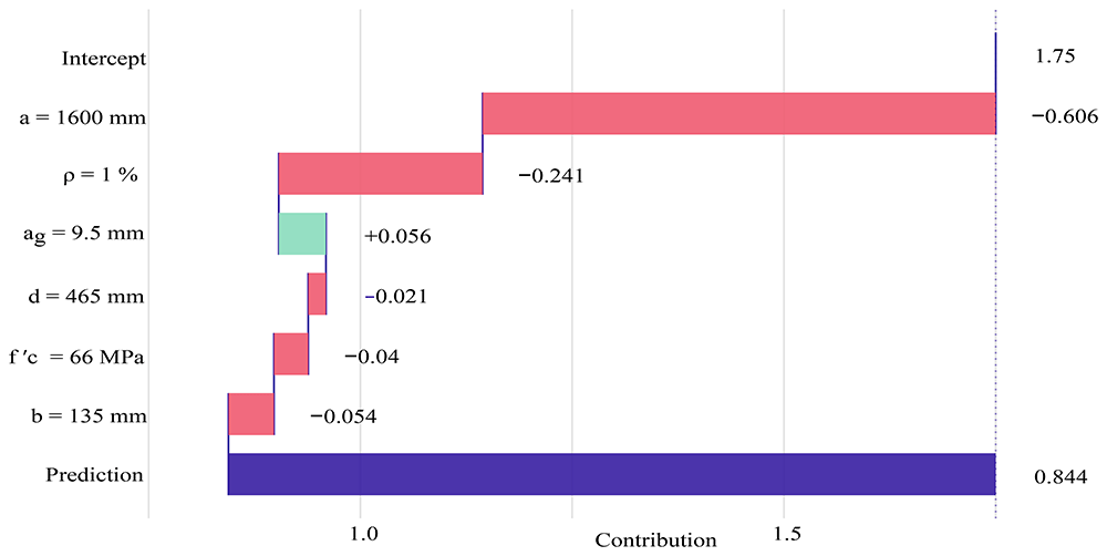
Figure A.18. BD profile for sample 10.

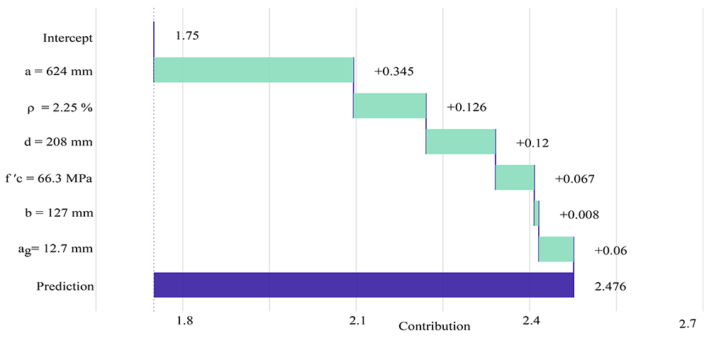
Figure A.19. BD profile for sample 11.

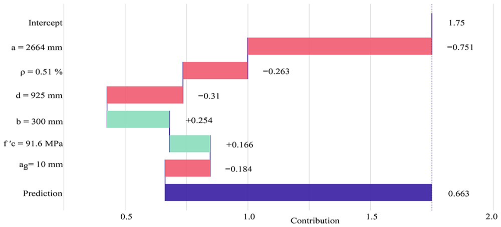
Figure A.20. BD profile for sample 12.

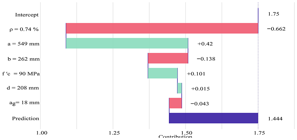
Figure A.21. BD profile for sample 13.

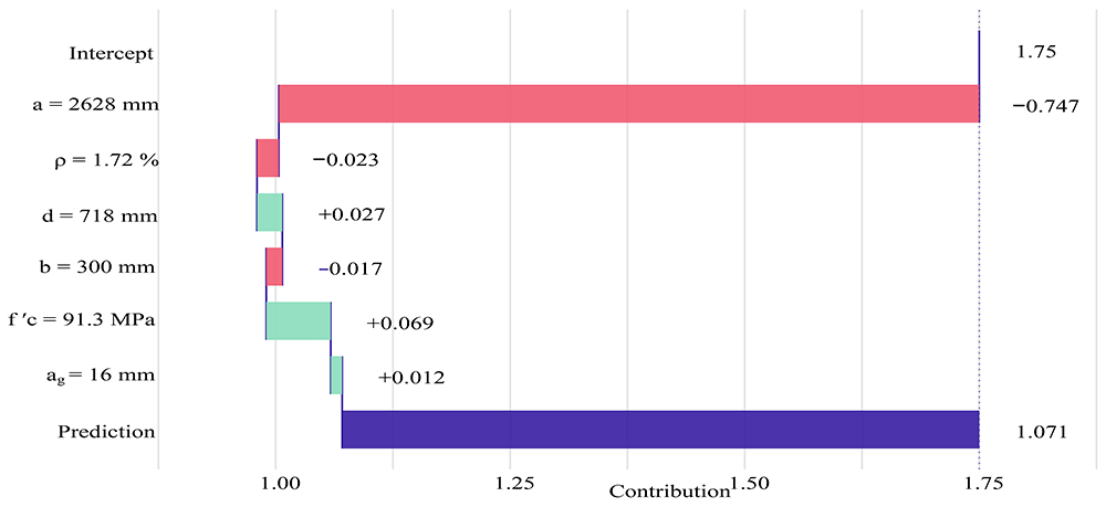
Figure A.22. BD profile for sample 14.

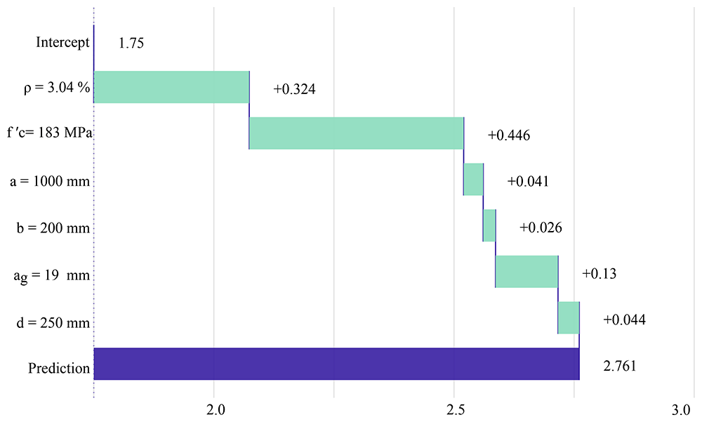
Figure A.23. BD profile for sample 15.

Appendix A.2. Results of SHAP techniques for all samples

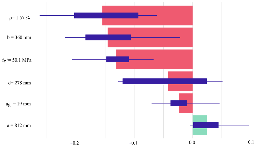
Figure A.24. SHAP profile with the average contributions for 25 random orderings using the sample 1.

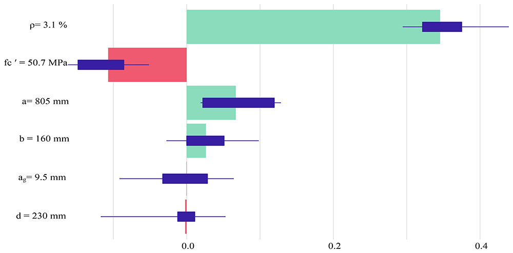
Figure A.25. SHAP profile with the average contributions for 25 random orderings using the sample 12.

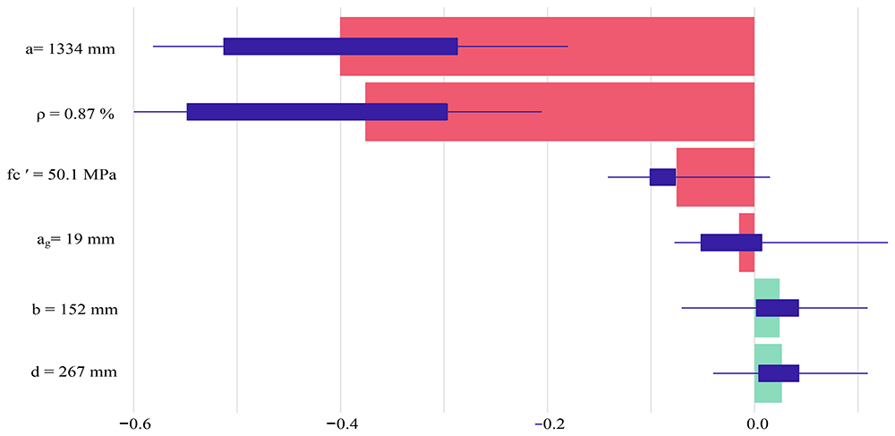
Figure A.26. SHAP profile with the average contributions for 25 random orderings using the sample 3.

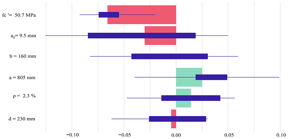
Figure A.27. SHAP profile with the average contributions for 25 random orderings using the sample 4.

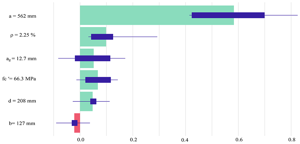
Figure A.28. SHAP profile with the average contributions for 25 random orderings using the sample 5.

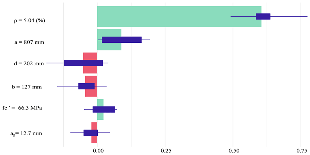
Figure A.29. SHAP profile with the average contributions for 25 random orderings using the sample 6.

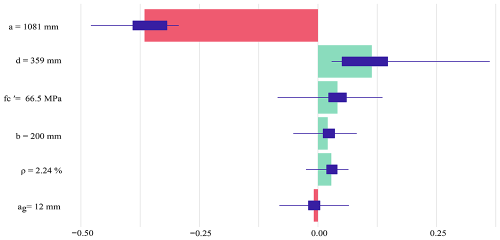
Figure A.30. SHAP profile with the average contributions for 25 random orderings using the sample 7.

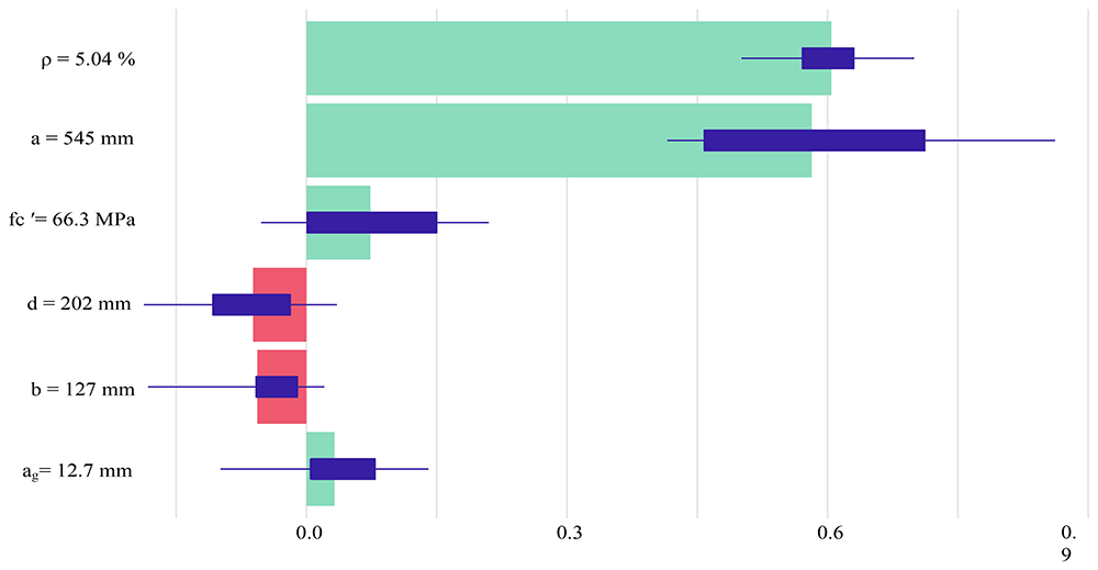
Figure A.31. SHAP profile with the average contributions for 25 random orderings using the sample 8.

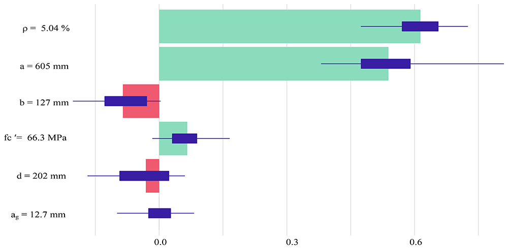
Figure A.32. SHAP profile with the average contributions for 25 random orderings using the sample 9.

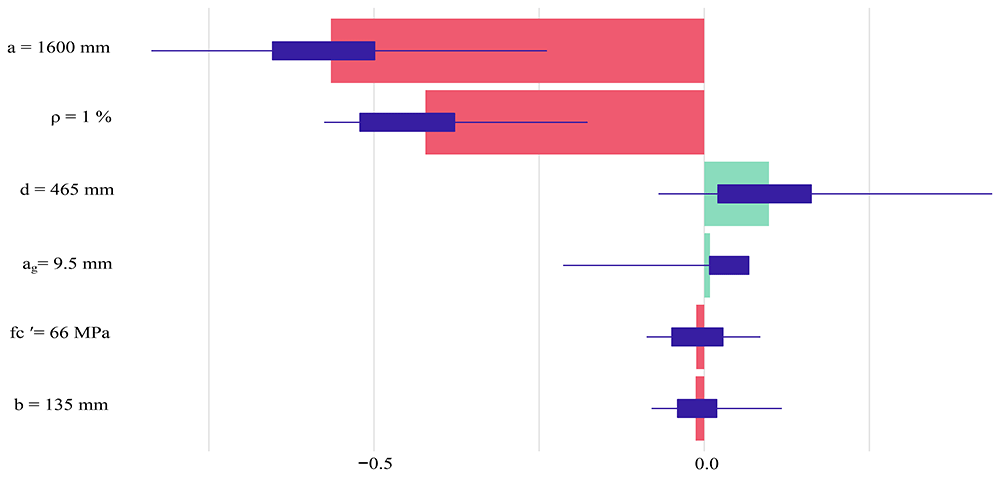
Figure A.33. SHAP profile with the average contributions for 25 random orderings using the sample 10.

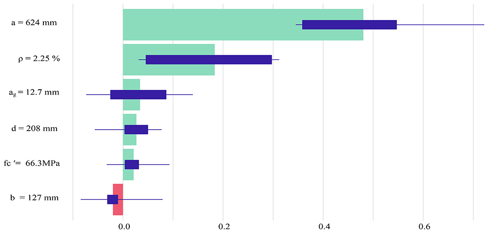
Figure A.34. SHAP profile with the average contributions for 25 random orderings using the sample 11.

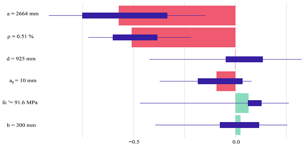
Figure A.35. SHAP profile with the average contributions for 25 random orderings using the sample 12.

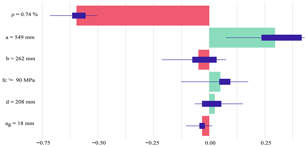
Figure A.36. SHAP profile with the average contributions for 25 random orderings using the sample 13.

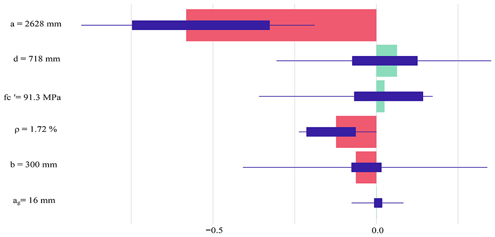
Figure A.37. SHAP profile with the average contributions for 25 random orderings using the sample 14.

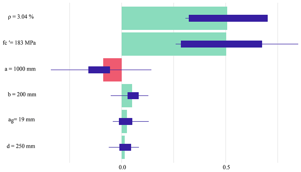
Figure A.38. SHAP profile with the average contributions for 25 random orderings using the sample 15.

Appendix B. Supplementary Material-B

Appendix B.1. Assessing explainer reliability via replication of results

In this section, each explainer technique was run nine times, and the SHAP and BD explanations for each data point were generated to ensure the results’ consistency. After gathering the results of the explainers, the average rank of each input parameter after nine runs is calculated (gray columns), then rounded and compared with the primary results (black columns). The results revealed that ρ, a, $f_{c}^{'}$ and a_g have consistent ranks, but there was variation in the ranks for d and b. Figure B.39 shows the fluctuation of SHAP and BD ranks for input parameters after nine running times.

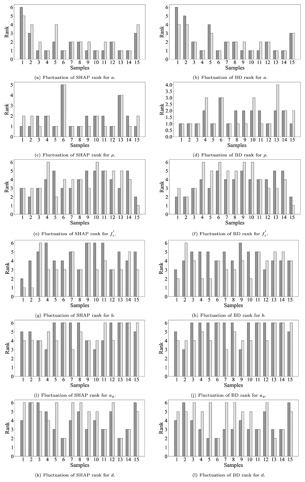
Figure B.39. Comparison of ranks of SHAP and BD techniques for various parameters after nine runs (black columns: primary results, gray columns: average of ranks).

Appendix B.2. External dataset testing of SHAP and BD explainers

In this section, we utilize various data points from different datasets^63,91,92 to assess the performance of SHAP and BD explainer techniques. The characteristics of these selected data points are presented in Table B.6.

Table B.6. Selected data points from other datasets for evaluating the explainer techniques.

Samples	d	a	a_g	$f_{c}^{'}$	ρ	b	v
1	211	485	13	64.3	0.53	127	0.493
2	211	844	13	64.3	0.53	127	0.145
3	265	450	19	70.9	2.65	100	0.742
4	207	475	13	64.3	3.26	127	0.943

Note: d, a, a_g, and b are in millimeters (mm). $f_{c}^{'}$ and v are in megapascals (MPa). ρ is expressed as a percentage (%).

The stacked ensemble 3 model was rerun five times, and the performances of SHAP and BD were evaluated in the same manner as in the previous section.

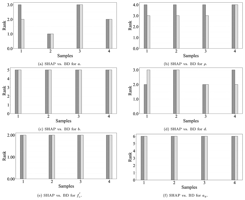
Figure B.40. Comparison of SHAP and BD results for various parameters after five runs (black columns: SHAP technique, gray columns: BD technique).

Figures B.40a,B.40b, B.40c, B.40d, B.40e and B.40f reveal that the parameters d, $f_{c}^{'}$ , a, and ρ have a greater impact on the prediction compared to b and a_g from other datasets which is inline with the previous findings in the current study.

Faculty Opinions recommended

References

1. American Concrete Institute: Report on High-Strength Concrete (aci prc-363-10), ACI Report PRC-363-10. American Concrete Institute, Farmington Hills, MI, 2010. Reference Source
2. Hamrat M, Boulekbache B, Chemrouk M, et al.: Shear Behaviour of RC beams without stirrups made of normal strength and High Strength Concretes. Advances in Structural Engineering. 2010; 13(1): 29–41. Publisher Full Text
3. Subramanian N: Evaluation and enhancing the punching shear resistance of flat slabs using HSC. The Indian Concrete Journal. 2005; 79(4): 31–37. Reference Source
4. Elsanadedy H, Abbas H, Al-Salloum Y, et al.: Shear strength prediction of HSC slender beams without web reinforcement. Materials and Structures. 2016; 49(9): 3749–3772. Publisher Full Text
5. Carrasquillo RL, Nilson AH, Slate FO: Properties of High Strength Concrete subjectto short-term loads. In: Journal Proceedings. 1981; 78(3): 171–178. Publisher Full Text
6. Kong PY: Shear strength of high performance concrete beams. Ph.D. thesis, Curtin University, 1996. Reference Source
7. Pendyala RS, Mendis P: Experimental study on shear strength of High-Strength Concrete beams. Structural Journal. 2000; 97(4): 564–571. Reference Source
8. Zsutty TC: Beam shear strength prediction by analysis of existing data. In: Journal Proceedings. 1968; 65(11): 943–951. Publisher Full Text
9. Kim JK, Park YD: Prediction of shear strength of reinforced concrete beams without web reinforcement. ACI Mater J. 1996; 93(3): 213–222. Publisher Full Text
10. Bažant ZP, Yu Q: Designing against size effect on shear strength of reinforced concrete beams without stirrups: Ii. Verification and calibration. J Struct Eng. 2005; 131(12): 1886–1897. Publisher Full Text
11. Al-Khafaji Z, Heddam S, Kim S, et al.: State-of-art: Artificial Intelligence models era in modeling beam shear strength. Knowledge-Based Engineering and Sciences. 2022; 3(3): 1–63. Reference Source
12. Jayasinghe T, Gunawardena T, Mendis P: Assessment of shear strength of reinforced concrete beams without shear reinforcement: a comparative study between codes of practice and artificial neural network. Case Studies in Construction Materials. 2022; 16: e01102. Publisher Full Text
13. Alyami M, Khan M, Fawad M, et al.: Predictive modeling for compressive strength of 3D printed fiber-reinforced concrete using machine learning algorithms. Case Studies in Construction Materials. 2024; 20: e02728. Publisher Full Text
14. Sandeep MS, Tiprak K, Kaewunruen S, et al.: Shear strength prediction of reinforced concrete beams using machine learning. In: Structures. Elsevier, 2023; 47: 1196–1211. Publisher Full Text
15. Cladera A, Mari A: Shear design procedure for reinforced normal and high-strength concrete beams using artificial neural networks. Part II: beams with stirrups. Engineering Structures. 2004; 26(7): 927–936. Publisher Full Text
16. Abdalla JA, Elsanosi A, Abdelwahab A: Modeling and simulation of shear resistance of R/C beams using artificial neural network. Journal of the Franklin Institute. 2007; 344(5): 741–756. Publisher Full Text
17. Jung S, Kim KS: Knowledge-based prediction of shear strength of concrete beams without shear reinforcement. Engineering Structures. 2008; 30(6): 1515–1525. Publisher Full Text
18. Mohammadhassani M, Nezamabadi-Pour H, Suhatril M, et al.: An evolutionary fuzzy modelling approach and comparison of different methods for shear strength prediction of High-Strength Concrete beams without stirrups. Smart Struct Syst. 2014; 14(5): 785–809. Reference Source
19. Sharafati A, Haghbin M, Aldlemy MS, et al.: Development of advanced computer aid model for shear strength of concrete slender beam prediction. Appl Sci. 2020; 10(11): 3811. Publisher Full Text
20. Ashour AF, Alvarez LF, Toropov VV: Empirical modelling of shear strength of RC deep beams by genetic programming. Computers & structures. 2003; 81(5): 331–338. Publisher Full Text
21. Gandomi AH, Alavi AH, Sahab MG: New formulation for compressive strength of CFRP confined concrete cylinders using linear genetic programming. Materials and Structures. 2010; 43(7): 963–983. Publisher Full Text
22. Gandomi AH, Yun GJ, Alavi AH: An evolutionary approach for modeling of shear strength of RC deep beams. Materials and structures. 2013; 46(12): 2109–2119. Publisher Full Text
23. Gandomi AH, Alavi AH, Kazemi S, et al.: Formulation of shear strength of slender RC beams using gene expression programming, part i: without shear reinforcement. Automation in Construction. 2014; 42: 112–121. Publisher Full Text
24. Yosri AM, Farouk AIB, Haruna SI, et al.: Sensitivity and robustness analysis of Adaptive Neuro-Fuzzy Inference System (ANFIS) for shear strength prediction of stud connectors in concrete. Case Studies in Construction Materials. 2023; 18: e02096. Publisher Full Text
25. Farzinpour A, Dehcheshmeh EM, Broujerdian V, et al.: Efficient boosting-based algorithms for shear strength prediction of squat RC walls. Case Studies in Construction Materials. 2023; 18: e01928. Publisher Full Text
26. Pal M, Deswal S: Support vector regression based shear strength modelling of deep beams. Computers & Structures. 2011; 89(13–14): 1430–1439. Publisher Full Text
27. Yaseen ZM: Machine learning models development for shear strength prediction of reinforced concrete beam: a comparative study. Sci Rep. 2023; 13(1): 1723. Publisher Full Text
28. Yaseen ZM, Deo RC, Hilal A, et al.: Predicting compressive strength of lightweight foamed concrete using extreme learning machine model. Advances in Engineering Software. 2018; 115: 112–125. Publisher Full Text
29. Al-Abdaly NM, Hussein MJ, Imran H, et al.: Shear strength prediction of steel-fiber-reinforced concrete beams using the M5P model. Fibers. 2023; 11(5): 37. Publisher Full Text
30. Shatnawi A, Alkassar HM, Al-Abdaly NM, et al.: Shear strength prediction of slender steel fiber reinforced concrete beams using a gradient boosting regression tree method. Buildings. 2022; 12(5): 550. Publisher Full Text
31. Olalusi OB, Awoyera PO: Shear capacity prediction of slender Reinforced Concrete structures with steel fibers using machine learning. Engineering Structures. 2021; 227: 111470. Publisher Full Text
32. Zednik C: Solving the black box problem: a normative framework for explainable Artificial Intelligence. Philosophy & Technology. 2021; 34(2): 265–288. Publisher Full Text
33. Yu R, Alì GS: What’s inside the black box? AI challenges for lawyers and researchers. Legal Information Management. 2019; 19(1): 2–13. Publisher Full Text
34. Mangalathu S, Hwang SH, Jeon JS: Failure mode and effects analysis of RC members based on machine-learning-based SHapley Additive exPlanations (SHAP) approach. Engineering Structures. 2020; 219: 110927. Publisher Full Text
35. Mangalathu S, Shin H, Choi E, et al.: Explainable machine learning models for punching shear strength estimation of flat slabs without transverse reinforcement. J Build Eng. 2021; 39: 102300. Publisher Full Text
36. Le Nguyen K, Trinh HT, Nguyen TT, et al.: Comparative study on the performance of different machine learning techniques to predict the shear strength of RC deep beams: model selection and industry implications. Expert Systems with Applications. 2023; 230: 120649. Publisher Full Text
37. Nguyen KL, Trinh HT, Pham TM: Prediction of punching shear strength in flat slabs: ensemble learning models and practical implementation. Neural Computing and Applications. 2024; 36: 4207–4228. Publisher Full Text
38. Liu T, Cakiroglu C, Islam K, et al.: Explainable machine learning model for predicting punching shear strength of FRC flat slabs. Engineering Structures. 2024; 301: 117276. Publisher Full Text
39. Nguyen TA, Ly HB, Tran VQ: Predicting shear strength of slender beams without reinforcement using hybrid gradient boosting trees and optimization algorithms. Frontiers of Structural and Civil Engineering. 2022; 16(10): 1267–1286. Publisher Full Text
40. Arrieta AB, Díaz-Rodríguez N, Del Ser J, et al.: Explainable Artificial Intelligence (XAI): concepts, taxonomies, opportunities and challenges toward responsible AI. Information Fusion. 2020; 58: 82–115. Publisher Full Text
41. Tiwari A, Gupta AK, Gupta T: A robust approach to shear strength prediction of reinforced concrete deep beams using ensemble learning with SHAP interpretability. Soft Comput. 2024; 28(7): 6343–6365. Publisher Full Text
42. Feng DC, Wang WJ, Mangalathu S, et al.: Interpretable XGBoost-SHAP machine-learning model for shear strength prediction of squat RC walls. J Struct Eng. 2021; 147(11): 04021173. Publisher Full Text
43. Cheng C, Taffese WZ, Hu T: Accurate prediction of punching shear strength of steel fiber-reinforced concrete slabs: a machine learning approach with data augmentation and explainability. Buildings. 2024; 14(5): 1223. Publisher Full Text
44. Christoph M: Interpretable machine learning: a guide for making black box models explainable. Leanpub. 2020. Reference Source
45. Slack D, Hilgard S, Jia E, et al.: Fooling LIME and SHAP: adversarial attacks on post hoc explanation methods. In: Proceedings of the AAAI/ACM Conference on AI, Ethics, and Society. 2020; 180–186. Publisher Full Text
46. Laberge G, Aïvodji U, Hara S, et al.: Fool shap with stealthily biased sampling. arXiv preprint arXiv: 2205.15419. Publisher Full Text
47. Yuan J, Dasgupta A: Fooling SHAP with output shuffling attacks. arXiv preprint arXiv: 2408.06509. Publisher Full Text
48. Marques-Silva J, Huang X: Explainability is not a game. Communications of the ACM. 2024; 67(7): 66–75. Publisher Full Text
49. Shah A, Ahmad S: An experimental investigation into shear capacity of High Strength Concrete beams. Asian Journal of Civil Engineering (building and housing). 2007; 549–562. Reference Source
50. Collins MP, Kuchma D: How safe are our large, lightly reinforced concrete beams, slabs, and footings? Struct J. 1999; 96(4): 482–490. Publisher Full Text
51. Al-Shaleh K, Rahal KN: Shear behavior of K850 reinforced concrete beams with low transverse reinforcement. Kuwait J Sci Eng. 2007; 34(2B): 35–54. Reference Source
52. Sagaseta J, Vollum RL: Non-linear finite element analysis of shear critical high strength concrete beams. Architecture Civil Engineering Environment-ACEE. 2009; 2(4): 95–106. Reference Source
53. Eisa ASA: Shear strength of high strength concrete beams. Master’s Thesis, Zagazig University, Zagazig, Egypt.
54. Bozorg-Haddad O, Soleimani S, Loáiciga HA: Modeling water-quality parameters using genetic algorithm-least squares support vector regression and genetic programming. J Environ Eng. 2017; 143(7): 04017021. Publisher Full Text
55. Joint ACI-ASCE Committee 326, Behavior and strength of reinforced concrete beams, Aci publication sp-12, American Concrete Institute (ACI) and American Society of Civil Engineers (ASCE), Detroit, MI (1962).
56. Joint ACI-ASCE Committee 426, Shear and torsion, Aci publication sp-42, American Concrete Institute (ACI) and American Society of Civil Engineers (ASCE), Detroit, MI (1973).
57. MacGregor JG, Hanson J: Strength and behavior of reinforced concrete under load. ACI Journal. 1969; 66(3): 180–191.
58. Ruiz MF, Muttoni A, Sagaseta J: Shear strength of concrete members without transverse reinforcement: a mechanical approach to consistently account for size and strain effects. Eng Struct. 2015; 99: 360–372. Publisher Full Text
59. Muttoni A, Fernández Ruiz M: Shear strength of members without transverse reinforcement as function of critical shear crack width. ACI Struct J. 2008; 105(2): 163–172. Publisher Full Text
60. Campana S, Fernández Ruiz M, Anastasi A, et al.: Analysis of shear-transfer actions on one-way RC members based on measured cracking pattern and failure kinematics. Magazine of Concrete Research. 2013; 65(6): 386–404. Publisher Full Text
61. American Concrete Institute, Farmington Hills, MI: Building code requirements for structural concrete (ACI 318-19) and commentary (ACI 318R-19). 2019th Edition, 2019. Reference Source
62. C. Européen: Eurocode 2: design of concrete structures—Part 1-1: general rules and rules for buildings. London: British Standard Institution.
63. Ahmad SH, Lue D: Flexure-shear interaction of reinforced high strength concrete beams. Struct J. 1987; 84(4): 330–341. Publisher Full Text
64. Yang KH, Chung HS, Ashour A: Influence of section depth on the structural behaviour of reinforced concrete continuous deep beams. Magazine of Concrete Research. 2007; 59(8): 575–586. Publisher Full Text
65. C.S. Eurocodes: Eurocode 2: design of concrete structures — Part 1-1: general rules and rules for buildings. Standard FprEN 1992-1-1: 2022, European Committee for Standardization, Brussels, 2022.
66. Taylor HPJ: Investigation of the forces carried across cracks in reinforced concrete beams in shear by interlock of aggregate. Tech. rep., Transport and Road Research Laboratory (TRRL), 1970. Reference Source
67. Gebreyouhannes E, Maekawa K: Numerical simulation on shear capacity and post-peak ductility of reinforced High-Strength Concrete coupled with autogenous shrinkage. Journal of Advanced Concrete Technology. 2011; 9(1): 73–88. Publisher Full Text
68. Sagaseta J, Vollum R: Influence of aggregate fracture on shear transfer through cracks in reinforced concrete. Magazine of Concrete Research. 2011; 63(2): 119–137. Publisher Full Text
69. Elzanaty AH, Nilson AH, Slate FO: Shear capacity of reinforced concrete beams using high-strength concrete. In: Journal Proceedings. 1986; 83(2): 290–296. Publisher Full Text
70. Mphonde AG, Frantz GC: Shear tests of high- and low-strength concrete beams without stirrups. In: Journal Proceedings. 1984; 81(4): 350–357. Publisher Full Text
71. Mphonde A: Aggregate interlock in high strength reinforced concrete beams. Proceedings of the Institution of Civil Engineers. 1988; 85(3): 397–413. Publisher Full Text
72. Cladera A, Marí A: Shear design procedure for reinforced normal and High-Strength Concrete beams using artificial neural networks. Part I: beams without stirrups. Eng Struct. 2004; 26(7): 917–926. Publisher Full Text
73. Kim JK, Park YD: Shear strength of reinforced high strength concrete beams without web reinforcement. Magazine of concrete research. 1994; 46(166): 7–16. Publisher Full Text
74. Kim KS: Shear behavior of reinforced concrete beams and prestressed concrete beams. Ph.D. thesis, University of Illinois at Urbana-Champaign, 2004. Reference Source
75. Ribeiro MT, Singh S, Guestrin C: "Why Should I Trust You?" Explaining the predictions of any classifier. In: Proceedings of the 22nd ACM SIGKDD international conference on knowledge discovery and data mining. 2016; 1135–1144. Publisher Full Text
76. Ghai B, Liao QV, Zhang Y, et al.: Explainable Active Learning (XAL): toward AI explanations as interfaces for machine teachers. Proceedings of the ACM on Human-Computer Interaction 4 (CSCW3). 2021; 1–28. Publisher Full Text
77. Bodria F, Giannotti F, Guidotti R, et al.: Benchmarking and survey of explanation methods for black box models. Data Min Knowl Discov. 2023; 37(5): 1719–1778. Publisher Full Text
78. Linardatos P, Papastefanopoulos V, Kotsiantis S: Explainable AI: a review of machine learning interpretability methods. Entropy (Basel). 2020; 23(1): 18. PubMed Abstract | Publisher Full Text | Free Full Text
79. Staniak M, Biecek P: Explanations of model predictions with live and breakDown packages. arXiv preprint arXiv: 1804.01955. Publisher Full Text
80. Lundberg SM, Lee SI: A unified approach to interpreting model predictions. Advances in neural information processing systems. 30.
81. Shapley LS: Contributions to the theory of games. Chapter A value for n-person games. Ann Math Stud.
82. Parsa AB, Movahedi A, Taghipour H, et al.: Toward safer highways, application of XGBoost and SHAP for real-time accident detection and feature analysis. Accid Anal Prev. 2020; 136: 105405. PubMed Abstract | Publisher Full Text
83. Qi Y: Random Forest for bioinformatics. Ensemble machine learning: Methods and applications. 2012; 307–323. Publisher Full Text
84. Bahad P, Saxena P: Study of adaboost and gradient boosting algorithms for predictive analytics. In: International Conference on Intelligent Computing and Smart Communication 2019: Proceedings of ICSC 2019, Springer, 2020; 235–244. Publisher Full Text
85. Haghbin M, Sharafati A, Dixon B, et al.: Application of soft computing models for simulating nitrate contamination in groundwater: comprehensive review, assessment and future opportunities. Arch Comput Methods Eng. 2021; 28(5): 3569–3591. Publisher Full Text
86. Biecek P: Dalex: explainers for complex predictive models in R. J Mach Learn Res. 2018; 19(84): 1–5. Reference Source
87. Maksymiuk S, Gosiewska A, Biecek P: Landscape of R packages for eXplainable Artificial Intelligence. arXiv preprint arXiv: 2009.13248. Publisher Full Text
88. Aiello S, Eckstrand E, Fu A, et al.: Machine learning with R and H2O. H2O booklet 550. Reference Source
89. Qiu D, Tamhane AC: A comparative study of the K-means algorithm and the normal mixture model for clustering: univariate case. J Stat Plan Inference. 2007; 137(11): 3722–3740. Publisher Full Text
90. Koza JR, Rice JP: Automatic programming of robots using genetic programming. In: AAAI. Citeseer, 1992; 92. : 194–207. Reference Source
91. Xie Y, Ahmad SH, Yu T, et al.: Shear ductility of reinforced concrete beams of normal and high-strength concrete. Struct J. 1994; 91(2): 140–149. Publisher Full Text
92. Yuichi M, Norihiko K, Yuichi U, et al.: Shear capacity of reinforced high strength concrete beams without shear reinforcement. Transactions of the Japan Concrete Institute. 1996; 17: 319–326. Reference Source
93. Meurer A: gplearn: genetic programming in python. accessed: 2024–11–11. Reference Source
94. High-Level Expert Group on AI European Commission: Ethics guidelines for trustworthy AI. 2019. Reference Source

Comments

Publication information

Section

Research Article

Published

April 25, 2025

DOI

https://doi.org/10.12688/openreseurope.20195.1

Versions

April 25, 2025 (Published Manuscript Under Review 1.0)

Included in

Funding data

European Commission

Grant ID(s): 101092052

Metrics

Views

Downloads

Citations

See full metrics

Keywords

Shear strength, High-Strength Concrete, Explainable Artificial Intelligence.

Comments

Masoud Haghbin

Department of Structural Mechanics and Hydraulic Engineering, University of Granada, Granada, Andalusia, 18071, Spain

Andalusian Research Institute in Data Science and Computational Intelligence (DaSCI), University of Granada, Granada, Andalusia, 18071, Spain

Roles

Co-Author, Conceptualization, Methodology, Writing – Original Draft Preparation

0000-0002-2042-6645

m.haghbin89@gmail.com

María L. Jalón

Department of Structural Mechanics and Hydraulic Engineering, University of Granada, Granada, Andalusia, 18071, Spain

Roles

Co-Author, Supervision, Validation, Writing – Original Draft Preparation, Writing – Review & Editing

mljalon@go.ugr.es

Natalia Díaz-Rodríguez

Andalusian Research Institute in Data Science and Computational Intelligence (DaSCI), University of Granada, Granada, Andalusia, 18071, Spain

Department of Computer Science and Artificial Intelligence, University of Granada (UGR), CITIC, University of Granada, Granada, Andalusia, 18071, Spain

Roles

Co-Author, Validation, Writing – Review & Editing

nataliadiaz@ugr.es

Juan Chiachío

Department of Structural Mechanics and Hydraulic Engineering, University of Granada, Granada, Andalusia, 18071, Spain

Andalusian Research Institute in Data Science and Computational Intelligence (DaSCI), University of Granada, Granada, Andalusia, 18071, Spain

Roles

Corresponding Author, Co-Author, Methodology, Supervision, Validation, Writing – Review & Editing

jchiachio@ugr.es

Downloads over the last 12 months:

Cited by

via Crossref

View citing articles

[1] 1. American Concrete Institute: Report on High-Strength Concrete (aci prc-363-10), ACI Report PRC-363-10. American Concrete Institute, Farmington Hills, MI, 2010. Reference Source

[2] 2. Hamrat M, Boulekbache B, Chemrouk M, et al.: Shear Behaviour of RC beams without stirrups made of normal strength and High Strength Concretes. Advances in Structural Engineering. 2010; 13(1): 29–41. Publisher Full Text

[3] 3. Subramanian N: Evaluation and enhancing the punching shear resistance of flat slabs using HSC. The Indian Concrete Journal. 2005; 79(4): 31–37. Reference Source

[4] 4. Elsanadedy H, Abbas H, Al-Salloum Y, et al.: Shear strength prediction of HSC slender beams without web reinforcement. Materials and Structures. 2016; 49(9): 3749–3772. Publisher Full Text

[5] 5. Carrasquillo RL, Nilson AH, Slate FO: Properties of High Strength Concrete subjectto short-term loads. In: Journal Proceedings. 1981; 78(3): 171–178. Publisher Full Text

[6] 6. Kong PY: Shear strength of high performance concrete beams. Ph.D. thesis, Curtin University, 1996. Reference Source

[7] 7. Pendyala RS, Mendis P: Experimental study on shear strength of High-Strength Concrete beams. Structural Journal. 2000; 97(4): 564–571. Reference Source

[8] 8. Zsutty TC: Beam shear strength prediction by analysis of existing data. In: Journal Proceedings. 1968; 65(11): 943–951. Publisher Full Text

[9] 9. Kim JK, Park YD: Prediction of shear strength of reinforced concrete beams without web reinforcement. ACI Mater J. 1996; 93(3): 213–222. Publisher Full Text

[10] 10. Bažant ZP, Yu Q: Designing against size effect on shear strength of reinforced concrete beams without stirrups: Ii. Verification and calibration. J Struct Eng. 2005; 131(12): 1886–1897. Publisher Full Text

[11] 11. Al-Khafaji Z, Heddam S, Kim S, et al.: State-of-art: Artificial Intelligence models era in modeling beam shear strength. Knowledge-Based Engineering and Sciences. 2022; 3(3): 1–63. Reference Source

[12] 12. Jayasinghe T, Gunawardena T, Mendis P: Assessment of shear strength of reinforced concrete beams without shear reinforcement: a comparative study between codes of practice and artificial neural network. Case Studies in Construction Materials. 2022; 16: e01102. Publisher Full Text

[13] 13. Alyami M, Khan M, Fawad M, et al.: Predictive modeling for compressive strength of 3D printed fiber-reinforced concrete using machine learning algorithms. Case Studies in Construction Materials. 2024; 20: e02728. Publisher Full Text

[14] 14. Sandeep MS, Tiprak K, Kaewunruen S, et al.: Shear strength prediction of reinforced concrete beams using machine learning. In: Structures. Elsevier, 2023; 47: 1196–1211. Publisher Full Text

[15] 15. Cladera A, Mari A: Shear design procedure for reinforced normal and high-strength concrete beams using artificial neural networks. Part II: beams with stirrups. Engineering Structures. 2004; 26(7): 927–936. Publisher Full Text

[16] 16. Abdalla JA, Elsanosi A, Abdelwahab A: Modeling and simulation of shear resistance of R/C beams using artificial neural network. Journal of the Franklin Institute. 2007; 344(5): 741–756. Publisher Full Text

[17] 17. Jung S, Kim KS: Knowledge-based prediction of shear strength of concrete beams without shear reinforcement. Engineering Structures. 2008; 30(6): 1515–1525. Publisher Full Text

[18] 18. Mohammadhassani M, Nezamabadi-Pour H, Suhatril M, et al.: An evolutionary fuzzy modelling approach and comparison of different methods for shear strength prediction of High-Strength Concrete beams without stirrups. Smart Struct Syst. 2014; 14(5): 785–809. Reference Source

[19] 19. Sharafati A, Haghbin M, Aldlemy MS, et al.: Development of advanced computer aid model for shear strength of concrete slender beam prediction. Appl Sci. 2020; 10(11): 3811. Publisher Full Text

[20] 20. Ashour AF, Alvarez LF, Toropov VV: Empirical modelling of shear strength of RC deep beams by genetic programming. Computers & structures. 2003; 81(5): 331–338. Publisher Full Text

[21] 21. Gandomi AH, Alavi AH, Sahab MG: New formulation for compressive strength of CFRP confined concrete cylinders using linear genetic programming. Materials and Structures. 2010; 43(7): 963–983. Publisher Full Text

[22] 22. Gandomi AH, Yun GJ, Alavi AH: An evolutionary approach for modeling of shear strength of RC deep beams. Materials and structures. 2013; 46(12): 2109–2119. Publisher Full Text

[23] 23. Gandomi AH, Alavi AH, Kazemi S, et al.: Formulation of shear strength of slender RC beams using gene expression programming, part i: without shear reinforcement. Automation in Construction. 2014; 42: 112–121. Publisher Full Text

[24] 24. Yosri AM, Farouk AIB, Haruna SI, et al.: Sensitivity and robustness analysis of Adaptive Neuro-Fuzzy Inference System (ANFIS) for shear strength prediction of stud connectors in concrete. Case Studies in Construction Materials. 2023; 18: e02096. Publisher Full Text

[25] 25. Farzinpour A, Dehcheshmeh EM, Broujerdian V, et al.: Efficient boosting-based algorithms for shear strength prediction of squat RC walls. Case Studies in Construction Materials. 2023; 18: e01928. Publisher Full Text

[26] 26. Pal M, Deswal S: Support vector regression based shear strength modelling of deep beams. Computers & Structures. 2011; 89(13–14): 1430–1439. Publisher Full Text

[27] 27. Yaseen ZM: Machine learning models development for shear strength prediction of reinforced concrete beam: a comparative study. Sci Rep. 2023; 13(1): 1723. Publisher Full Text

[28] 28. Yaseen ZM, Deo RC, Hilal A, et al.: Predicting compressive strength of lightweight foamed concrete using extreme learning machine model. Advances in Engineering Software. 2018; 115: 112–125. Publisher Full Text

[29] 29. Al-Abdaly NM, Hussein MJ, Imran H, et al.: Shear strength prediction of steel-fiber-reinforced concrete beams using the M5P model. Fibers. 2023; 11(5): 37. Publisher Full Text

[30] 30. Shatnawi A, Alkassar HM, Al-Abdaly NM, et al.: Shear strength prediction of slender steel fiber reinforced concrete beams using a gradient boosting regression tree method. Buildings. 2022; 12(5): 550. Publisher Full Text

[31] 31. Olalusi OB, Awoyera PO: Shear capacity prediction of slender Reinforced Concrete structures with steel fibers using machine learning. Engineering Structures. 2021; 227: 111470. Publisher Full Text

[32] 32. Zednik C: Solving the black box problem: a normative framework for explainable Artificial Intelligence. Philosophy & Technology. 2021; 34(2): 265–288. Publisher Full Text

[33] 33. Yu R, Alì GS: What’s inside the black box? AI challenges for lawyers and researchers. Legal Information Management. 2019; 19(1): 2–13. Publisher Full Text

[34] 34. Mangalathu S, Hwang SH, Jeon JS: Failure mode and effects analysis of RC members based on machine-learning-based SHapley Additive exPlanations (SHAP) approach. Engineering Structures. 2020; 219: 110927. Publisher Full Text

[35] 35. Mangalathu S, Shin H, Choi E, et al.: Explainable machine learning models for punching shear strength estimation of flat slabs without transverse reinforcement. J Build Eng. 2021; 39: 102300. Publisher Full Text

[36] 36. Le Nguyen K, Trinh HT, Nguyen TT, et al.: Comparative study on the performance of different machine learning techniques to predict the shear strength of RC deep beams: model selection and industry implications. Expert Systems with Applications. 2023; 230: 120649. Publisher Full Text

[37] 37. Nguyen KL, Trinh HT, Pham TM: Prediction of punching shear strength in flat slabs: ensemble learning models and practical implementation. Neural Computing and Applications. 2024; 36: 4207–4228. Publisher Full Text

[38] 38. Liu T, Cakiroglu C, Islam K, et al.: Explainable machine learning model for predicting punching shear strength of FRC flat slabs. Engineering Structures. 2024; 301: 117276. Publisher Full Text

[39] 39. Nguyen TA, Ly HB, Tran VQ: Predicting shear strength of slender beams without reinforcement using hybrid gradient boosting trees and optimization algorithms. Frontiers of Structural and Civil Engineering. 2022; 16(10): 1267–1286. Publisher Full Text

[40] 40. Arrieta AB, Díaz-Rodríguez N, Del Ser J, et al.: Explainable Artificial Intelligence (XAI): concepts, taxonomies, opportunities and challenges toward responsible AI. Information Fusion. 2020; 58: 82–115. Publisher Full Text

[41] 41. Tiwari A, Gupta AK, Gupta T: A robust approach to shear strength prediction of reinforced concrete deep beams using ensemble learning with SHAP interpretability. Soft Comput. 2024; 28(7): 6343–6365. Publisher Full Text

[42] 42. Feng DC, Wang WJ, Mangalathu S, et al.: Interpretable XGBoost-SHAP machine-learning model for shear strength prediction of squat RC walls. J Struct Eng. 2021; 147(11): 04021173. Publisher Full Text

[43] 43. Cheng C, Taffese WZ, Hu T: Accurate prediction of punching shear strength of steel fiber-reinforced concrete slabs: a machine learning approach with data augmentation and explainability. Buildings. 2024; 14(5): 1223. Publisher Full Text

[44] 44. Christoph M: Interpretable machine learning: a guide for making black box models explainable. Leanpub. 2020. Reference Source

[45] 45. Slack D, Hilgard S, Jia E, et al.: Fooling LIME and SHAP: adversarial attacks on post hoc explanation methods. In: Proceedings of the AAAI/ACM Conference on AI, Ethics, and Society. 2020; 180–186. Publisher Full Text

[46] 46. Laberge G, Aïvodji U, Hara S, et al.: Fool shap with stealthily biased sampling. arXiv preprint arXiv: 2205.15419. Publisher Full Text

[47] 47. Yuan J, Dasgupta A: Fooling SHAP with output shuffling attacks. arXiv preprint arXiv: 2408.06509. Publisher Full Text

[48] 48. Marques-Silva J, Huang X: Explainability is not a game. Communications of the ACM. 2024; 67(7): 66–75. Publisher Full Text

[49] 49. Shah A, Ahmad S: An experimental investigation into shear capacity of High Strength Concrete beams. Asian Journal of Civil Engineering (building and housing). 2007; 549–562. Reference Source

[50] 50. Collins MP, Kuchma D: How safe are our large, lightly reinforced concrete beams, slabs, and footings? Struct J. 1999; 96(4): 482–490. Publisher Full Text

[51] 51. Al-Shaleh K, Rahal KN: Shear behavior of K850 reinforced concrete beams with low transverse reinforcement. Kuwait J Sci Eng. 2007; 34(2B): 35–54. Reference Source

[52] 52. Sagaseta J, Vollum RL: Non-linear finite element analysis of shear critical high strength concrete beams. Architecture Civil Engineering Environment-ACEE. 2009; 2(4): 95–106. Reference Source

[53] 53. Eisa ASA: Shear strength of high strength concrete beams. Master’s Thesis, Zagazig University, Zagazig, Egypt.

[54] 54. Bozorg-Haddad O, Soleimani S, Loáiciga HA: Modeling water-quality parameters using genetic algorithm-least squares support vector regression and genetic programming. J Environ Eng. 2017; 143(7): 04017021. Publisher Full Text

[55] 55. Joint ACI-ASCE Committee 326, Behavior and strength of reinforced concrete beams, Aci publication sp-12, American Concrete Institute (ACI) and American Society of Civil Engineers (ASCE), Detroit, MI (1962).

[56] 56. Joint ACI-ASCE Committee 426, Shear and torsion, Aci publication sp-42, American Concrete Institute (ACI) and American Society of Civil Engineers (ASCE), Detroit, MI (1973).

[57] 57. MacGregor JG, Hanson J: Strength and behavior of reinforced concrete under load. ACI Journal. 1969; 66(3): 180–191.

[58] 58. Ruiz MF, Muttoni A, Sagaseta J: Shear strength of concrete members without transverse reinforcement: a mechanical approach to consistently account for size and strain effects. Eng Struct. 2015; 99: 360–372. Publisher Full Text

[59] 59. Muttoni A, Fernández Ruiz M: Shear strength of members without transverse reinforcement as function of critical shear crack width. ACI Struct J. 2008; 105(2): 163–172. Publisher Full Text

[60] 60. Campana S, Fernández Ruiz M, Anastasi A, et al.: Analysis of shear-transfer actions on one-way RC members based on measured cracking pattern and failure kinematics. Magazine of Concrete Research. 2013; 65(6): 386–404. Publisher Full Text

[61] 61. American Concrete Institute, Farmington Hills, MI: Building code requirements for structural concrete (ACI 318-19) and commentary (ACI 318R-19). 2019th Edition, 2019. Reference Source

[62] 62. C. Européen: Eurocode 2: design of concrete structures—Part 1-1: general rules and rules for buildings. London: British Standard Institution.

[63] 63. Ahmad SH, Lue D: Flexure-shear interaction of reinforced high strength concrete beams. Struct J. 1987; 84(4): 330–341. Publisher Full Text

[64] 64. Yang KH, Chung HS, Ashour A: Influence of section depth on the structural behaviour of reinforced concrete continuous deep beams. Magazine of Concrete Research. 2007; 59(8): 575–586. Publisher Full Text

[65] 65. C.S. Eurocodes: Eurocode 2: design of concrete structures — Part 1-1: general rules and rules for buildings. Standard FprEN 1992-1-1: 2022, European Committee for Standardization, Brussels, 2022.

[66] 66. Taylor HPJ: Investigation of the forces carried across cracks in reinforced concrete beams in shear by interlock of aggregate. Tech. rep., Transport and Road Research Laboratory (TRRL), 1970. Reference Source

[67] 67. Gebreyouhannes E, Maekawa K: Numerical simulation on shear capacity and post-peak ductility of reinforced High-Strength Concrete coupled with autogenous shrinkage. Journal of Advanced Concrete Technology. 2011; 9(1): 73–88. Publisher Full Text

[68] 68. Sagaseta J, Vollum R: Influence of aggregate fracture on shear transfer through cracks in reinforced concrete. Magazine of Concrete Research. 2011; 63(2): 119–137. Publisher Full Text

[69] 69. Elzanaty AH, Nilson AH, Slate FO: Shear capacity of reinforced concrete beams using high-strength concrete. In: Journal Proceedings. 1986; 83(2): 290–296. Publisher Full Text

[70] 70. Mphonde AG, Frantz GC: Shear tests of high- and low-strength concrete beams without stirrups. In: Journal Proceedings. 1984; 81(4): 350–357. Publisher Full Text

[71] 71. Mphonde A: Aggregate interlock in high strength reinforced concrete beams. Proceedings of the Institution of Civil Engineers. 1988; 85(3): 397–413. Publisher Full Text

[72] 72. Cladera A, Marí A: Shear design procedure for reinforced normal and High-Strength Concrete beams using artificial neural networks. Part I: beams without stirrups. Eng Struct. 2004; 26(7): 917–926. Publisher Full Text

[73] 73. Kim JK, Park YD: Shear strength of reinforced high strength concrete beams without web reinforcement. Magazine of concrete research. 1994; 46(166): 7–16. Publisher Full Text

[74] 74. Kim KS: Shear behavior of reinforced concrete beams and prestressed concrete beams. Ph.D. thesis, University of Illinois at Urbana-Champaign, 2004. Reference Source

[75] 75. Ribeiro MT, Singh S, Guestrin C: "Why Should I Trust You?" Explaining the predictions of any classifier. In: Proceedings of the 22nd ACM SIGKDD international conference on knowledge discovery and data mining. 2016; 1135–1144. Publisher Full Text

[76] 76. Ghai B, Liao QV, Zhang Y, et al.: Explainable Active Learning (XAL): toward AI explanations as interfaces for machine teachers. Proceedings of the ACM on Human-Computer Interaction 4 (CSCW3). 2021; 1–28. Publisher Full Text

[77] 77. Bodria F, Giannotti F, Guidotti R, et al.: Benchmarking and survey of explanation methods for black box models. Data Min Knowl Discov. 2023; 37(5): 1719–1778. Publisher Full Text

[78] 78. Linardatos P, Papastefanopoulos V, Kotsiantis S: Explainable AI: a review of machine learning interpretability methods. Entropy (Basel). 2020; 23(1): 18. PubMed Abstract | Publisher Full Text | Free Full Text

[79] 79. Staniak M, Biecek P: Explanations of model predictions with live and breakDown packages. arXiv preprint arXiv: 1804.01955. Publisher Full Text

[80] 80. Lundberg SM, Lee SI: A unified approach to interpreting model predictions. Advances in neural information processing systems. 30.

[81] 81. Shapley LS: Contributions to the theory of games. Chapter A value for n-person games. Ann Math Stud.

[82] 82. Parsa AB, Movahedi A, Taghipour H, et al.: Toward safer highways, application of XGBoost and SHAP for real-time accident detection and feature analysis. Accid Anal Prev. 2020; 136: 105405. PubMed Abstract | Publisher Full Text

[83] 83. Qi Y: Random Forest for bioinformatics. Ensemble machine learning: Methods and applications. 2012; 307–323. Publisher Full Text

[84] 84. Bahad P, Saxena P: Study of adaboost and gradient boosting algorithms for predictive analytics. In: International Conference on Intelligent Computing and Smart Communication 2019: Proceedings of ICSC 2019, Springer, 2020; 235–244. Publisher Full Text

[85] 85. Haghbin M, Sharafati A, Dixon B, et al.: Application of soft computing models for simulating nitrate contamination in groundwater: comprehensive review, assessment and future opportunities. Arch Comput Methods Eng. 2021; 28(5): 3569–3591. Publisher Full Text

[86] 86. Biecek P: Dalex: explainers for complex predictive models in R. J Mach Learn Res. 2018; 19(84): 1–5. Reference Source

[87] 87. Maksymiuk S, Gosiewska A, Biecek P: Landscape of R packages for eXplainable Artificial Intelligence. arXiv preprint arXiv: 2009.13248. Publisher Full Text

[88] 88. Aiello S, Eckstrand E, Fu A, et al.: Machine learning with R and H2O. H2O booklet 550. Reference Source

[89] 89. Qiu D, Tamhane AC: A comparative study of the K-means algorithm and the normal mixture model for clustering: univariate case. J Stat Plan Inference. 2007; 137(11): 3722–3740. Publisher Full Text

[90] 90. Koza JR, Rice JP: Automatic programming of robots using genetic programming. In: AAAI. Citeseer, 1992; 92. : 194–207. Reference Source

[91] 91. Xie Y, Ahmad SH, Yu T, et al.: Shear ductility of reinforced concrete beams of normal and high-strength concrete. Struct J. 1994; 91(2): 140–149. Publisher Full Text

[92] 92. Yuichi M, Norihiko K, Yuichi U, et al.: Shear capacity of reinforced high strength concrete beams without shear reinforcement. Transactions of the Japan Concrete Institute. 1996; 17: 319–326. Reference Source

[93] 93. Meurer A: gplearn: genetic programming in python. accessed: 2024–11–11. Reference Source

[94] 94. High-Level Expert Group on AI European Commission: Ethics guidelines for trustworthy AI. 2019. Reference Source

Shear resistance in high-strength concrete beams without shear reinforcement: A new insight from a structured implementation of Explainable Artificial Intelligence

List of Authors

Peer review

Publication information

Included in

Funding data

Metrics

Keywords

Comments

Abstract

Comments

Publication information

Included in

Funding data

Metrics

Keywords

Comments

Authors & roles

Masoud Haghbin

María L. Jalón

Natalia Díaz-Rodríguez

Juan Chiachío

Downloads over the last 12 months:

Cited by

via Crossref