Introduction
Background
The traditional comparative method in historical linguistics involves identifying sets of cognate words across related languages, extracting systematic sound correspondences, reconstructing ancestral forms, and inferring the structure of language families (Durie & Ross, 1995). Two words are considered cognate if they belong to related languages and are directly inherited from a common ancestor language (List et al., 2017; Trask, 2000). The realization of an ancestral sound or word in a descendant language is referred to as a reflex. Once cognate sets are established, sound correspondence patterns can be derived, and a proto-sound can be postulated for each distinct pattern. These proto-sounds are then combined to reconstruct the likely form in the ancestor language (List, 2019a).
Traditionally, phonological reconstruction has been a manual, labour-intensive process (e.g. Brugmann, 1879; Hall, 1960; Schleicher, 1861). However, recent advances in data standardization, e.g. via Cross-Linguistic Data Formats (CLDF; Forkel et al., 2018), and the availability of curated dataset collections such as Lexibank (List et al., 2022a) have made computational approaches to this task increasingly feasible. While notable progress has been made, automatic phonological reconstruction remains an open challenge in computational historical linguistics (List, 2024).
Following Fourrier et al. (2021), we adopt a broader definition of cognacy, which comprises both descendant reflexes and the etymon, the hypothesized proto-form from which the reflexes are derived (Trask, 2000). Under this definition, proto-form reconstruction can be treated as a type of reflex prediction (List, 2024): whereas reflex prediction aims to infer reflexes in one language given cognate forms in others, proto-form reconstruction predicts the etymon based on its reflexes (see Figure 1). From a computational perspective, both tasks involve the same kind of input-output mapping based on patterns of sound change, making the difference primarily one of directionality. In principle, a model that performs well on reflex prediction should also be capable of handling proto-form reconstruction with only minimal adjustments (cf. Akavarapu & Bhattacharya, 2023).
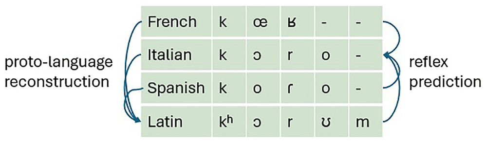
Figure 1. Schematic illustration of reflex prediction and proto-form reconstruction as similar tasks.
Reflex prediction infers descendant forms from related languages; proto-form reconstruction infers the etymon from descendant reflexes.
The reconstruction of proto-languages allows us to get a deeper understanding of the evolution of languages and language families and gives us insights into human pre-history (e.g. Anthony, 2007; Heggarty et al., 2023). Reflex prediction, on the other hand, could be used to facilitate language acquisition (Beinborn et al., 2013) and has been successfully employed to elicit word forms in fieldwork scenarios (Blum et al., 2024; Bodt & List, 2021).
Recent work
In recent years, a range of methods have been proposed for the tasks of automatic phonological reconstruction and reflex prediction. These approaches can generally be divided into two categories: unsupervised and supervised. Unsupervised models try to predict etymons or reflexes using only the reflexes found in descendant or related languages—essentially following the traditional comparative method. Supervised methods, on the other hand, require annotated examples from the languages they are trained on in order to learn patterns of sound change and make predictions.
Bouchard-Côté et al. (2013) proposed a probabilistic model of sound change capable of unsupervised proto-language reconstruction, showing very promising results on a dataset of Austronesian languages. Another largely unsupervised method was presented by Jäger (2019), who aligns cognate sets using multiple sequence alignment (MSA) and then performs ancestral state reconstruction column by column to reconstruct the proto-sounds. MSAs in the context of historical linguistics refer to the process of aligning cognates to identify sound correspondence patterns, which are ideally reflected in the columns of the alignment. Both of these unsupervised approaches rely on phylogenetic information, which is either inferred from the data itself (see also Jäger, 2022) or provided in advance.
So far, however, very few fully unsupervised methods have been proposed (cf. List, 2024). By contrast, there are many more approaches to supervised automatic phonological reconstruction. These can be roughly split into two main types: encoder-decoder architectures and position-wise classifiers. Figure 2 depicts the simplified structures of both approaches. Encoder-decoder models process the context—cognate sets in this case—through an encoder and then generate the target form character by character using an autoregressive decoder. This means each character prediction is conditioned not only on the input cognate set, but also on the model’s own previously generated outputs. In position-wise classifiers, each character is predicted based on the given context for the respective position and independent of the other predicted characters.
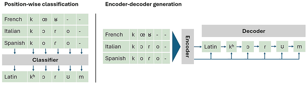
Figure 2. Comparison of position-wise classification and encoder-decoder architectures.
In position-wise classification (left) each position of the target is predicted independently of the other predicted positions. In encoder-decoder architectures (right) the target is sequentially generated, with each prediction informing subsequent predictions in addition to the context (cognate set).
Most position-wise methods apply MSA beforehand so that corresponding characters are aligned across languages. A representative example is the method by List et al. (2022b), which also includes a trimming step: characters in the proto-form that have no reflexes in the daughter languages (such as the word-final /m/ in Latin in Figure 1) are prepended to the following characters (or appended in the case of word-final characters). This prevents the model from having to infer a sound from an alignment column consisting solely of gaps (see also Blum & List, 2023). Additionally, the authors enriched each position in the alignment with positional and prosodic information. Each position is then predicted using a support vector machine (SVM; Cortes & Vapnik, 1995), achieving near state-of-the-art results for phonological reconstruction at the time.
As mentioned earlier, proto-form reconstruction and reflex prediction are closely related tasks. Accordingly, the model by List et al. (2022b) was also successfully used as a strong baseline in the SIGTYP 2022 Shared Task on cognate reflex prediction (List et al., 2022c). The overall best-performing model in that task was presented by Kirov et al. (2022), who framed the reflex prediction task as an image inpainting task (see Liu et al., 2018). Here, each character of a cognate set becomes a pixel in an image, with one fixed row per language. By removing words (i.e., rows of pixels) and thus masking parts of the image, the model learns to predict the missing characters based on the information found in surrounding context. One advantage of this model is that it learns structural relationships between characters across languages using convolutional layers and without needing to pre-align the input.
Akavarapu & Bhattacharya (2023) apply MSA and trimming to the cognate sets and pass them through the MSATransformer (Rao et al., 2021), a model originally developed for protein sequence alignments. This model applies attention across both rows and columns of the MSA, capturing language-internal and cross-linguistic structure alike. The authors then predict characters for each position in the alignment, yielding state-of-the-art results on both reflex prediction and proto-language reconstruction. Unlike most other approaches, the model is trained on multiple datasets simultaneously. This enables the model to learn cross-linguistically informative patterns of sound change, which is beneficial in light of data scarcity. By re-using the datasets used by List et al. (2022b) and the Shared Task (List et al., 2022c), the authors establish a useful benchmark for both tasks, with their strong results serving as baseline in the work at hand.
A prominent encoder-decoder model for proto-form reconstruction is the neural translation model (NMT) by Meloni et al. (2021), which uses a recurrent neural network (RNN) in both parts of the model, with the addition of attention in the decoder (see Bahdanau et al., 2016). The input consists of concatenated cognates from the daughter languages, with language information added to each character. The model, trained on the Romance dataset by Dinu & Ciobanu (2014), yielded promising results in reconstructing Latin forms. Building on this, Kim et al. (2023) developed a Transformer-based encoder-decoder model (Vaswani et al., 2017), using a similar workflow and achieving slightly better results. The main issue with these and related approaches (e.g., Cui et al., 2024; Fourrier et al., 2021; Lu et al., 2024a; Lu et al., 2024b) is that they rely on relatively large datasets—such as the Romance (Dinu & Ciobanu, 2014) or Chinese (Chang et al., 2022) datasets—which do not reflect the typical data scenarios found in historical linguistics (cf. List, 2024).
Contribution
Models for proto-language reconstruction and reflex prediction, such as the ones presented above, typically rely on mappings from characters to discrete symbols. However, over 8,000 distinct speech sound have been defined and used across different datasets (see List et al., 2024), and many of these occur only in a few languages. As a result, models often see such rare symbols too infrequently to learn meaningful relationships between sounds. This is also due to the conversion of sound representations to nominal identifiers in most machine learning models, which ignores any inherent phonological similarity between them.
One way to address the sparsity would be to convert the symbols to more limited inventories, such as simplified IPA representations (e.g. without diacritics), ASJP (Wichmann et al., 2016) or Dolgopolsky sound classes (Dolgopolsky, 1964), reducing their sizes to sometimes less than 100 symbols in total. This, on the other hand, is impractical for an accurate phonological reconstruction, as many important distinctions are lost and it is therefore not typically done for the task of proto-language reconstruction or reflex prediction.
In this paper, I introduce a method that circumvents the sparsity issue without sacrificing detail of phonological representation: instead of relying on discrete character-symbol mappings, it uses phonological feature vectors as character representations. This approach offers two main benefits. First, it directly encodes phonological similarity, grouping similar sounds closer in vector space. Second, and more crucially, each feature is observed across many characters, helping the model generalize better to rarely encountered sounds.
To test the effectiveness of this representation, I present a simple Transformer-based encoder-decoder model, the Feature Vector Transformer (FeVeT), and show that it achieves competitive, state-of-the-art results in both reflex prediction and proto-form reconstruction— surpassing the baseline established by Akavarapu & Bhattacharya (2023). All code, data and the results of the analyses can be found in the underlying data (Wientzek, 2025).
The remainder of this paper is structured as follows: Section 2 presents the workflow, covering data preparation, the model architecture, which datasets were used and how the model was trained and evaluated. Section 3 reports the results, followed by discussion and conclusions in Sections 4 and 5.
Methods
Data preparation
Each input to the model consists of a cognate set. Since the model employs an attention-based decoder for autoregressive output generation instead of position-wise predictions, multiple sequence alignment or trimming is not applied. Instead, the decoder attention is expected to learn a soft alignment over the input cognates, weighting the importance of each segment dynamically (see 'Model').
The key difference to previous architectures is the input encoding: instead of mapping each character to a discrete class, they are represented as a feature vector using the SoundVectors Python package (Rubehn et al., 2024). These ternary feature vectors consist of 39 phonological features such as [consonantal], [hitone], or [back]. This allows for the representation of the majority of the >8000 IPA sounds in the Cross-Linguistic Transcription Systems collection (CLTS; List et al., 2024) with unique feature vectors, while duplicate mappings still retain a linguistically meaningful structure.
Each position in the vector can take a value of 0 ("does not apply"), 1 ("not applicable"), or 2 ("applies"). For example, a vowel would be assigned a 1 for the [hitone] feature, since tone features are only applicable to tonal segments.
To mark learnable word boundaries, a [SEP] (separator) token is appended to each reflex form. To handle the special symbols [SEP] and [PAD] (padding), the space of possible feature values is extended beyond the original ternary set by adding two classes. These tokens are represented by vectors filled with their respective values—i.e., a vector of all 3s for [SEP] and all 4s for [PAD]—such that they can be processed in the same way as the character feature vectors by the model.
Although no real sound corresponds to a vector of uniform values (e.g., all 2s), this encoding ensures special tokens remain distinct from valid phonological inputs and avoids overloading the model’s representation space with ambiguous tokens (e.g. having the features [+cons] and [+tense] simultaneously).
In addition to the cognate sequences, language information is also passed to the model as an auxiliary input. Each language is mapped to a numerical class, and this language token is repeated for every segment in the respective reflex, mirroring the structure of the cognate set. From each cognate set, one word is selected to serve as the target for reconstruction, along with its language identity. The remaining cognates and corresponding language tokens in the set are padded to the same length (see Figure 3).
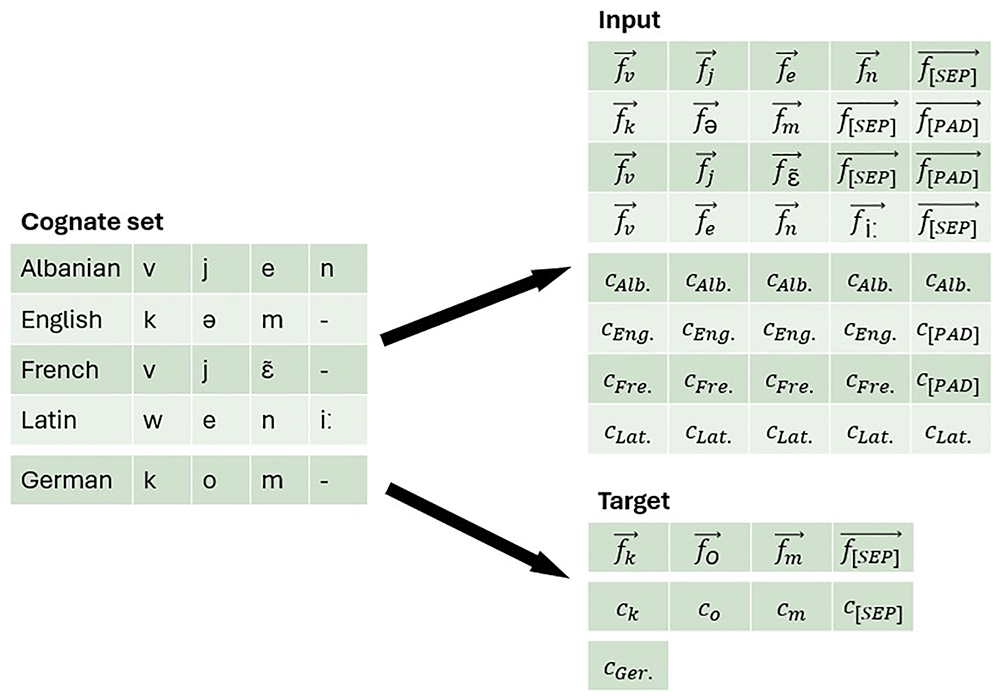
Figure 3. Example of model input preparation.
The figure illustrates the input and target structure based on an example from the kesslersignificance dataset (Kessler, 2021). A cognate set (left) is separated into inputs (top right) and a target (bottom right). Input consists of two matrices: (1) the feature vector representation , where x stands for either IPA or special characters, and (2) class IDs ci, where i stands for IPA and special characters, as well as languages. The target consists of the reflex of the focus language (here: German), represented both as a sequence of phonological feature vectors and as class IDs. The goal of the model is to predict the target reflex form based on the input context.
Because multiple IPA symbols can share identical or near-identical feature vectors, predicting features alone can result in ambiguous reconstructions. To avoid this, the model is trained to predict both the phonological feature vectors and the corresponding IPA class indices, ensuring interpretable outputs. This proved more effective than attempting to reconstruct IPA characters directly from predicted feature vectors in a post-processing step.
Model
The model consists of a Transformer encoder and decoder, implemented using the standard PyTorch modules (Paszke et al., 2019). The model description outlined below is depicted in Figure 4.
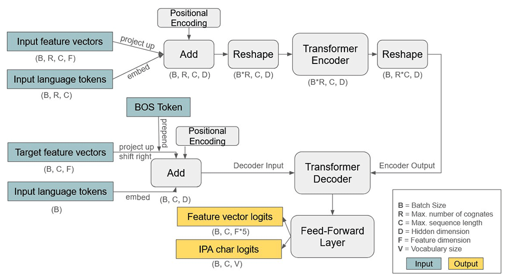
Figure 4. FeVeT model architecture overview.
Architecture of the Feature Vector Transformer (FeVeT) model for reflex prediction and proto-form reconstruction. Each reflex in a cognate set is encoded as a sequence of phonological feature vectors, enriched with language embeddings and positional encodings. These are passed through a Transformer encoder. The encoded reflexes are concatenated into a single context sequence for the Transformer decoder, which receives a shifted version of the target sequence during training (teacher forcing) and autoregressively generates outputs during inference. At each decoding step, the model predicts both a phonological feature vector and a corresponding IPA character. The decoder is conditioned on the target language via language embeddings.
Each input character is initially represented by its feature vector. These vectors are projected into a higher-dimensional embedding space. The language token sequences are encoded via learned embeddings of the same dimensionality as the up-projected feature vectors and are added to them. This integration allows the model to distinguish between the same phonological segments occurring in different languages (cf. Meloni et al., 2021). Additionally, language embeddings may enable parameter sharing across similar languages, which is especially useful in low-resource scenarios.
As is standard in attention-based architectures, each embedded position is enriched with positional encodings, since both the Transformer encoder and decoder lack inherent awareness of sequence order (Vaswani et al., 2017).
The input sequences—now enriched with both language and positional information—are passed individually through the encoder. To avoid the encoder processing padding tokens, standard masking is applied. Once encoded, the outputs of all reflexes in a cognate set are concatenated to form a single sequence, which serves as the context for the decoder.
Training uses standard teacher forcing (Williams & Zipser, 1989), where the decoder receives the gold feature vectors (i.e., the reflex to be reconstructed) shifted right, prepended with a learnable [BOS] (beginning-of-sequence) token, and enriched with language and positional information. A causal mask ensures that the decoder attends only to previous positions during prediction. This ensures that the decoder does not base its predictions solely on possibly incorrect previously generated outputs, but instead always has access to the ground-truth feature vectors during training—allowing the model to converge more quickly.
Each decoding step produces both:
1. a feature vector, where each position is predicted independently as a classification over the five possible values (0: does not apply, 1: not applicable, 2: applies, 3: [SEP], 4: [PAD]), and
2. an IPA character ID, corresponding to a discrete symbol in the output alphabet.
During inference, the decoder receives the encoded input and the [BOS] token, and generates outputs autoregressively. The decoder outputs at each step are passed through a classifier and the most likely value for each position in the predicted feature vector is selected, forming the next vector input. This newly generated vector is concatenated to the previous outputs, together serving as the next input sequence for the decoder.
To ensure that the IPA characters generated in the decoding steps are linguistically meaningful, they are incorporated directly into training. That is, the classifier operates in two steps: first, the subsequent feature vector representation is predicted via a feed-forward network using the decoder output as input. Secondly, another feed-forward layer is used to predict a probability distribution over the IPA character vocabulary based on this vector. Therefore, during training the model outputs both the IPA characters and the feature vectors. For both these outputs, cross-entropy loss is calculated against the target IPA sequences and target feature vectors, encouraging the model to optimize both these representations.
Evaluation
To ensure comparability with prior work and because these metrics have proven effective in this domain, I report the Levenshtein Distance (Levenshtein, 1965), Normalized Levenshtein Distance, and the B-Cubed F-Score (Amigó et al., 2009).
Levenshtein Distance, often referred to as Edit Distance (ED), measures the minimum number of insertions, deletions, and substitutions required to transform one word into another. Since longer words naturally allow for more edit operations, they tend to have higher ED values. For this reason, ED is often complemented or replaced by the Normalized Edit Distance (NED), which divides the raw edit distance by the length of the longer of the two compared words.
In contrast, the B-Cubed F-Score (BC) is a measure adapted from clustering evaluation and can be used to evaluate the structural similarity between sequences (List, 2019b). Because it emphasizes structural consistency, BC is more tolerant of systematic errors than raw edit-based metrics. For example, if a model consistently predicts [k] instead of [g], this is penalized as a full substitution each time in ED (always +1), regardless of the underlying pattern. The BC, however, is more forgiving in such cases, as it is a consistent error. Therefore, while a BC of 1 indicates structural identity between the target and gold form, it does not necessarily imply a phonologically perfect reconstruction. For ED and NED, lower values correspond to a more accurate reconstruction.
All metrics are computed over the full set of predicted and gold forms per target language. The functions to calculate these metrics are available in the LingRex package (List & Forkel, 2023) for Python.
In addition to the metrics described above, this work also analyzes model error patterns. Unlike position-wise classifiers—where erroneous predictions can be directly identified by comparing aligned positions (as done, e.g., in Akavarapu & Bhattacharya, 2023)—error pattern extraction in encoder-decoder architectures is less straightforward. While Meloni et al. (2021) manually evaluated a subset of prediction errors, this approach is beyond the scope of the present work due to the time and labor required for such analysis. Therefore, an approximation based on aligning the predictions with the gold-forms is proposed, consisting of the following steps:
1. A custom scorer for pairwise Needleman-Wunsch alignment (Needleman & Wunsch, 1970), implemented in LingPy (List & Forkel, 2023), is created using the phonological feature vectors (inspired by List, 2019c). The similarity measure used in the scorer is the inverse of the normalized distances between the feature vectors, quantifying phonological dissimilarity. A feature changing from "applies" to "does not apply" (or vice versa) adds a distance of 1, while transitions involving "not applicable" add a distance of 2, reflecting broader categorical shifts (e.g., consonant vs. tone) rather than more localized distinctions such as place of articulation (e.g., [+back] vs. [-back]).
2. Using this scorer, predicted IPA sequences are aligned with the gold forms. The positional shifts of characters in the alignment are tracked for both prediction and label.
3. The tracked positional shifts are then used to replicate the alignment with the predicted feature vectors.
4. Using the aligned IPA sequences, error patterns can be computed. The same is done for the aligned feature vectors, allowing for detailed tracking of which features were incorrectly predicted and in what direction (e.g., voicing incorrectly added or removed). Gaps are not considered when comparing the aligned feature vectors.
Datasets
To ensure direct comparability with prior work, I use the exact same datasets and splits as Akavarapu & Bhattacharya (2023), who have established a strong baseline for both reflex prediction and proto-language reconstruction.
For the reflex prediction task, these are the dataset provided in the SIGTYP 2022 Shared Task (List et al., 2022c), which draws on a diverse set of Lexibank (List et al., 2022a) datasets, covering a variety of language families. During the task, the data was given out in two phases, training and surprise, with models being evaluated on the latter (Table 1). Following Akavarapu & Bhattacharya (2023), the model is evaluated on the 10%, 30%, and 50% test proportions of the surprise data given out in the shared task.
Table 1. Training and surprise datasets from List et al. (2022c) used in the reflex prediction task.
| Training | Surprise |
|---|
| Family | Languages | Words | Cognates | Family | Languages | Words | Cognates |
|---|
| Tshanglic | 8 | 2063 | 403 | Atlantic-Congo | 10 | 1218 | 388 |
| Bai | 9 | 5773 | 969 | Hui | 19 | 9750 | 518 |
| Sino-Tibetan | 7 | 1426 | 248 | Chapacuran | 10 | 939 | 187 |
| Sui | 16 | 10139 | 1048 | Western Kho-Bwa | 8 | 5214 | 915 |
| Uto-Aztecan | 9 | 771 | 118 | Berta | 4 | 600 | 204 |
| Afro-Asiatic | 19 | 2583 | 340 | Palaung | 16 | 1911 | 196 |
| Dogon | 16 | 4405 | 971 | Burmish | 9 | 2202 | 467 |
| Japonic | 10 | 1802 | 278 | Indo-European | 5 | 565 | 212 |
| Indo-European | 4 | 1320 | 512 | Karen | 8 | 2363 | 379 |
| Burmish | 7 | 2501 | 576 | Bai | 10 | 4356 | 658 |
| Total | 105 | 32783 | 5463 | Total | 99 | 29118 | 4124 |
For the proto-language reconstruction task, the datasets from List et al. (2022b) are used (Table 2), adopting the same proportions (10%, 50%, and 80%) for held-out test data as Akavarapu & Bhattacharya (2023). In line with their setup, these datasets are extended with all available data from the reflex prediction task to pre-train the model, excluding any forms from protolanguages.
| Family | Languages | Words | Cognates |
|---|
| Bai | 10 | 3866 | 459 |
| Burmish | 9 | 1711 | 269 |
| Karen | 11 | 3231 | 365 |
| Lalo | 8 | 7815 | 1251 |
| Purus | 4 | 693 | 199 |
| Romance | 6 | 18806 | 4147 |
| Total | 48 | 36122 | 6690 |
Proto-language reconstruction is evaluated using 10-fold cross-validation, following the exact splits publicly released by Akavarapu & Bhattacharya (2023). This ensures consistency and comparability across models.
Training regime
During training, each batch consists of randomly sampled cognate sets from the training data. From each set, one reflex is randomly selected to serve as the prediction target, while the remaining cognates provide context. For every epoch, 500 batches of size 48 are sampled in this manner. Because sampling is done without constraints, some cognate sets may be selected multiple times within a single epoch, while others may not be selected at all. Similarly, the same word may be chosen as target multiple times, while others might never serve as targets. This introduces some imbalance in target frequency but improves robustness by exposing the model to varied training data across epochs.
Reflex prediction task
For the reflex prediction task, the model is trained for 32 epochs using the AdamW optimizer (Loshchilov & Hutter, 2019) from the PyTorch library with a learning rate of 5e-4 and default settings. The architecture consists of 1 Transformer encoder layer and 2 Transformer decoder layers, each with 4 attention heads. The hidden size is set to 256.
Following initial training, fine-tuning is applied on each individual dataset. This consists of 8 additional epochs with 100 steps each and a reduced learning rate of 1e-4. The model is evaluated on the data splits given out during the SIGTYP 2022 Shared Task (List et al., 2022c). The results are reported both for the run with and without fine-tuning step, as well as for a model variant that uses IPA characters instead of feature vectors as input and otherwise unchanged settings.
Proto-Language reconstruction task
For proto-language reconstruction, the model is pre-trained on all available data (see 'Datasets') in the same manner as for the reflex prediction task, but with a learning rate of 1e-3 and a hidden size of 128. Then, fine-tuning is applied individually for each dataset in the protolanguage reconstruction task over 40 epochs, using a batch size of 48 and a learning rate of 5e-4. For the 0.8 test proportion, where for some datasets the available number of cognate sets during training is less than 100, the batch size is reduced to 16. This allows for more gradient updates per epoch, improving the capability of the model to generalize (Goodfellow et al., 2016), and lead to a slight boost in performance during experiments.
For model training and testing, the splits from the 10-fold cross-validation provided by Akavarapu & Bhattacharya (2023) are used. Since only proto-forms are predicted, there is no need to randomly sample targets within each set.
In addition to the three test proportions, the model was also tested on the zero-shot condition. This setting resembles an unsupervised reconstruction scenario, where the model must infer proto-forms purely from reflex patterns, without ever being exposed to a gold proto-form. The results are reported for these conditions as well as for the model without pre-training on the reflex prediction task data but trained only on the task-related datasets from List et al. (2022b).
No exhaustive hyperparameter tuning was carried out, as this would have been computationally intensive. Instead, settings were selected based on prior experience with similar architectures and preliminary results. Model training was performed on a notebook equipped with an NVIDIA GeForce RTX 3070 GPU and pre-training on all available data takes approximately 10 minutes.
Results
Model performance
The average model performance on the reflex prediction task and the proto-language reconstruction task is summarized in Table 3 and Table 4. Detailed results by language and language family are provided in the underlying data (Wientzek, 2025).
Table 3. Comparison of model performances on the reflex prediction task.
Comparison of FeVeT with and without fine-tuning, the variant using only IPA characters as input (IPA-only) and CognateTransformer (Akavarapu & Bhattacharya, 2023) using three metrics: Edit Distance (ED), Normalized Edit Distance (NED), and B-Cubed F-Score (BC). Lower ED and NED and higher BC indicate better performance. Bold values indicate the best performance for a test proportion.
| Proportion | Model | ED (↓) | NED (↓) | BC (↑) |
|---|
| 0.1 | CognateTransformer | 0.8966 | 0.2421 | 0.7823 |
| FeVeT (no fine-tuning) | 0.9451 | 0.2525 | 0.7704 |
| FeVeT | 0.7836 | 0.205 | 0.8041 |
| IPA-only | 2.559 | 0.6364 | 0.5162 |
| 0.3 | CognateTransformer | 1.1235 | 0.2919 | 0.6954 |
| FeVeT (no fine-tuning) | 1.1046 | 0.2837 | 0.6874 |
| FeVeT | 0.9589 | 0.2397 | 0.7232 |
| IPA-only | 2.511 | 0.6261 | 0.4764 |
| 0.5 | CognateTransformer | 1.2786 | 0.3332 | 0.6477 |
| FeVeT (no fine-tuning) | 1.2405 | 0.3222 | 0.6426 |
| FeVeT | 1.1111 | 0.2825 | 0.673 |
| IPA-only | 2.508 | 0.6642 | 0.4489 |
Table 4. Comparison of model performances on the proto-language reconstruction task.
Comparison of FeVeT with and without pre-training, its performance in the zero-shot condition (no proto-language data seen during training), and CognateTransformer (Akavarapu & Bhattacharya, 2023) using three metrics: Edit Distance (ED), Normalized Edit Distance (NED), and B-Cubed F-Score (BC). Lower ED and NED and higher BC indicate better performance. Bold values indicate the best performance for a test proportion.
| Proportion | Model | ED (↓) | NED (↓) | BC (↑) |
|---|
| 0.1 | CognateTransformer | 0.7459 | 0.1595 | 0.8081 |
| FeVeT (no pre-training) | 0.6822 | 0.1512 | 0.8159 |
| FeVeT | 0.6248 | 0.1371 | 0.8278 |
| 0.5 | CognateTransformer | 0.8177 | 0.176 | 0.7534 |
| FeVeT (no pre-training) | 0.7568 | 0.1702 | 0.7585 |
| FeVeT | 0.7083 | 0.1559 | 0.7709 |
| 0.8 | CognateTransformer | 0.9754 | 0.2142 | 0.7132 |
| FeVeT (no pre-training) | 0.9828 | 0.225 | 0.6999 |
| FeVeT | 0.9115 | 0.2055 | 0.7174 |
1.0
(zero-shot) | CognateTransformer | 2.6477 | 0.5758 | 0.5499 |
| FeVeT | 2.6774 | 0.5794 | 0.5424 |
For the reflex prediction task, results for FeVeT without fine-tuning on individual datasets, as well as for a variant of the same architecture trained only on IPA characters instead of feature vectors ('IPA-only') are also reported. FeVeT outperforms the current state-of-the-art across all test proportions and metrics. Without fine-tuning, it performs comparably or only slightly worse (notably for the 0.1 test proportion). The model using only IPA characters as input (IPA-only) performs substantially worse across all proportions, highlighting the importance of feature representations for this model architecture.
For the proto-language reconstruction task, I further include comparisons with a FeVeT model trained without pre-training on the reflex prediction task data, as well as a zero-shot learning scenario in which no proto-language data is seen during training (equivalent to a 1.0 test proportion). While FeVeT again achieves better performance across nearly all test proportions, the improvements diminish as the amount of proto-language data available for training decreases. In the zero-shot setting, FeVeT performs slightly worse than the CognateTransformer, though results remain comparable and fall within model variance. Pretraining consistently improves performance across all conditions, but even without the model achieves competitive results.
Model errors
As described in the Methods section, model errors are analyzed with respect to sound correspondences by aligning the gold forms with the model predictions. As done by Akavarapu & Bhattacharya (2023), I specifically investigate errors in the proto-language reconstruction task at the lowest and highest test proportions, i.e., 0.1 and 0.8. To ensure comparability, also the same normalization strategy was adopted: first, the relative error rates are computed for each language family, then these rates are aggregated and normalized. This is necessary due to varying dataset sizes and error types across families—Romance, for example, constitutes nearly half the data and could otherwise skew the distribution with its more frequently occurring error types such as vowel lengths (cf. Meloni et al., 2021).
In addition to character-level correspondence errors, model errors are also analyzed at the level of phonological features. Table 5 shows a distribution of errors grouped by broader classes. The 15 most common errors for test proportion 0.8 are summarized in Table 6. The detailed lists of errors across all test proportions and for individual language families can be found in the underlying data (Wientzek, 2025).
Table 5. Distribution of error categories in the proto-form reconstruction task for test proportions 0.1 and 0.8.
Test
Proportion | Deletion | Insertion | Tones | Both
vowels or
glides | Both
consonants | Mixture of
vowel/glides and
consonants | Dipthongs |
|---|
| 0.1 | 0.1574 | 0.068 | 0.0909 | 0.3046 | 0.3476 | 0.0168 | 0 |
| 0.8 | 0.1307 | 0.0833 | 0.1073 | 0.3317 | 0.3047 | 0.0151 | 0 |
Table 6. Most frequent phonological feature prediction and character-level errors observed in the 0.8 test condition of the proto-form reconstruction task.
| Feature vectors | IPA characters |
|---|
| Feature | Gold | Prediction | Proportion
(normalized) | Gold | Prediction | Proportion
(normalized) |
|---|
| hi | - | + | 0.0629 | p | b | 0.0222 |
| front | + | - | 0.0475 | o | u | 0.0207 |
| hi | + | - | 0.0465 | j | - | 0.0176 |
| lo | + | - | 0.0456 | u | o | 0.0141 |
| front | - | + | 0.0411 | ʔ̚ | ʔ | 0.014 |
| hitone | + | - | 0.0354 | ³ | ² | 0.0138 |
| back | + | - | 0.0352 | h | - | 0.0133 |
| loreg | - | + | 0.0341 | ³ | ¹ | 0.0129 |
| long | + | - | 0.0321 | a | ɨ | 0.0128 |
| tense | - | + | 0.0316 | - | r | 0.0121 |
| tense | + | - | 0.0292 | a | - | 0.0118 |
| lo | - | + | 0.0272 | i | ɨ | 0.0115 |
| voi | + | - | 0.0248 | r | j | 0.0112 |
| loreg | + | - | 0.0226 | k | g | 0.0108 |
| back | - | + | 0.019 | ɔ | o | 0.0104 |
As seen in both the feature and character level, errors involving tongue movement—hence also vowel placement in the vowel space—are among the most frequent (e.g., [-hi] to [+hi], as in /u/ → /o/ or /r/ → /j/; also including [lo], [front], and [back]). Predictions involving sound length ([long]; mostly vowel length) and vowel tenseness ([tense]) are also commonly observed. Tone features, such as [hitone] and [loreg] (e.g., /²/ with [-hitone, -lowreg] vs. /³/ with [+hitone, +lowreg]), appear relatively frequently as well. Tones account for around 10% of the errors across all test proportions, matching the findings of Akavarapu & Bhattacharya (2023). This is not unexpected, given that four of the six datasets in this task contain tone languages.
While the error patterns presented here are largely consistent with those reported by Akavarapu & Bhattacharya (2023), two key differences are observable:
1. Insertions and deletions constitute a substantial portion of the errors, as also noted for the encoder-decoder models by Meloni et al. (2021) and Kim et al. (2023). These types of errors account for approximately 22% of all errors, regardless of test proportion.
2. Diphthongs, which are treated as units, are virtually absent among the model’s errors.
A further noteworthy observation concerns feature prediction errors involving non-applicable (NA) values. These occur when the model predicts a value for a feature that should be undefined for a particular sound, or vice versa. While relatively rare overall, such errors are most common for the features [ant], [distr], and [strid] (anterior, distributed, and strident; see Zsiga, 2013, pp. 265–266 for detailed definitions). Apart from the feature [tense], which is only defined for vowels, and tone- or diphthong-related features, which are undefined for all non-tone and non-diphthong sounds, respectively, these three represent the only features defined only for a subset of consonants (e.g., not for plosives). This partial applicability may contribute to increased difficulty in learning these features, as they represent less sharply defined class boundaries.
Figure 5 presents a heatmap of co-occurrences in feature prediction errors, with the value corresponding to the normalized proportion with regards to all pairwise mispredictions. The features [ant] and [distr] are most frequently mispredicted together. This is explained by the above-mentioned fact that these features are defined for the same subset of consonants and thus are often wrongly assigned a value or NA by the model together. The plot also reveals a stronger concentration of co-occurring errors among features relevant to vowel articulation and tongue positioning—namely [hi], [lo], [front], [back], [tense], and [round]. However, it should be noted that the level of error co-occurrence is generally low and subtle errors in predictions are a lot more common. Taking for example the errors in Table 6 where both sounds are vowels, none of the predicted sounds differ from the gold sound in more than one feature.
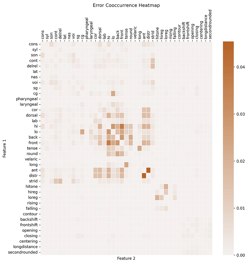
Figure 5. Heatmap of co-occurring feature prediction errors in the proto-form reconstruction task (test proportion 0.8).
Each cell indicates the normalized proportion of times two features were mispredicted together in the same segment. Darker colours correspond to higher frequencies of co-occurrences.
Another difficulty for the model can be seen in the plot: the differentiation between fricatives and affricates. For instance, the features [strid] (strident; only applicable for fricatives and affricates), [delrel] (delayed release; [+delrel] for affricates, [-delrel] for all other sounds), and [cont] (continuant; [-continuant] for affricates, [+continuant] for fricatives)—thus, the features that differentiate between fricatives and affricates—are more commonly incorrectly predicted together.
Tone- and diphthong-related features appear well-separated from vowel and consonant features. Errors in features from the tone cluster ([hitone] through [contour]) exclusively cooccur with other tone-related errors, while diphthong-related features ([backshift] through [secondrounded]) draw a similarly sharp boundary. This indicates that the model has largely succeeded in treating these groups as structurally distinct from other sound classes.
Overall, the sparsity of the heatmap suggests that most phonological features are independently learned, with a limited set of expectable confusions arising primarily from overlapping definitional spaces or articulatory proximity.
Learned rules of phonetic change
Some examples of sound changes learned—or not learned—by the model are presented in Table 7. All examples are taken from the Romance reconstruction task with test proportion 0.8. The model handles common and regular sound changes relatively well, such as the palatalization of /k/ before front vowels. It also tends to reconstruct word-final /m/ accurately, likely due to the predictability of its loss in that position. However, this sometimes leads to overgeneralization, with /m/ added where it does not belong (e.g., ɔfːɛrɛm instead of ɔfːɛrːɛ). In contrast, the loss of /h/—which occurred in all positions across the daughter languages—was rarely recovered (cf. Meloni et al., 2021).
Table 7. Examples of sound changes captured or missed by the model in Romance data.
| Examples | Rule | Rule application |
|---|
French: selebʁasjɔ̃
Italian: tʃelebratsjone
Spanish: θeleβɾaθjon
Latin: kɛlɛbraːtjoːnɛm
Prediction: kɛleːbraːtjoːnɛm | Palatalization
/k/ > [s ~ θ ~ tʃ] / _ {e, ɛ, i} | Mostly correct |
French: ʁepʁeɑ̃sibl
Italian: reprensibile
Portuguese: ʁepɹieɪŋsivɛl
Spanish: repɾensiβle
Latin: rɛprɛhɛnsɪbɪlɛm
Prediction: rɛpreːnsɪbɪlɛm | Loss of /h/
/h/ > ∅ | Mostly wrong |
French: edi
Italian: editːo
Portuguese: editʊ
Romanian: edikt
Spanish: eðikto
Latin: eːdɪktʊm
Prediction: eːdɪktʊm | Loss of final /-m/
/m/ > ∅ / _# | Mostly correct |
French: ublie
Italian: obljare
Portuguese: ɔlvidaɹ
Romanian: ujta
Spanish: olβiðaɾ
Latin: ɔbliːwɪskiː
Prediction: ɔblɪtaːrɛ | Metathesis
/bl/ > /lv/ or /lβ/ (Ibero-
Romance; irregular) | Conditionally correct
(mostly dependent
on cognates without
metathesis being
available) |
As also observed by Akavarapu & Bhattacharya (2023), metathesis, the change in the order of sounds, is a difficult sound change pattern for automated reconstruction. This is also true for the model at hand, despite not relying on predefined alignments, especially because metathesis does not occur regularly within most languages. For instance, the metathesis /bl/ > /lv/ or /lβ/ found in some Ibero-Romance languages is captured in the example shown in Table 7. However, it does not appear in cases like Latin ɔblaːtjoːnɛm (Spanish: oβlaθjon, Portuguese: ɔblɐsɐ̃ʊ̃) or Latin ɔblɪtːɛraːrɛ (Spanish: oβliteɾaɾ, Portuguese: ɔblitɨɾaɹ), where no such reordering occurs. Therefore, when removing the French and Italian cognates in the example from Table 7, the model reconstructs ɔlwɪaː instead of the correct ɔbliːwɪskiː, ignoring the metathesis. In contrast, it correctly predicts the sound order when either or both are present. These examples were selected to illustrate the types of correspondences the model is capable of learning, though more systematic frequency analysis is left for future work.
Discussion
Despite its conceptual simplicity, the model presented here outperforms the previous state of the art and overcomes key weaknesses found in comparable encoder-decoder architectures. The key innovation is the use of phonological feature vectors, which provide the model with a much more granular and linguistically meaningful representation of phonological segments. Rather than treating a sound change, e.g. from [a] to [u], as a switch between opaque symbol classes, the model can interpret such shifts as changes in specific features like [back] or [round]. While token-based models may learn to approximate such abstract relationships through high-dimensional embeddings, feature vectors offer a more transparent and linguistically grounded input representation, potentially resulting in more accurate model initialization and learning.
This representation also offers the potential for better generalization across language families. Because transitions between phonological features (e.g., [+voiced] to [-voiced], [-round] to [+round]) are typologically universal, the model can more easily capture cross-linguistic patterns than if it were restricted to transitions between individual IPA symbols—many of which may only appear in a narrow set of languages or contexts. The effectiveness of using feature vectors in this model architecture is clearly demonstrated in the comparison with the results of the same model using only IPA characters as input, which performs significantly worse (see Table 3).
Furthermore, encoder-decoder architectures such as the one used here have a key structural advantage over position-wise classifiers (e.g. Akavarapu & Bhattacharya, 2023; List et al., 2022b): they do not rely on a predefined output structure. Previous state-of-the-art approaches relied on multiple sequence alignments combined with trimming strategies to constrain the output space, especially where specific positions were difficult to predict. In scenarios where the form to be reconstructed is not known in advance, such methods are limited by their reliance on strong structural assumptions.
In theory, the use of feature vectors opens the possibility of predicting entirely novel sounds, i.e. sounds not observed in the training data. Instead of outputting IPA characters, the model could output only the feature vectors, which are then mapped to the closest sounds found in collections of IPA symbols like CLTS in a post-processing step. Although this approach was found to be suboptimal for the task at hand due to the lack of one-to-one mappings between feature vectors and all IPA characters, it may be better suited to a more controlled setting, such as the case study by Hartmann (2019), where the aim was to reconstruct the exact phonetic quality of certain Proto-Indo-European sounds.
Certain modelling choices proved surprisingly impactful in the design and performance of the model. For instance, unlike in Meloni et al. (2021) and Kim et al. (2023), the input cognate were not concatenated before encoding, but only after, leading to significantly better results. Although one might expect the encoder’s self-attention to identify useful cross-linguistic patterns, the results suggest that this role is largely handled by the decoder. The encoder, by contrast, may primarily serve to model intra-lingual structure. Indeed, I found that replacing the encoder with either convolutional or recurrent layers led to only marginal performance drops, indicating that attention on both sides may be redundant and that the decoder handles the processing of cross-linguistic information well enough. The model generally showed high sensitivity to such architectural decisions and overfitting, as is reflected in the minimal setup of only one encoder layer and two decoder layers, with more decreasing the performance.
I also experimented with imputing missing reflexes in the proto-language reconstruction task. After pre-training and a brief fine-tuning phase, the model was used to predict missing forms in the training data, thereby providing a more complete context for each cognate set. Here, it did not matter whether the cognate still existed in the language with the missing form, but rather what form it would have if it existed. Using these now 'complete' datasets, another round of finetuning was performed, to then predict the proto-forms in the test sets. However, this approach neither improved nor degraded performance. I also tested imputing the missing reflexes in the test sets (i.e., the context used to predict the proto-form), and both in the training and test sets, with the same result. The most plausible explanation is that the benefits of a more complete context were outweighed by the biases introduced through imperfect predictions.
While FeVeT outperforms the current state-of-the-art CognateTransformer (Akavarapu & Bhattacharya, 2023), the differences are more marginal in the proto-language reconstruction task under a high test-data proportion (0.8). A notable difficulty for the model in this hard setting could stem from the language tokens, which are used to condition the decoder on predicting the form for a specific language. In the reflex prediction task, the model can learn language embeddings through repeated exposure to the relevant tokens in both encoder and decoder inputs. However, in proto-language reconstruction, the encoder is never exposed to the token of the proto-language it is asked to predict, as it is never part of the input but only constitutes the target. As a result, it is difficult for the decoder to learn a meaningful embedding for the target proto-language solely based on, in some datasets, only the few dozen examples available in the 0.8 test proportion. In these cases, the model relies more strongly on generalizations from learned patterns in other languages, which may also be why the impact of pre-training is more noticeable here. This limitation becomes particularly visible in the zero-shot setting, where the proto-language token is completely missing in the training data and the prediction cannot be meaningfully conditioned.
It should be noted that for the zero-shot and IPA-only configurations, the hyperparameters were not adjusted. Given the model's sensitivity to parameters such as embedding size or learning rate, performance in these settings could likely be improved by tweaking the hyperparameters. However, this was beyond the scope of the present study and the results should nonetheless provide a reasonable approximation of the expected performance.
The comparison of the model's errors with Akavarapu & Bhattacharya (2023) reveals that while the types of errors made by both models are often similar, they are not entirely overlapping. Most notably, insertions and deletions account for roughly 22% of the total errors in the present model, yet are not even mentioned in their analysis. This discrepancy suggests that combining the strengths of an encoder-decoder model and position-wise classification might yield further improvements. Such integration could take the form of a hybrid model or ensemble models that combine outputs from different architectures. However, it should also be considered that at least some of the observed insertions and deletions may be artifacts introduced by the alignment procedure used for error analysis. Additionally, post-processing strategies enforcing phonotactic constraints could be explored to correct implausible output sequences and further reduce error rates.
Regarding the observed sound change rules learned by the model for the Romance dataset, it becomes apparent that irregular changes and missing sound reflexes remain challenging for automatic reconstruction. The model’s more reliable predictions of palatalization and word-final /m/ loss—despite this segment being absent in all reflexes—likely stem from the regularity of both phenomena. In contrast, /h/ loss, though equally consistent across the daughter languages, lacks clear phonotactic cues, making it harder to recover. Similarly, metathesis presents a challenge: as an irregular and often language-specific phenomenon, it may also fall outside the generalizable scope of the training data due to the model’s lack of strong alignment cues or recurrent cross-linguistic patterns. Some of these issues may again be addressed by employing the model extensions discussed above.
In the study at hand, the goal was to ensure comparability to the baseline set up by Akavarapu & Bhattacharya (2023) and therefore the inclusion of additional external data was avoided. However, several promising approaches for future improvement can nonetheless be identified.
While pre-training contributes modestly to overall performance, a more targeted selection of pre-training data may help strengthen its impact. Specifically, it would be worthwhile to explore whether it is possible to determine which datasets are informative for transfer learning—i.e., which provide useful patterns for reconstructing a specific (proto-)language—and which merely introduce noise. This could enable the use of the entire Lexibank (List et al., 2022a) collection consisting of over 70 datasets, with a pre-selection mechanism identifying only those datasets that are most beneficial for, say, reconstructing Proto-Burmish. Another area for improvement lies in the use of language embeddings. These are essential for conditioning the model on a specific prediction target, but in low-resource scenarios, these embeddings may not be meaningfully learned. One possible solution is to initialize these embeddings with external information, such as cophenetic distances derived from the Glottolog (Hammarström et al., 2025) tree. Ultimately, the goal would be to develop a model capable of accurate zero-shot prediction, which would be comparable to a unsupervised reconstruction scenario (cf. List, 2024). While such a model is not yet achievable with current methods, both more carefully executed pre-training and the incorporation of linguistically informed language embeddings represent promising steps in that direction. These measures would allow the model to make better use of cross-linguistic information and more effectively capture evolutionary relationships between languages.
Conclusion
In this study, I introduced FeVeT, a simple, fast, and scalable Transformer-based model architecture for supervised reflex prediction and proto-language reconstruction. Despite its minimal configuration, the model achieves results comparable to or surpassing the previous state of the art. The core innovation lies in the use of phonological feature vectors to represent input characters, providing a more granular and linguistically informed encoding. This representation helps the model address data scarcity more effectively and facilitates better generalization across language families.
Ultimately, the model presented here serves as a proof of concept for the effectiveness of phonological feature vectors in this domain. Future work could likely yield additional improvements by exploring different architectures tailored to this input representation, implementing more targeted pre-training strategies or incorporating more structured information about language relationships.
At the same time, it is important to emphasize that, as a supervised model relying on already reconstructed proto-forms, models like FeVeT cannot replace the work of trained historical linguists. Their role should be understood as that of an assistant—supporting faster reconstructions, facilitating exploratory analyses, or serving as a tool for sanity checks and validation.









