Introduction
Given ongoing and accelerating global climatic change1, and our current climate emergency2–4, the need for robust methodologies to assess impacts on terrestrial ecosystems5 and associated biological6 and human systems7, is ever more relevant and increasingly more urgent. Environmental stratification, or more specifically, the “EnS” environmental stratification methodology8–11 provides a structured approach to modeling interactions between climate variables and terrestrial landscapes. This method is, among other equally relevant applications, well suited to analyzing potential changes in vegetated landscapes12, where shifts in temperature, precipitation, and other bioclimatic factors can influence ecosystem structure13 and function14,15. The integration of environmental stratification with predictive modeling, combined with parameterization and validation from a variety of thematically or geographically specific empirical or modeled datasets16, can provide an improved understanding of how climate change and shifting bioclimatic conditions may alter ecological patterns and processes for both natural13,17 and managed systems9. Understanding these changes in ecological processes is fundamental to developing effective human adaptation strategies to climate change18.
Ecosystems respond dynamically to shifting bioclimatic conditions5, influencing biodiversity, ecosystem services, and resource availability, which in turn affect human societies6. By integrating predictive modeling with ecological monitoring, policymakers and stakeholders can anticipate bioclimatic shifts and their impact on ecosystem structure and function19, allowing for proactive adaptation measures in biodiversity conservation20,21, agriculture22,23, water resource management24, rural development and urban planning18,19. For example, ecosystem-based adaptation strategies (EbA) and other Nature Based Solutions (NbS)25, such as restoring wetlands to mitigate floods or implementing agroforestry systems to enhance soil conservation26, have been shown to enhance both ecological and human resilience to climate stressors. However, integrating these approaches into appropriate policies requires a comprehensive approach and context-aware understanding27. Additionally, studies indicate that transformative adaptation, where fundamental changes in land use and resource management are implemented, can be necessary in regions experiencing extreme ecological shifts28. A predictive understanding of how climate change modifies future bioclimatic conditions29, and consequently interactions in social-ecological and other human systems18, leading to shifts in system trajectories, can help identify appropriate adaptation responses, including transformative adaptation, that provide long-term and sustainable benefits. Predictive and integrative modeling incorporating environmental and bioclimatic stratification12,30,31 can provide valuable insights and inputs for facilitating interdisciplinary approaches that combine ecological science, climate modeling, and socio-economic planning to develop robust adaptation frameworks18,19,32 through delineating future risk space33–35 in highly interpretable bioclimatic and ecological terms.
Environmental stratification
Environmental stratification involves the partitioning of the Earth's surface into relatively homogeneous zones based on a range of bioclimatic and environmental variables36,37. These zones, or strata, are characterized by distinct bioclimatic and/or other biophysical (or socio-economic/socio-ecological) conditions38 that influence the distribution and dynamics of terrestrial ecosystems. Environmental stratification has evolved from traditional biogeographical classification systems, tracing its roots to the 19th and early 20th centuries. Researchers such as Alexander von Humboldt39 and Wladimir Köppen40 developed climatic classification frameworks that laid the groundwork for understanding spatial environmental variability. Köppen’s climate classification system40, introduced in 1900, became one of the earliest systematic approaches to delineating ecological regions based on temperature and precipitation patterns. By the mid-20th century, advances in ecological modeling and statistical analysis facilitated more refined stratification approaches41, integrating topographic, soil, and land-use factors42. The advent of geographic information systems (GIS) and the increasing availability of climatic and other earth observation data in the latter half of the 20th century allowed for the delineation of environmental strata with increasing precision43. Environmental stratification is now widely applied in various scientific and other fields, providing a structured framework for analyzing complex interactions between biotic and abiotic components of the environment. More recently, environmental stratification methodologies have been integrated with machine learning and remote sensing technologies, enabling more dynamic and predictive modeling of ecological processes. A prime utility of global environmental stratification is its ability to synthesize climatic data into coherent and interpretable spatial models that can be applied across diverse geographic regions36,44,45.
The “Global Environmental Stratification” (GEnS)
Metzger et al.10 produced the “Global Environmental Stratification” (GEnS) dataset46 with the aim to provide a robust and global spatial analytical framework for the aggregation of local observations, identification of gaps in current monitoring efforts and systematic design of complementary and new monitoring and research. The GEnS was originally developed to support global biodiversity monitoring and ecosystem research within the framework of the Group on Earth Observations Biodiversity Observation Network (GEO-BON) and has since been the basis for numerous studies on a variety of topics9,12,17,20,21,47–49. The GEnS classifies the world’s land surface into 125 relatively homogeneous bioclimatic strata, which cluster areas with similar bioclimates together, using a statistical analysis of historical climate data based on the WorldClim50 climate datasets. The WorldClim dataset is based on weather station monthly climate data geospatially interpolated to 30 arc seconds (~ 1 km2) resolution using latitude, longitude and elevation as independent variables, and averaged over a 30-year time period.
To produce the original GEnS, Metzger et al.10 identified a subset of 36 biophysically relevant bioclimatic variables based on a statistical screening of 42 variables available from various climate geodatasets. Principal Components Analysis revealed that the first three principal components10,51,52, explaining 99.9% of the total variation, were determined by only four variables.
• Tmean Degree Days > 0°C50,53
• Aridity Index (AI)54,55
• Monthly Mean Temperature Seasonality50,53
• PET Seasonality54,55
A full description of the GEnS methodology, along with a detailed discussion of its conservation and environmental monitoring utility is given in Metzger et al.10,44, with further elaboration within the context of identifying agroclimatic zones and meeting regulatory requirements provided by Melnick et al.56. In the modeling and analysis presented in this paper, the GEnS dataset and its taxonomy is replicated and utilized as a starting point.
Environmental stratification and predictive modeling
Environmental stratification as a methodology not only enhances our understanding of current ecosystem patterns but also can provide a basis for forecasting future changes in response to ongoing and projected climatic shifts and/or other environmental changes. One of the key strengths of a statistical non-subjective environmental stratification is its capacity to integrate multiple climatic, bioclimatic, and other environmental variables into a unified, statistically derived framework, allowing ecologically interpretable results, as well as comparative studies and identification of bioclimatically similar or homologous strata. The resulting strata, or global zonation, while being of high utility describing current and historical conditions, also provide a baseline and, importantly, a starting point for predictive modeling efforts. Since the GEnS uses a purely quantitative statistical approach to characterize bioclimatic strata, the statistical classification methodology can be applied in a similar manner to develop a similar stratification based upon predicted future climate conditions.
By applying the same clustering algorithm and strata-specific signature profiles derived from the original GEnS strata (i.e. based upon the historical climate data) to future climate projections, the environmental stratification models can simulate potential future scenarios, providing insights into how different climate trajectories might influence the distribution of bioclimatic zones, vegetation12, hydrological cycles, and the overall functioning of ecosystems, among others impacts. While maintaining appropriate caution regarding the variability associated with future climate models and projections, such predictions can be of great utility for adaptation or biodiversity conservation planning, as they allow for the identification of areas that are most vulnerable to climate-induced changes and the development of strategies to mitigate these impacts. The stratification approach can provide insight into non-linear and synergistic effects of climate change on ecosystems. For example, changes in precipitation patterns may interact with rising temperatures to exacerbate drought conditions, leading to widespread vegetation die-off in certain regions. Conversely, in other areas, increased moisture availability could enhance plant growth, potentially altering competitive dynamics among species and leading to shifts in community composition. By summarizing these conditions geographically and allowing interpretation of changing bioclimatic conditions based upon a comparison of existing similar conditions elsewhere, environmental stratification provides the opportunity to project and understand how climate change, based upon the existing climate projections, will reshape the Earth's landscapes bioclimatically, and by extension, ecologically. In this paper, we apply the EnS methodology to identify bioclimatic shifts, using the GEnS framework as a starting point, comparing an overview of global results for two historical datasets (1960–1990; 1970–2000), future projected climate data from 22 CMIP Phase 6 Earth System Models (ESMs), and two multi-model ensembles (Consensus, High Risk) with uncertainty measures linked to climate model agreement (Figure 1), across four Shared Socioeconomic Pathways (SSP: 1–2.6, 2–4.5, 3–7.0, 5–8.5).
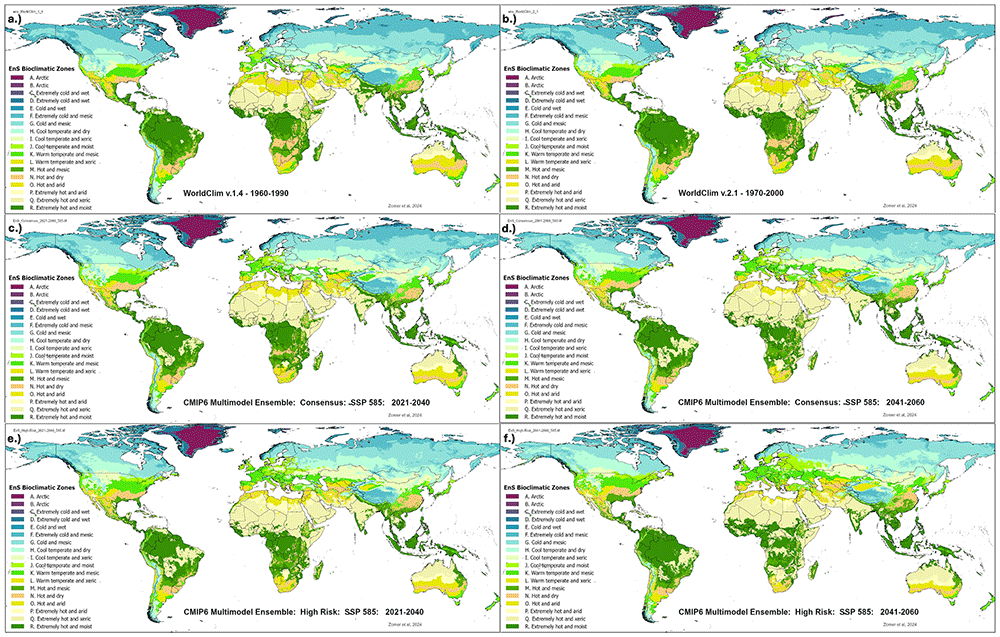
Figure 1. Future_Global_EnS_Database – historical and projected environmental stratification (EnS) datasets developed and used in the global analysis.
EnS bioclimatic stratification for two historical periods: a.) 1960–1990; b.) 1970–2000. EnS bioclimatic stratification for CMIP Phase 6 Earth System Models projections, here illustrated with examples for two future time periods for the “Consensus” and the “High Risk” Ensembles: c.) Consensus Ensemble for 2021–2040; d.) Consensus Ensemble for 2041–2060; e.) High Risk Ensemble for 2021–2040; f.) High Risk Ensemble for 2041–2060.
Methods
EnS bioclimatic stratification
A statistically derived bioclimatic stratification, which we refer to here as “EnS” to differentiate our results from the original GEnS, but based on the GEnS dataset produced by Metzger et al.10, was used to predict and understand the nature and magnitude of projected changes in the spatial distribution of bioclimatic conditions globally. The modeling approach9,48 reconstructs a high resolution global EnS bioclimatic stratification based on the statistical profiles of the original GEnS strata and zones. Both the geospatial classification of the GEnS dataset and its associated taxonomy of bioclimatic strata were used as the starting point, training dataset, and overall context for the reconstructed EnS bioclimatic stratification based on historical and projected future climatic conditions.
The EnS analysis uses the same four variables as used to derive the original GEnS, as described above, to reconstruct the global EnS, using both historical and projected future climatic datasets. To develop the reconstructed (global) EnS stratification first for the historical period of 1960–1990 and then for the 1970–2000 time period, which is used as the comparative baseline in this analysis, the four selected variables were used to develop profiles and reconstruct the EnS strata based on the original GEnS and the WorldClim v1.4 dataset (for 1960–1990) as originally used in the GEnS analysis. An iterative statistical clustering method learning technique (ISODATA)57,58 was used to stratify (cluster) the globe into 125 strata, aggregated into 18 zones, to construct this baseline EnS dataset for 1970–2000. Consistent descriptive names were attributed to strata and zones based upon the original GEnS taxonomy, with first letters (in alphabetical order) and lower numbers characterizing colder zones and strata. Statistical signature profiles were derived from the original GEnS dataset (which was based upon WorldClim 1.4) using the Maximum Likelihood Classification algorithm in ArcGIS 10.8 (ESRI).
Based on the confusion matrix comparing the original GEnS data versus the reconstructed EnS classification (for 1960–1990, i.e. WorldClim v 1.4), the overall user accuracy for the EnS bioclimatic strata was 91.7% and the Kappa Coefficient (k-Cohen) was 0.916. This compared favorably to other similar efforts59. Soteriades et al.11 compared several alternative classifiers on a similar dataset, identifying Random Forest Classifier60 as the most accurate and appropriate for their approach. However, in this case, none of the methods tested matched or exceeded the results obtained using the Maximum Likelihood Classifier using the four variables identified in the construction of the original GEnS. This was perhaps influenced by the coarser resolution of their datasets.
The signature profiles of the original GEnS strata obtained from the Maximum Likelihood Classifier were used to reconstruct the EnS stratification based first on the WorldClim v1.4 dataset, to evaluate the accuracy of the classification. Then, these were used to classify the WorldClim v2.1 dataset, to develop the EnS WC_2.1 historical baseline dataset, representing the averaged time period of 1970–2000, and then for all of the selected 22 CMIP6 ESM for each of the two time periods included in this study (2021–2040; 2041–2060). Zomer et al.9,17 outlines a detailed presentation of the EnS stratification methodology and its application to future climate projection data, as used in this study, and described below.
Modeling of projected future climate conditions
Projected impacts on bioclimatic conditions are modeled by reconstructing the global stratification based upon future climate conditions both as modeled by each individual CMIP6 ESM (n = 22) included in the study, and by two majority ensembles of ESM results61. Mora et al.62 tested the robustness of averaged ensembles based on historical observation data (1985–2005) and found a higher correlation when using multi-model averages, echoing advice provided in IPCC AR563. CMIP6 represents a significant advancement in climate modeling, incorporating more sophisticated representations of ice, water, and cloud dynamics compared to its predecessor, CMIP5. These models integrate a broader array of physical processes, reflecting ongoing efforts to enhance the realism of climate projections. However, the IPCC has acknowledged an issue of “hot” models, wherein some projections suggest considerably higher levels of equilibrium climate sensitivity (ECS), that is, higher levels of future warming. Including these into averaged ensembles creates a risk of studies reporting projections that are overly influenced by the “hot models” and inconsistent with IPCC assessed warming averages64. The IPCC’s Sixth Assessment Report (AR6)1,65 considered this and reconciled the climate models used with observational data, including global mean temperature rise, sea-level changes, and ocean heat content. Using statistical methods, the IPCC derived projections that harmonize with multiple lines of empirical evidence, producing “assessed warming” estimates. For our analysis, 22 ESM were evaluated and identified (Table 1), considering the availability of downscaled CMIP6 ESM50 and their transient climate response (TCR) rankings66,67 Based upon the distribution of average global mean annual temperature and mean annual precipitation of the 22 CIMP6 ESM within the 2021–2040 time period (Figure 2), and following the guidance provided by Hausfather et al.64 to exclude “hot models’ to approximate the IPCC AR6 averages, 15 ESM were identified to comprise a “Consensus” ensemble which explicitly excluded the hottest models (Table 1). However, as there is still more than a 5% chance for higher ECS models to predict future temperatures64, a high sensitivity subset of 5 “hot models” was identified to constitute a “High-Risk” ensemble, outlining the potential “risk space” of extreme outcomes. Recent climatic events, however, have also brought these more extreme scenarios more relevant to risk assessment68.
Table 1. Available EnS Datasets in the Future_Global_EnS_Database Used in the Global EnS Analysis.
Available datasets in the Future_Global_EnS_Database, developed and used in the global EnS analysis, including two historical datasets, 22 CMIP Phase 6 Earth System Models (ESM), calculated for each of their respective four Shared Socio-Economic Pathways (SSP: 1-2.6; 2-4.5; 3-7.0; 5-8.5), for two time periods (2021-2040; 2041-2060), and two multi-model majority ensembles (Consensus, High-Risk).
| Historical Datasets | | | ESMs included within Ensemble |
|---|
WorldClim 1.4 (1960–
1990) |
|---|
WorldClim 2.1 (1970–
2000) |
|---|
| Earth System Models (ESM) | Year: 2021–2040 | Year: 2041–2060 | MultiModel Ensemble |
|---|
| SSP Scenario: | 126 | 245 | 370 | 585 | 126 | 245 | 370 | 585 | All | Consensus | High-Risk |
|---|
| ACCESS-CM2 | X | X | X | X | X | X | X | X | X | | X |
| ACCESS-ESM1-5 | X | X | X | X | X | X | X | X | X | X | |
| CanESM5 | X | X | X | X | X | X | X | X | X | | X |
| CanESM5-CanOE | X | X | X | X | X | X | X | X | X | | X |
| CMCC-ESM2 | X | X | X | X | X | X | X | X | X | X | |
| CNRM-CM6-1 | X | X | X | X | X | X | X | X | X | X | |
| CNRM-CM6-1-HR | X | X | X | X | X | X | X | X | X | X | |
| CNRM-ESM2-1 | X | X | X | X | X | X | X | X | X | X | |
| FIO-ESM-2-0 | X | X | | X | X | X | | X | X | | |
| GFDL-ESM4 | X | | X | | X | | X | | X | | |
| GISS-E2-1-G | X | X | X | X | X | X | X | X | X | X | |
| GISS-E2-1-H | X | X | X | X | X | X | X | X | X | X | |
| HadGEM3-GC31-LL | X | X | | X | X | X | | X | X | | X |
| INM-CM4-8 | X | X | X | X | X | X | X | X | X | X | |
| INM-CM5-0 | X | X | X | X | X | X | X | X | X | X | |
| IPSL-CM6A-LR | X | X | X | X | X | X | X | X | X | X | |
| MIROC-ES2L | X | X | X | X | X | X | X | X | X | X | |
| MIROC6 | X | X | X | X | X | X | X | X | X | X | |
| MPI-ESM1-2-HR | X | X | X | X | X | X | X | X | X | X | |
| MPI-ESM1-2-LR | X | X | X | X | X | X | X | X | X | X | |
| MRI-ESM2-0 | X | X | X | X | X | X | X | X | X | X | |
| UKESM1-0-LL | X | X | X | X | X | X | X | X | X | | X |
| | | No. of ESM in Ensemble |
| Total: | 22 | 21 | 20 | 21 | 22 | 21 | 20 | 21 | 20 - 22 | 15 | 5 |
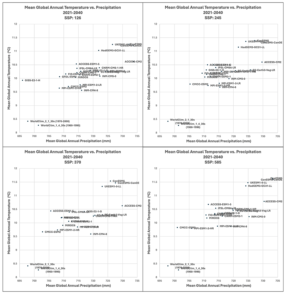
Figure 2. Distribution of 22 CMIP6 Earth System Models along temperature and precipitation gradients (2021–2040).
Distribution of average global mean annual temperature and mean annual precipitation of 22 CIMP6 ESM for four shared socio-economic pathways (SSP: 1–26; 2–45; 3–70; 5–85) for the time period 2021–2040.
Four emission scenarios, or CMIP6 Shared Socio-Economic Pathways (SSP)61,69 are analyzed for each of the 22 ESM, and for each of the two ensembles. However, to simplify the presentation of results, the SSP 5–8.5 for the two ensembles is primarily discussed in the text, with the rationale that global climate is currently worryingly close to tracking this worst-case scenario70. However, full results for all four emission scenarios are included in the extended materials, or available upon request. The downscaled ESMs (available from WorldClim.org) were downscaled using the Delta method71 to 30 arc sec resolution (equivalent to ~1 km2 at the equator) and using the WorldClim 2.1 historical dataset (1970–2000) as baseline for bias correction. The Maximum Likelihood Classification72 algorithm in ArcGIS 10.873 was used to construct the projected future spatial distribution of strata, using the modeled future climate conditions as predicted by each of the available CIMP6 ESM and SSP emission scenario combinations (n = 168) for each of the two time periods as input parameters. Selected models within each SSP were combined into a majority ensemble result, using the class with the majority of occurrence within any grid cell as the class for that location. The rate of occurrence of other classes is used as a measure of the uncertainty among models (Table 2). Average uncertainty for strata ranged from 76% to 85%, with an overall average mean uncertainty amongst all ensembles of 81.6%. In general, there was found to be a high level of agreement amongst the ESM included within each of the respective multimodel ensembles as reflected by the Coefficient of Variation of their input variables (Table 3). Agreement was relatively high at the global level for the basic parameters of annual average temperature and annual average precipitation, somewhat less for annual averaged PET and AI, slightly decreasing in the 2041–2060 time period, with significant variability across regions (Figure 3).
Table 2. Mean Percentage of Agreement Among Earth System Models (ESM) Included Within Each Ensemble.
Mean percentage of agreement among CMIP Phase 6 - Earth System Models (ESM) included within two majority ensembles (Consensus; High Risk), as a measure of uncertainty, for two time periods (2021-2040; 2041-2060), and two multi-model majority ensembles (Consensus; High-Risk).
| Mean Percentage of Agreement |
|---|
| Year | Ensemble | SSP | Average |
|---|
| | 126 | 245 | 370 | 585 | |
|---|
| 2021–2040 | Consensus | 83.15 | 83.72 | 84.20 | 82.97 | 83.51 |
| High-Risk | 85.92 | 85.23 | 83.97 | 84.75 | 84.97 |
| 2021–2040 Average | 84.54 | 84.48 | 84.09 | 83.86 | 84.24 |
| | | | | | |
| 2041–2060 | Consensus | 78.53 | 78.20 | 79.43 | 77.04 | 78.30 |
| High-Risk | 83.52 | 81.22 | 77.88 | 76.09 | 79.68 |
| 2041–2060 Average | 81.03 | 79.71 | 78.66 | 76.57 | 78.99 |
| Overall Average | 82.78 | 82.09 | 81.37 | 80.21 | 81.61 |
Table 3. Coefficient of Variation of Key Bioclimatic Variables.
Coefficient of Variation (CoV) of key variables among selected datasets within ensembles used as input to the EnS stratification analysis: annual mean temperature (tmean_yr); annual precipitation (prec_yr); annual PET (pet_yr); and Aridity Index, for two time periods (2021-2040; 2041-2060), and two multi-model majority ensembles (Consensus; High-Risk).
| Multi-model Ensemble | | Coefficient of Variation (%) |
|---|
| 2021-2040 |
|---|
| Scenario | tmean_yr | prec_yr | pet_yr | aridity_index |
|---|
| Consensus | 126 | 1.44 | 3.64 | 2.37 | 4.75 |
| 245 | 1.44 | 3.65 | 2.37 | 4.83 |
| 370 | 1.36 | 3.85 | 2.33 | 5.12 |
| 585 | 1.48 | 4.31 | 2.61 | 5.73 |
| Ensemble average: | 1.43 | 3.86 | 2.42 | 5.11 |
| High Risk | 126 | 1.09 | 2.63 | 1.71 | 3.72 |
| 245 | 1.17 | 2.68 | 1.75 | 3.80 |
| 370 | 1.30 | 2.61 | 1.69 | 3.58 |
| 585 | 1.22 | 2.88 | 1.71 | 3.91 |
| Ensemble average: | 1.20 | 2.70 | 1.72 | 3.75 |
| Multi-model Ensemble | | 2041-2060 |
|---|
| Scenario | tmean_yr | prec_yr | pet_yr | aridity_index |
|---|
| Consensus | 126 | 1.44 | 3.70 | 2.41 | 4.70 |
| 245 | 1.44 | 3.82 | 2.46 | 4.90 |
| 370 | 1.36 | 4.03 | 2.44 | 5.19 |
| 585 | 1.48 | 4.49 | 2.71 | 5.79 |
| Ensemble average: | 1.43 | 4.01 | 2.51 | 5.15 |
| High_Risk | 126 | 1.25 | 3.18 | 2.17 | 4.67 |
| 245 | 1.34 | 3.47 | 2.40 | 5.14 |
| 370 | 1.72 | 3.78 | 2.80 | 5.66 |
| 585 | 1.76 | 4.32 | 3.04 | 6.42 |
| Ensemble average: | 1.52 | 3.69 | 2.60 | 5.47 |
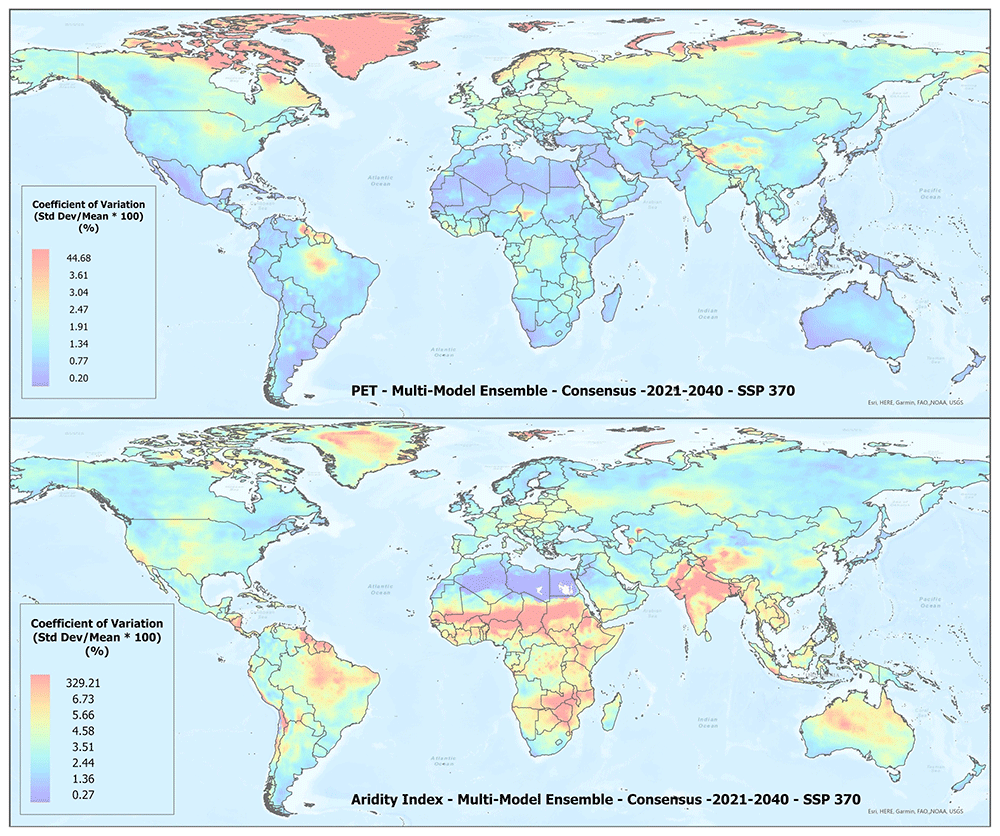
Figure 3. Example of spatial variation of Coefficient of Variation f(CoV) of PET and Aridity Index.
Coefficient of variation of PET and Aridity Index of the “Consensus” multimodel majority ensemble for the SPP 370 scenario, shown here to illustrate variation in agreement among the CMIP Phase 6 - Earth System Models (ESM) included within the respective ensemble across the various global regions.
Shifting global bioclimatic conditions
Baseline metrics
An overview of the distribution of the global average annual temperature and average annual precipitation projected by the two ensembles, as articulated for each SSP (Figure 4) illustrates that all models indicate global trends of increasing precipitation and increasing temperature in the near-term, more so by the 2041–2060 time period. However, when considering the projected global increase in PET (Figure 5), there emerges a distinct and significant drying trend indicated by decreasing AI values, both in the near-term, and again, more so by 2041–2060. There is, however, significant variability exhibited among regions (Figure 3).
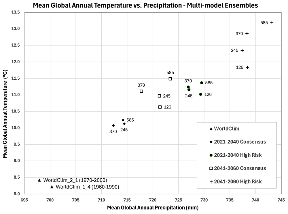
Figure 4. Distribution of historical and projected global averaged annual temperature and annual precipitation.
Distribution of historical and projected global averaged annual temperature (°C) and annual precipitation (mm) of two averaged multi-model ensembles, across four shared socio-economic pathways (SSP: 1–26; 2–45; 3–70; 5–85).
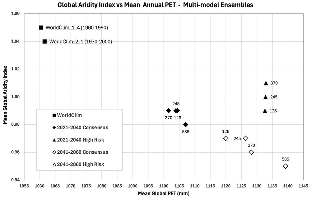
Figure 5. Distribution of historical and projected global averaged PET and Aridity Index.
Distribution of historical and projected global averaged PET (mm) and the aridity index (AI) of two averaged multi-model ensembles, across four shared socio-economic pathways (SSP: 1–2.6; 2–4.5; 3–7.0; 5–8.5). Higher AI values indicate wetter conditions, lower values indicate drier conditions.
Basic characteristics and key metrics of the 18 EnS Zones, including parameters used in the analysis, are described in Table 4, including their areal distribution, average elevation, several temperature and precipitation metrics, average annual potential evapotranspiration (PET) and aridity index. Cold and Arctic Zones (A-G) generally have lower temperatures, higher elevations, and more significant precipitation in some cases. Likewise, they generally have very high aridity indices, indicating they are less arid, sometimes wet, but this is confounded by many months of temperature below freezing so that PET and plant available moisture are less interpretable, or relevant. Temperate Zones (H-L) have moderate temperatures with varying levels of moisture. The aridity indices here are generally moderate to saturated (1.0) or above, indicating these zones are relatively more humid or mesic (moderately wet). Dry, Arid and Xeric Zones (L,N-Q) are the most arid, characterized by higher temperatures, lower precipitation, higher potential evapotranspiration and low AI values. In general, zones like Extremely Hot and Arid (P) and Extremely Hot and Xeric (Q) are expected to have very dry conditions, while Arctic and Cold zones have lower temperatures and can be both dry or wet.
Table 4. Historical Characteristics of Global EnS Bioclimatic Zones.
Historical characteristics of global EnS bioclimatic zones, as per the 1970-2000 (WorldClim v2.1) baseline, including Total Area (km2), Average Elevation (m asl), Mean (tmean_yr), Minimum (tmin_yr), and Maximum (tmax_yr) Annual Temperature (°C), Standard Deviation of the Mean Annual Temperature (tmean_sd ; °C), Annual Precipitation (prec_yr; mm), Potential Evapotranspiration (PET; mm), Standard Deviation of the PET (pet_sd; mm), and the Aridity Index.
Dataset:
WorldClim
2.1 | Area | Elev | tmean_
yr | tmean_
sd | tmin_
yr | tmax_
yr | tmean_dd | prec_
yr | pet_
yr | pet_
sd | Aridity
Index |
|---|
EnS Zones:
1970–2000 | km2 | m asl | °C | mm |
|---|
| A. Arctic | 1,395,834 | 2,406 | -21.01 | 9.09 | -24.12 | -17.90 | 0 | 625 | 76 | 9 | 9.86 |
| B. Arctic | 3,107 | 2,221 | -9.80 | 5.99 | -13.22 | -6.37 | 6 | 1516 | 202 | 18 | 7.51 |
C. Extremely
cold and wet | 201,175 | 1,408 | -8.54 | 6.49 | -11.42 | -5.66 | 548 | 1506 | 228 | 17 | 5.96 |
D. Extremely
cold and wet | 1,087,896 | 857 | -15.34 | 10.79 | -18.31 | -12.36 | 124 | 295 | 148 | 16 | 2.08 |
E. Cold and
wet | 959,683 | 816 | 1.45 | 5.54 | -1.85 | 4.75 | 1388 | 1576 | 441 | 29 | 3.56 |
F. Extremely
cold and
mesic | 15,175,626 | 1,169 | -9.08 | 13.24 | -13.60 | -4.55 | 889 | 375 | 375 | 35 | 1.02 |
G. Cold and
mesic | 16,925,555 | 695 | -1.24 | 12.41 | -6.70 | 4.22 | 1900 | 539 | 617 | 48 | 0.87 |
H. Cool
temperate
and dry | 10,134,182 | 888 | 4.78 | 10.78 | -1.19 | 10.76 | 2868 | 426 | 859 | 55 | 0.51 |
I. Cool
temperate
and xeric | 6,729,294 | 770 | 9.30 | 10.83 | 2.87 | 15.72 | 3953 | 270 | 1080 | 63 | 0.26 |
J. Cool
temperate
and moist | 2,827,167 | 574 | 9.72 | 6.46 | 5.00 | 14.43 | 3651 | 1101 | 873 | 44 | 1.30 |
K. Warm
temperate
and mesic | 8,084,307 | 822 | 14.20 | 6.46 | 8.42 | 19.98 | 5205 | 931 | 1199 | 46 | 0.80 |
L. Warm
temperate
and xeric | 5,476,129 | 728 | 16.92 | 6.04 | 9.88 | 23.97 | 6180 | 374 | 1462 | 54 | 0.26 |
M. Hot and
mesic | 9,861,417 | 681 | 22.62 | 2.41 | 16.81 | 28.43 | 8254 | 1337 | 1623 | 24 | 0.87 |
N. Hot and
dry | 10,386,019 | 753 | 19.51 | 4.55 | 13.10 | 25.91 | 7120 | 834 | 1538 | 39 | 0.57 |
O. Hot and
arid | 5,840,002 | 462 | 22.41 | 6.85 | 15.04 | 29.77 | 8185 | 112 | 1781 | 56 | 0.06 |
P. Extremely
hot and arid | 4,675,742 | 455 | 25.06 | 6.22 | 17.67 | 32.45 | 9155 | 172 | 1923 | 50 | 0.09 |
Q. Extremely
hot and xeric | 14,623,764 | 292 | 27.58 | 3.64 | 20.85 | 34.31 | 10071 | 494 | 1977 | 31 | 0.26 |
R. Extremely
hot and
moist | 19,976,113 | 283 | 25.56 | 1.17 | 20.38 | 30.75 | 9330 | 1860 | 1685 | 16 | 1.12 |
Shifting areal distribution of bioclimatic zones under climate change scenarios
The areal distribution of the EnS zones is given in Table 5 and Figure 6, reflecting the spatial extent of different homogenous bioclimatic zones across the globe during the baseline period of 1970–2000. Among the large zones, the Extremely Hot and Moist zone has the largest area, covering nearly 20 million km2, with Extremely Cold and Mesic (F) covering more than15 million km2 and the Cold and Mesic (G) almost 17 million km2. The Cool Temperate and Dry (H) zone, covering over 10 million km2, represents areas with cooler climates but limited precipitation. Warm Temperate and Mesic (K) and Cool Temperate and Moist (H) zones, with areas of 8 million km2 and 2.8 million km2 respectively, typify temperate regions with conducive temperature and moisture conditions. It represents a significant portion of the Earth’s populated surface, generally signifying regions with moderate temperatures and sufficient moisture for vegetation and agricultural production. By comparison, Hot and Extremely Hot regions cover vast areas of the globe, with over 14 million km2 of Extremely Hot and Xeric (Q) conditions, more than 10 million km2 of Hot and Dry (N), and nearly 10 million km2 of Hot and Arid (O). The Hot and Dry/Arid zones are typically found in desert regions, while the Extremely Hot and Moist (R) zone, covering nearly 20 million km2, is common in tropical rainforests biomes. Extremely Hot and Arid (P) covers a substantial area of over 4 million km2, primarily in deserts and other dry regions. Arctic (A/B) zones, with about 1.4 million km2 combined, are much smaller, reflecting the limited extent of these frigid regions which are generally limited to polar regions and high elevations.
Table 5. Historical Area of EnS Bioclimatic Zones and Percent Change for Two Future Time Periods.
Total area of EnS bioclimatic zones (km2) globally for one historical time period (1970-2000) and Percent Change (%) in Total Area for two future projected time periods (2021-2040; 2041-2060), evaluated across four Shared Socio-Economic Pathways (SSP: 1-2.6; 2-4.5; 3-7.0; 5-8.5).
| Global Area - EnS Zones (% change) | 1970–2000 | 2021–2040 | 2041–2060 |
|---|
| Model | SSP: | WC_2.1 | 126 | 245 | 370 | 585 | 126 | 245 | 370 | 585 |
|---|
| Consensus | Arctic | 1,395,834 | (3) | (4) | (3) | (4) | (5) | (6) | (6) | (7) |
| Arctic | 3,107 | 64 | 85 | 76 | 73 | 73 | 82 | 93 | 105 |
| Extremely cold and wet | 201,175 | 10 | 12 | 11 | 15 | 18 | 25 | 24 | 30 |
| Extremely cold and wet | 1,087,896 | (24) | (23) | (21) | (24) | (29) | (32) | (33) | (38) |
| Cold and wet | 959,683 | (7) | (7) | (6) | (8) | (8) | (9) | (10) | (10) |
| Extremely cold and mesic | 15,175,626 | (25) | (25) | (23) | (27) | (33) | (38) | (38) | (45) |
| Cold and mesic | 16,925,555 | (2) | (3) | (2) | (3) | (3) | (3) | (3) | (3) |
| Cool temperate and dry | 10,134,182 | (1) | (0) | (2) | 0 | (1) | (0) | (2) | (2) |
| Cool temperate and xeric | 6,729,294 | 14 | 14 | 13 | 15 | 16 | 17 | 18 | 21 |
| Cool temperate and moist | 2,827,167 | 8 | 9 | 9 | 9 | 10 | 11 | 10 | 9 |
| Warm temperate and mesic | 8,084,307 | 7 | 7 | 6 | 8 | 10 | 11 | 12 | 14 |
| Warm temperate and xeric | 5,476,129 | (9) | (9) | (10) | (11) | (13) | (17) | (17) | (17) |
| Hot and mesic | 9,861,417 | (14) | (14) | (14) | (16) | (18) | (20) | (22) | (24) |
| Hot and dry | 10,386,019 | (14) | (14) | (15) | (15) | (16) | (19) | (20) | (22) |
| Hot and arid | 5,840,002 | (15) | (14) | (15) | (17) | (20) | (24) | (26) | (31) |
| Extremely hot and arid | 4,675,742 | 10 | 11 | 12 | 11 | 13 | 14 | 12 | 10 |
| Extremely hot and xeric | 14,623,764 | 44 | 45 | 44 | 49 | 59 | 69 | 75 | 83 |
| Extremely hot and moist | 19,976,113 | 2 | 2 | 2 | 2 | 1 | 1 | (0) | 1 |
| High-Risk | Arctic | 1,395,834 | (9) | (9) | (8) | (10) | (12) | (18) | (21) | (22) |
| Arctic | 3,107 | 302 | 405 | 481 | 395 | 345 | 514 | 973 | 841 |
| Extremely cold and wet | 201,175 | 22 | 24 | 37 | 30 | 35 | 55 | 96 | 88 |
| Extremely cold and wet | 1,087,896 | (33) | (35) | (34) | (36) | (38) | (36) | (40) | (43) |
| Cold and wet | 959,683 | (7) | (7) | (5) | (8) | (12) | (16) | (16) | (23) |
| Extremely cold and mesic | 15,175,626 | (46) | (46) | (48) | (50) | (55) | (60) | (66) | (69) |
| Cold and mesic | 16,925,555 | 2 | 1 | (1) | 0 | 2 | (2) | (8) | (11) |
| Cool temperate and dry | 10,134,182 | (2) | (1) | (1) | (2) | (7) | (6) | (3) | (0) |
| Cool temperate and xeric | 6,729,294 | 16 | 17 | 20 | 19 | 17 | 14 | 7 | 2 |
| Cool temperate and moist | 2,827,167 | 25 | 23 | 26 | 24 | 28 | 39 | 51 | 60 |
| Warm temperate and mesic | 8,084,307 | 15 | 16 | 17 | 17 | 22 | 26 | 34 | 34 |
| Warm temperate and xeric | 5,476,129 | (12) | (14) | (12) | (12) | (14) | (13) | (13) | (10) |
| Hot and mesic | 9,861,417 | (19) | (19) | (18) | (19) | (23) | (25) | (25) | (27) |
| Hot and dry | 10,386,019 | (17) | (18) | (18) | (18) | (21) | (23) | (25) | (27) |
| Hot and arid | 5,840,002 | (24) | (25) | (26) | (27) | (30) | (35) | (39) | (42) |
| Extremely hot and arid | 4,675,742 | 10 | 12 | 11 | 11 | 10 | 5 | (2) | (5) |
| Extremely hot and xeric | 14,623,764 | 68 | 70 | 66 | 72 | 79 | 86 | 84 | 86 |
| Extremely hot and moist | 19,976,113 | (1) | (1) | 2 | 1 | 4 | 8 | 19 | 25 |
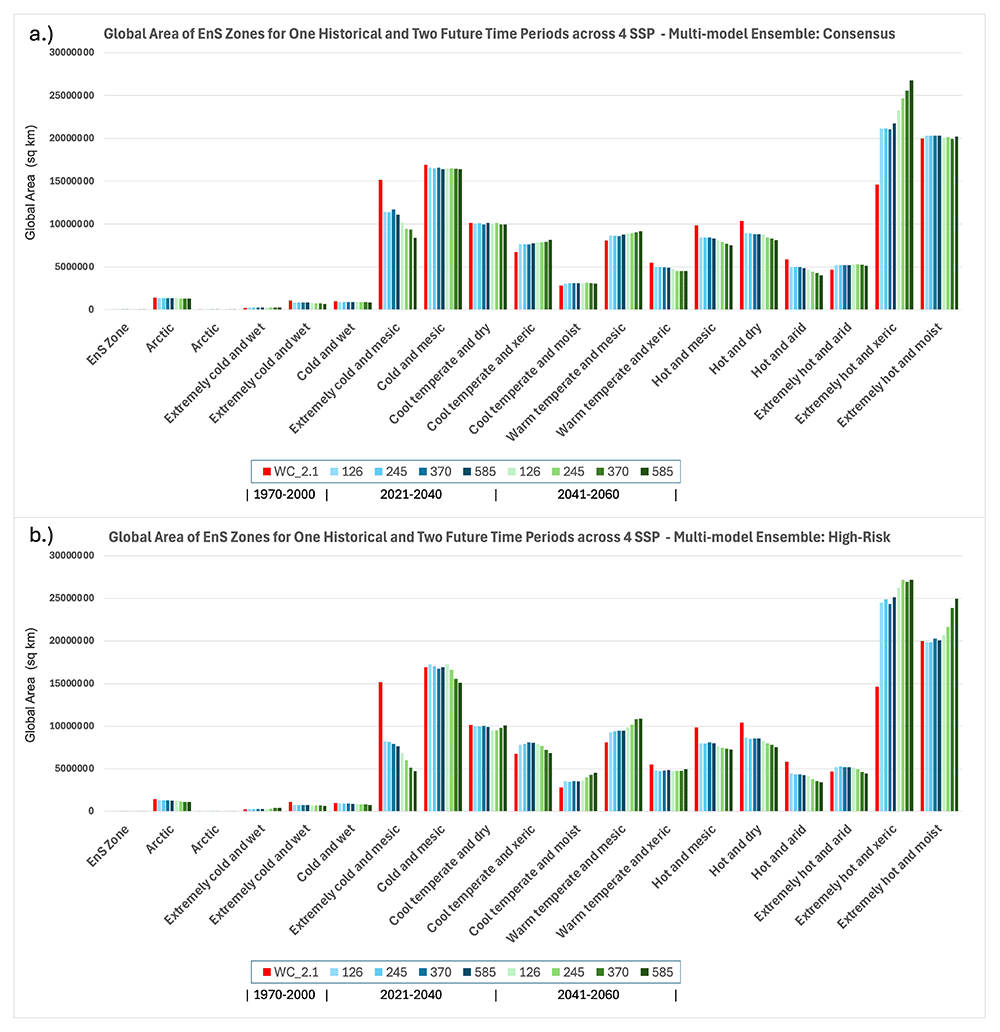
Figure 6. Global Area of Ens Zones for One Historical and Two Future Time Periods.
Global area (km2) of Ens bioclimatic zones for one historical (Baseline: WC_2.1: 1970-2000) and two future time periods (2021–2040; 2041–2060) showing results for two multi-model majority ensembles: a.) Consensus and b.) High-Risk.
Below, as an illustrative example, we provide a summary of key findings reporting the absolute areal changes and percent change for each of the EnS Zones with a comparison from the baseline period (1970–2000) to mid-Century (2041–2060) for both the Consensus and the High-Risk scenarios, as projected under the SSP5 8.5 scenario (full results for all SSPs are given in Table 5).
Summary of projected bioclimatic zone shifts under SSP5–8.5 by mid-century
Projected changes in bioclimatic zone extent under the high-emissions SSP5–8.5 scenario (2041–2060) relative to the historical baseline (1970–2000) reveal substantial spatial redistribution of climatic envelopes. These changes reflect both thermal and hydrological reorganizations of the terrestrial climate space. Below, we summarize each EnS zone’s shift in area.
• Arctic (A): This zone represents the coldest and most climatically stable Arctic regions, typically underlain by continuous permafrost. Area is projected to decline from 1,395,834 km2 to 1,301,659 km2 under the Consensus model (−6.7%), and to 1,088,848 km2 under the High-Risk model (−22.0%).The reduction is consistent with observed permafrost degradation and earlier snowmelt at high latitudes.
• Arctic (B): A transitional Arctic zone, typically featuring discontinuous permafrost and tundra-shrub ecotones. Although comprising a relatively very small areal extent, this is projected to expand from 3,107 km2 to 6,358 km2 under the Consensus model (+104.6%), and to 29,225 km2 under the High-Risk model (+840.6%). This dramatic expansion reflects shrub encroachment, and warming-induced northward shifts of boreal ecosystems, and highlights this zone as a sensitive early indicator of Arctic climate response.
• Extremely Cold and Wet (C): Found in polar and alpine areas with persistent cold, high precipitation and prolonged snow cover. Area increases from 201,175 km2 to 261,985 km2 (+30.2% Consensus) and to 377,385 km2 (+87.6% High-Risk). Some of these gains may result from upward migration of cold-wet regimes into formerly drier, slightly colder uplands.
• Extremely Cold and Wet (D): This zone comprises persistent cold-wet conditions, often found in high montane, glacial margins, or snow-dominated regions with extended snow cover and short growing seasons. Declines from 1,087,896 km2 to 676,593 km2 (−37.8% Consensus) and to 619,463 km2 (−43.1% High-Risk). These reductions are consistent with warming-induced snowline retreat, decreasing snowpack persistence, and reduced cold-season moisture retention.
• Cold and Wet (E): Encompasses boreal forests and peat-rich landscapes with long winters and moderate precipitation. Area declines from 959,683 km2 to 860,979 km2 (−10.3% Consensus), and to 742,905 km2 (−22.6% High-Risk). The contraction of areal extent is likely indicative of warming-induced transitions to more mesic or temperate classifications, and aligns with observed boreal forest stress and increasing fire activity across high latitudes.
• Extremely Cold and Mesic (F): Comprising dry, cold steppe tundra, and northern boreal / tundra margins with limited precipitation and extended frost periods. Contracts from 15,175,626 km2 to 8,392,612 km2 (−44.7% Consensus) and to 4,691,945 km2 (−69.1% High-Risk). This is a highly impacted zone, reflecting widespread loss of cold continental interiors and high climate sensitivity.
• Cold and Mesic (G): Typical of mid-latitude mixed forests and highland temperate grassland, encompassing much of the temperate coniferous belt. such as the northern Rockies, central Asia, and the southern Andes. These systems are climatically transitional, often positioned between boreal and temperate zones, and support a mix of forest types, grazing lands, and temperate biodiversity hotspots. Declines modestly from 16,925,555 km2 to 16,424,216 km2 (−3.0% Consensus), and more strongly to 15,066,298 km2 (−11.0% High-Risk), suggesting encroachment by warmer and drier conditions, potentially leading to increased vulnerability to fire, pests, and seasonal water stress.
• Cool Temperate and Dry (H): Comprised of temperate steppe, semi-arid highland, and includes dry to mesic temperate landscapes with seasonal droughts such as Eurasian steppe zones, Patagonian plains, and semi-arid highland plateaus. Area declines slightly from 10,134,182 km2 to 9,934,801 km2 (−2.0% Consensus) and to 10,102,559 km2 (−0.3% High-Risk). These relatively small shifts suggest near-term climatic stability in many of these continental interiors, but they may mask important and growing exposure to climate extremes, including shifting rainfall patterns and rising temperatures.
• Cool Temperate and Xeric (I): Comprised of temperate regions subject to drought and high inter-seasonal variability, low and erratic rainfall, often under strong rain-shadow influence or within continental interiors — such as the Great Plains, western China, or Anatolia. These areas support grazing, irrigated agriculture, and drought-adapted ecosystems. Expands from 6,729,294 km2 to 8,165,562 km2 (+21.3% Consensus), and to 6,844,484 km2 (+1.7% High-Risk). Although substantially less under the High-Risk scenario, this increase may reflect warming-induced aridification and a thermally driven shift into more xeric classifications, with growing seasonal moisture stress and elevated evaporative demand likely to affect both ecosystem function and agricultural potential.
• Cool Temperate and Moist (J): Found in humid to sub-humid temperate regions, this zone includes parts of central and northern Europe, the southern Andes, eastern Australia, and the Pacific Northwest of North America. These landscapes support broadleaf and mixed forests and are key zones for both biodiversity and forestry. Increases from 2,827,167 km2 to 3,070,582 km2 (+8.6% Consensus), and to 4,514,481 km2 (+59.7% High-Risk). Expansion may reflect warming in currently colder zones into mesic temperate regimes and becoming more suitable for temperate forest assemblages.
• Warm Temperate and Mesic (K): Agriculturally productive regions with generally high land-use intensity, including Mediterranean climatic zones (e.g., southern Europe, California, parts of Chile and South Africa) and moist subtropical highlands (e.g., Ethiopian plateau, southern China, southeastern Brazil). These regions support mixed cropping systems, vineyards, and high-value horticulture, often with seasonal rainfall regimes. Expands from 8,084,307 km2 to 9,186,018 km2 (+13.6% Consensus), and to 10,858,638 km2 (+34.3% High-Risk). This expansion may reflect the poleward and upslope encroachment of warmer, wetter conditions into former temperate zones and drylands, potentially enhancing agricultural suitability in some areas while also increasing exposure to heatwaves, evapotranspiration losses, and seasonal climate variability.
• Warm Temperate and Xeric (L): Found in semi-arid Mediterranean and subtropical upland areas characterized by strong interannual rainfall variability and pronounced dry seasons. These regions include parts of the Middle East, southwestern North America, central Asia, and northern Mexico — areas often supporting extensive rangelands or low-input rainfed agriculture. Decreasing from 5,476,129 km2 to 4,545,379 km2 (−17.0% Consensus) and to a lesser 4,941,811 km2 (−9.8% High-Risk), which may reflect bifurcation into either wetter mesic systems (under enhanced seasonal precipitation) or into more arid and xeric classes (under warming and drying scenarios). The instability of this zone underscores its sensitivity to relatively small shifts in temperature and rainfall balance, with implications for agricultural sustainability and water stress.
• Hot and Mesic (M): Comprising tropical savannas, monsoon-influenced lowlands, and seasonally wet tropics with pronounced wet-dry cycles — including parts of India, Southeast Asia, northern South America, and sub-Saharan Africa. These areas are highly dynamic, supporting rainfed cropping systems, mixed woodlands, and fire-adapted ecosystems. Decreases from 9,861,417 km2 to 7,526,648 km2 (−23.7% Consensus), and to 7,243,885 km2 (−26.5% High-Risk). The substantial loss suggests increasing aridity and contraction of the savanna-climate envelope, with portions of this zone likely transitioning into xeric or dry forest conditions. This has critical implications for agroecological transitions, biodiversity corridors, and food security in regions dependent on monsoonal reliability. Indicative of moisture stress and encroachment of drier regimes into moist tropics.
• Hot and Dry (N): This zone spans dry subtropical belts and marginal arid environments, such as the Kalahari, Thar Desert, and interior Australia, often defined by high temperatures, erratic rainfall, and limited vegetative cover. Many of these areas lie at the climatic threshold between productive rangelands and true deserts. Declines from 10,386,019 km2 to 8,134,725 km2 (−21.7% Consensus), and to 7,542,652 km2 (−27.4% High-Risk). These reductions suggest significant ecological stress and warming-induced aridification, pushing many landscapes past thresholds for productivity or natural vegetation persistence. The contraction may also signal a trajectory into more extreme xeric or hyper-arid states, posing growing challenges for sustainable livelihoods, particularly in semi-arid agrarian zones.
• Hot and Arid (O) Typically includes interior deserts and subtropical arid zones with seasonal rainfall, such as the Sahel, Arabian Peninsula, and interior Australia. Contracts from 5,840,002 km2 to 4,020,916 km2 (−31.1% Consensus), and to 3,393,073 km2 (−41.9% High-Risk). These sharp contractions suggest many of these landscapes are exceeding the thermal and moisture thresholds defining aridity, shifting toward hyperarid conditions.
• Extremely Hot and Arid (P): This zone encompasses the world’s core desert systems — including the Sahara, the Arabian Penisula, and parts of the Iranian Plateau — characterized by extreme temperatures, minimal annual precipitation (<100 mm), and near-total absence of permanent vegetation. Expands from 4,675,742 km2 to 5,136,913 km2 (+9.9% Consensus), but slightly contracts to 4,442,277 km2 (−5.0% High-Risk). These mixed results perhaps suggest that extremely hot and hyper-arid zones may be undergoing shifts in internal characteristics and boundary definition towards novel bioclimatic conditions, with varying climate sensitivities in this hyper-arid belt.
• Extremely Hot and Xeric (Q): This zone includes dryland regions with heat and chronic moisture deficit — increasingly surpassing physiological tolerance thresholds for vegetation. It includes vast swaths of northern Africa, western Asia, interior Australia, and subtropical zones in the Americas. Areal extent of this zone expands dramatically from 14,623,764 km2 to 26,754,600 km2 (+83.0% Consensus), and to 27,194,394 km2 (+86.0% High-Risk). This consistent and extensive bioclimatic shift suggests widespread conversion of hot drylands into ultra-xeric systems with limited productivity and resilience. Such expansion has profound implications for desertification processes, biodiversity loss, climate-driven migration, and the sustainability of marginal agricultural systems under worsening aridity and heat stress.
• Extremely Hot and Moist (R): Occupying the hottest and most humid regions on Earth — including the Amazon, Congo Basin, and equatorial Southeast Asia — this zone is defined by high rainfall, persistent humidity, and high potential evapotranspiration. Area increases modestly from 19,976,113 km2 to 20,235,495 km2 (+1.3%) under the Consensus model but expands considerably to 24,941,718 km2 (+24.9%) under the High-Risk model. This projected intensification of hot-humid conditions may signal an expanded spatial extent of equatorial convection zones, with higher temperatures pushing moisture-rich regions beyond historical norms. These shifts could increase climate sensitivity in the tropics, potentially altering cloud dynamics, carbon fluxes, and biodiversity patterns — particularly in systems already close to thermal and hydrological tipping points, and imply an intensification and spatial spread of hot, humid tropical conditions.
Overall, the projections under SSP5–8.5, presented here as an illustrative high-emissions scenario, reveal a pronounced contraction of cooler and wetter bioclimatic zones, including the Arctic, extremely cold and wet, cold and wet, and cold to mesic temperate regions. These losses are especially substantial under the High-Risk ensemble. In contrast, hotter and drier zones, particularly the extremely hot and xeric class, expand dramatically, exhibiting a consistent and extensive bioclimatic shift across both ensemble models. Several transitional and agriculturally critical zones, such as warm temperate mesic areas, show notable expansion, while others (e.g., warm temperate xeric, hot and dry) are reclassified into more extreme categories. While these patterns are broadly consistent, the magnitude of change is greater under the High-Risk projections. These findings illustrate a large-scale redistribution of terrestrial climate space toward hotter and more arid regimes, underscoring the potential impacts of unmitigated climate change on ecological stability, land-use suitability, biodiversity, and the ecosystem services that underpin human well-being.
Latitudinal shifts in bioclimatic zones under climate change scenarios
Analysis of latitudinal shifts in the global EnS bioclimatic zones under future climate projections reveals a clear and measurable poleward migration of bioclimatic zones, with notable variations between hemispheres and between climate model ensembles. Mountain regions were excluded from the analysis, based upon the UNEP-WCMC Mountains of the World74 dataset, to isolate latitudinal effects from confounding elevational influences, with results clearly demonstrating that climate-driven changes in temperature and precipitation regimes are progressively altering the latitudinal distribution of bioclimatic conditions and terrestrial ecosystems.
In the Northern Hemisphere, bioclimatic zones exhibit a strong and consistent northward shift, with both the Consensus and High-Risk ensembles projecting significant poleward movement (Table 6). The Consensus model found an average latitudinal displacement of +2.75° by 2041–2060, while the High-Risk model estimates a more pronounced shift of +4.96°, with some zones migrating more than +10°. These changes are particularly evident in boreal and temperate biomes, where zones that historically averaged around 55°N now shift toward or beyond 57–60°N. This result is consistent with recent observation75, and aligns with well-documented ecological shifts in boreal and temperate biomes, where warming temperatures are enabling the expansion of temperate vegetation into traditionally boreal zones. Boreal and tundra ecosystems in Alaska, Siberia, and Fennoscandia are among the fastest-shifting systems, consistent with arctic amplification and rapid warming in these high-latitude continental interiors. These findings are consistent with the observed latitudinal changes in boreal zones75,76, as observed across Canada, Scandinavia, and northern Eurasia, where satellite data and long-term ecological monitoring indicate northward expansion of temperate vegetation and declines in boreal forest density at their southern margins. supporting evidence of a climate-induced northward migration of these ecosystems77,78. Analysis of nearly four decades of satellite data and environmental records reveal that much of the boreal forest has become greener along its northern margins and browner along its southern margins75.
Table 6. Average Latitude of Ens Bioclimatic Zones and Change for Two Future Projected Time Periods.
Average latitude of EnS bioclimatic zones (decimal degrees; geographic projection) for one historical time period (1970-2000) and change in average latitude (decimal degrees) for two future projected time periods (2021-2040; 2041-2060), a across the four Shared Socioeconomic Pathways (SSP 1-2.6; 2-4.5; 3-7.0; 5-8.5).
| Average Latitude - EnS Zones (Decimal Degrees) | Change: Decimal Degrees |
|---|
| Mountain Regions Excluded | 1970–2000 | 2021–2040 | 2041–2060 |
|---|
| Ensemble | Northern Hemisphere SSP: | WC_2.1 | 126 | 245 | 370 | 585 | 126 | 245 | 370 | 585 |
|---|
| Consensus | A. Arctic | 74.10 | 0.67 | 0.71 | 0.66 | 0.76 | 0.86 | 0.99 | 0.95 | 1.12 |
| B. Arctic | 64.06 | (0.46) | 0.07 | 0.22 | (0.30) | (0.53) | (0.65) | (0.92) | (0.90) |
| C. Extremely cold and wet | 66.47 | (2.33) | (2.22) | (2.36) | (2.25) | (2.13) | (1.91) | (1.83) | (1.67) |
| D. Extremely cold and wet | 74.73 | 0.60 | 0.55 | 0.55 | 0.54 | 0.55 | 0.61 | 0.60 | 0.60 |
| E. Cold and wet | 58.52 | 2.28 | 2.30 | 2.17 | 2.39 | 2.90 | 3.13 | 3.27 | 3.56 |
| F. Extremely cold and mesic | 65.83 | 1.27 | 1.28 | 1.14 | 1.32 | 1.77 | 2.15 | 2.07 | 2.69 |
| G. Cold and mesic | 57.04 | 2.28 | 2.30 | 2.12 | 2.48 | 2.94 | 3.25 | 3.33 | 3.78 |
| H. Cool temperate and dry | 48.72 | 3.05 | 3.08 | 2.80 | 3.37 | 4.00 | 4.54 | 4.61 | 5.29 |
| I. Cool temperate and xeric | 43.46 | 1.84 | 1.85 | 1.76 | 2.04 | 2.41 | 2.69 | 2.86 | 3.26 |
| J. Cool temperate and moist | 45.63 | 2.25 | 2.35 | 2.22 | 2.43 | 2.72 | 3.09 | 3.19 | 3.67 |
| K. Warm temperate and mesic | 36.87 | 3.15 | 3.15 | 2.87 | 3.34 | 3.99 | 4.37 | 4.56 | 5.20 |
| L. Warm temperate and xeric | 34.16 | 2.52 | 2.51 | 2.45 | 2.69 | 3.24 | 3.65 | 3.89 | 4.40 |
| M. Hot and mesic | 17.21 | 4.35 | 4.32 | 4.30 | 4.60 | 5.56 | 6.30 | 6.56 | 7.37 |
| N. Hot and dry | 29.21 | 2.03 | 2.02 | 1.87 | 2.15 | 2.55 | 2.86 | 2.97 | 3.43 |
| O. Hot and arid | 27.78 | 1.97 | 1.96 | 1.90 | 2.11 | 2.37 | 2.64 | 2.83 | 3.25 |
| P. Extremely hot and arid | 24.23 | 2.30 | 2.30 | 2.23 | 2.46 | 2.82 | 3.19 | 3.40 | 3.88 |
| Q. Extremely hot and xeric | 15.76 | 0.94 | 0.93 | 0.85 | 1.03 | 1.37 | 1.56 | 1.61 | 2.01 |
| R. Extremely hot and moist | 8.90 | (1.10) | (1.05) | (0.94) | (1.16) | (1.48) | (1.49) | (1.49) | (1.37) |
| High-Risk | A. Arctic | 74.10 | 0.44 | 0.50 | 0.86 | 0.55 | 0.61 | 0.75 | 1.72 | 1.27 |
| B. Arctic | 64.06 | 1.22 | 1.20 | 1.78 | 1.04 | 1.24 | 1.85 | 2.32 | 2.06 |
| C. Extremely cold and wet | 66.47 | (0.26) | (0.42) | (0.48) | 0.18 | (0.23) | 0.47 | 0.76 | 1.47 |
| D. Extremely cold and wet | 74.73 | 1.37 | 1.34 | 1.28 | 1.38 | 1.48 | 1.75 | 1.89 | 1.92 |
| E. Cold and wet | 58.52 | 4.46 | 4.46 | 4.62 | 4.60 | 4.98 | 5.14 | 5.12 | 5.43 |
| F. Extremely cold and mesic | 65.83 | 3.20 | 3.21 | 3.32 | 3.45 | 4.24 | 4.68 | 5.10 | 5.53 |
| G. Cold and mesic | 57.04 | 3.77 | 3.87 | 4.05 | 4.17 | 4.44 | 5.01 | 5.72 | 6.25 |
| H. Cool temperate and dry | 48.72 | 4.65 | 4.83 | 4.96 | 5.28 | 5.70 | 6.42 | 7.29 | 7.96 |
| I. Cool temperate and xeric | 43.46 | 2.82 | 2.87 | 3.03 | 3.16 | 3.54 | 3.80 | 4.23 | 4.75 |
| J. Cool temperate and moist | 45.63 | 3.66 | 3.89 | 4.19 | 4.37 | 4.90 | 5.96 | 6.75 | 7.15 |
| K. Warm temperate and mesic | 36.87 | 4.69 | 4.89 | 4.95 | 5.32 | 5.94 | 6.78 | 7.70 | 8.08 |
| L. Warm temperate and xeric | 34.16 | 3.55 | 3.71 | 3.74 | 3.98 | 4.37 | 4.93 | 5.64 | 6.03 |
| M. Hot and mesic | 17.21 | 5.99 | 6.40 | 6.21 | 6.60 | 7.57 | 8.71 | 9.53 | 10.45 |
| N. Hot and dry | 29.21 | 2.99 | 3.12 | 3.06 | 3.34 | 3.86 | 4.48 | 5.34 | 5.87 |
| O. Hot and arid | 27.78 | 2.58 | 2.68 | 2.63 | 2.85 | 3.28 | 3.79 | 4.54 | 5.36 |
| P. Extremely hot and arid | 24.23 | 3.21 | 3.23 | 3.27 | 3.42 | 3.82 | 4.37 | 5.04 | 5.35 |
| Q. Extremely hot and xeric | 15.76 | 1.54 | 1.57 | 1.63 | 1.72 | 2.15 | 2.60 | 3.42 | 3.72 |
| R. Extremely hot and moist | 8.90 | (1.55) | (1.48) | (1.30) | (1.39) | (1.14) | (0.64) | 0.21 | 0.55 |
| Ensemble | Southern Hemisphere SSP: | WC_2.1 | 126 | 245 | 370 | 585 | 126 | 245 | 370 | 585 |
|---|
| Consensus | A. Arctic | | | | | | | | | |
| B. Arctic | | | | | | | | | |
| C. Extremely cold and wet | 49.95 | (0.01) | (0.00) | (0.00) | (0.02) | (0.03) | (0.08) | (0.10) | (0.11) |
| D. Extremely cold and wet | 51.50 | 0.18 | 0.13 | 0.27 | 0.18 | 0.28 | 0.38 | 0.27 | 0.49 |
| E. Cold and wet | 48.81 | 0.62 | 0.65 | 0.75 | 0.63 | 0.79 | 0.96 | 1.17 | 1.37 |
| F. Extremely cold and mesic | 52.25 | 0.02 | 0.02 | 0.02 | 0.02 | 0.03 | 0.19 | 0.06 | (0.07) |
| G. Cold and mesic | 51.35 | 0.53 | 0.56 | 0.58 | 0.59 | 0.61 | 0.75 | 0.81 | 0.84 |
| H. Cool temperate and dry | 46.14 | 0.65 | 0.72 | 0.74 | 0.82 | 0.88 | 1.42 | 1.67 | 1.93 |
| I. Cool temperate and xeric | 43.14 | 1.51 | 1.63 | 1.66 | 1.71 | 1.87 | 2.13 | 2.18 | 2.25 |
| J. Cool temperate and moist | 42.11 | 0.85 | 0.88 | 0.94 | 0.93 | 1.09 | 1.33 | 1.49 | 1.77 |
| K. Warm temperate and mesic | 34.32 | 1.70 | 1.72 | 1.76 | 1.91 | 2.38 | 3.06 | 3.35 | 3.70 |
| L. Warm temperate and xeric | 32.01 | 1.27 | 1.34 | 1.35 | 1.46 | 1.69 | 2.12 | 2.32 | 2.60 |
| M. Hot and mesic | 16.25 | 1.50 | 1.50 | 1.48 | 1.67 | 2.07 | 2.44 | 2.63 | 2.85 |
| N. Hot and dry | 22.57 | 2.59 | 2.62 | 2.60 | 2.92 | 3.45 | 5.00 | 5.46 | 6.47 |
| O. Hot and arid | 25.95 | 1.23 | 1.31 | 1.40 | 1.41 | 1.64 | 2.13 | 2.18 | 2.40 |
| P. Extremely hot and arid | 21.80 | 1.30 | 1.49 | 1.53 | 1.57 | 1.82 | 2.26 | 2.40 | 2.52 |
| Q. Extremely hot and xeric | 14.38 | (0.13) | (0.09) | (0.07) | (0.09) | (0.15) | (0.18) | (0.32) | (0.16) |
| R. Extremely hot and moist | 8.15 | 0.60 | 0.59 | 0.62 | 0.66 | 0.65 | 0.79 | 0.93 | 0.99 |
| High-Risk | A. Arctic | | | | | | | | | |
| B. Arctic | | | | | | | | | |
| C. Extremely cold and wet | 49.95 | (0.09) | (0.08) | (0.09) | (0.08) | (0.18) | (0.24) | (0.29) | (0.37) |
| D. Extremely cold and wet | 51.50 | 0.31 | 0.38 | 0.42 | 0.24 | 0.42 | 0.71 | 1.07 | 1.16 |
| E. Cold and wet | 48.81 | 1.07 | 1.13 | 1.30 | 1.28 | 1.38 | 1.99 | 2.41 | 2.60 |
| F. Extremely cold and mesic | 52.25 | 0.11 | 0.13 | 0.11 | 0.11 | 0.06 | 0.25 | 0.23 | 0.23 |
| G. Cold and mesic | 51.35 | 0.78 | 0.80 | 0.82 | 0.83 | 0.89 | 1.01 | 1.12 | 1.17 |
| H. Cool temperate and dry | 46.14 | 1.39 | 1.43 | 1.47 | 1.59 | 2.01 | 2.80 | 3.28 | 3.57 |
| I. Cool temperate and xeric | 43.14 | 2.21 | 2.32 | 2.36 | 2.39 | 2.43 | 2.44 | 2.49 | 2.49 |
| J. Cool temperate and moist | 42.11 | 1.43 | 1.53 | 1.59 | 1.66 | 2.07 | 2.89 | 3.70 | 4.17 |
| K. Warm temperate and mesic | 34.32 | 2.99 | 3.15 | 3.16 | 3.35 | 3.95 | 4.69 | 5.25 | 5.83 |
| L. Warm temperate and xeric | 32.01 | 1.83 | 2.00 | 1.99 | 2.07 | 2.47 | 3.18 | 3.89 | 4.32 |
| M. Hot and mesic | 16.25 | 2.36 | 2.46 | 2.46 | 2.47 | 2.90 | 3.65 | 4.17 | 5.07 |
| N. Hot and dry | 22.57 | 4.23 | 4.51 | 4.43 | 4.93 | 6.22 | 7.08 | 7.75 | 8.24 |
| O. Hot and arid | 25.95 | 1.78 | 1.88 | 1.85 | 1.91 | 2.18 | 2.75 | 3.33 | 3.69 |
| P. Extremely hot and arid | 21.80 | 1.94 | 2.06 | 2.02 | 2.09 | 2.33 | 2.64 | 3.43 | 3.84 |
| Q. Extremely hot and xeric | 14.38 | (0.56) | (0.57) | (0.58) | (0.54) | (0.27) | 0.22 | 0.99 | 1.29 |
| R. Extremely hot and moist | 8.15 | 0.81 | 0.89 | 0.95 | 1.00 | 1.03 | 1.16 | 1.35 | 1.55 |
Similarly, in the Southern Hemisphere, bioclimatic zones are shifting poleward, however, at a more moderate rate compared to the Northern Hemisphere, with the Consensus model averaging +1.66°, and the High-Risk model showing a larger shift of +3.05° southward (Table 6). At least part of this asymmetry in latitudinal migration may be attributed to the greater oceanic influence in the Southern Hemisphere, which moderates temperature fluctuations. Zones typically associated with subtropical drylands and Mediterranean-type ecosystems—such as parts of southern Africa, Australia, and South America—are among those showing moderate to high latitudinal shifts globally. Bioclimatic zones typically associated with subtropical savanna and grassland systems are projected to undergo substantial latitudinal shifts—ranging up to 6–8° under high-emissions scenarios—suggesting significant ecological displacement with profound ecological and socioeconomic implications.
The asymmetry in poleward movement between hemispheres is further highlighted by the distribution of shifts across zones, as illustrated by the violin graph in Figure 7 showing a greater spread in the Northern Hemisphere’s latitudinal migration, with some zones exhibiting much faster poleward movement than others. A wider spread at higher latitudes, indicates greater variability in poleward shifts among the different bioclimatic zones, while some zones have a long tail extending farther north, suggesting that certain ecosystems (e.g., boreal forests or tundra) are shifting more rapidly. This difference suggests that regional climate variability is influencing the velocity of bioclimatic shifting, while showing that most zones are exhibiting a steady poleward movement79,80. The more constrained latitudinal shifts shown for the Southern Hemisphere reinforce the idea of a moderated response due to oceanic influence. However, certain outliers (long tails) indicate that some specific biomes, such as subtropical drylands or Mediterranean ecosystems, could shift more than others. The uneven distribution of latitudinal shifts in both hemispheres highlight the importance of regional and localized adaptation strategies to account for differential rates of climate-driven ecological change
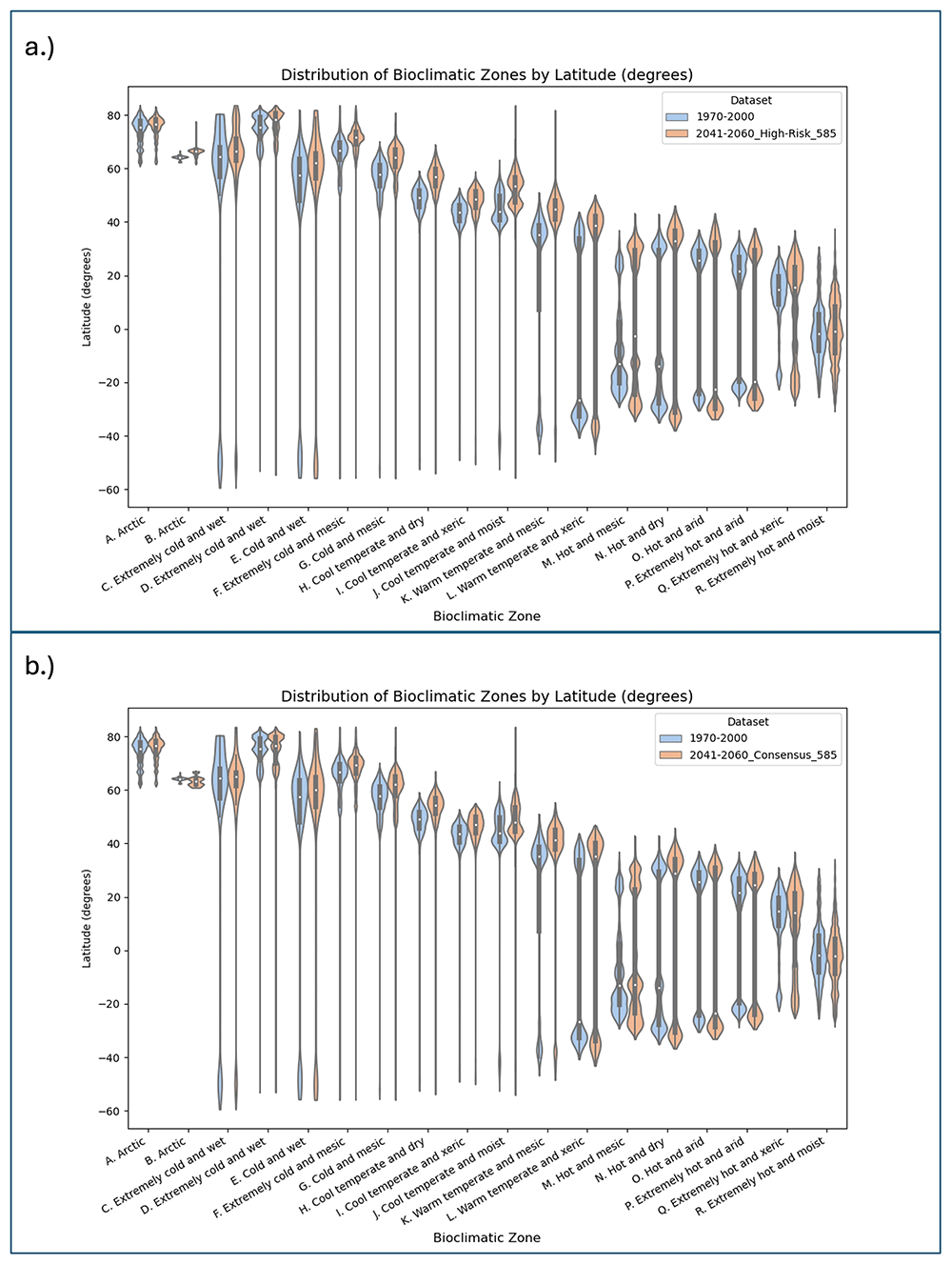
Figure 7. Distribution of EnS Bioclimatic Zones by Latitude.
Distribution of EnS bioclimatic zones by latitude (geographic degrees) comparing the historical baseline (WC_2.1; 1970–2000) with the projections for 2041–2060, evaluated for the SSP 5-8.5 scenario for both the a.) Consensus multimodel ensemble, and b.) High Risk multi-model ensemble.
Altitudinal shifts of mountain bioclimatic zones under climate change scenarios
Bioclimatic zones in mountainous regions (Table 7; Figure 8) are projected to undergo significant upslope migration by mid-century (2041–2060), reflecting well-documented ecological responses to climate warming. This analysis, limited to mountain zones defined by elevation and terrain constraints74, uses projected changes in mean elevation for each EnS zone from the historical baseline (1970–2000) under both Consensus and High-Risk multi-model ensembles, and shows consistent elevation increases across nearly all zones (Figure 9). Under the Consensus ensemble, average elevation increases for mountain-associated zones range from ~110 m to 340 m. The Extremely Cold and Mesic Zone F, representing high montane tundra and boreal-alpine margins, rises from 2,358 m to 2,699 m, a gain of ~341 m. The Arctic transitional Zone B shifts upward from 1,422 m to 1,869 m (+447 m). These shifts suggest a thermally equivalent displacement of roughly 2.2–3.0°C, based on a lapse rate of 6.5°C/km, and are consistent with observed responses in montane systems9,81–85.
Table 7. Average Elevation of Ens Bioclimatic Zones and Change for Two Future Projected Time Periods.
Average elevation (m asl) of EnS bioclimatic zones for one historical time period (1970-2000) and change in average latitude (m asl) for two future projected time periods (2021-2040; 2041-2060), evaluated across the four Shared Socioeconomic Pathways (SSP 1-2.6; 2-4.5; 3-7.0; 5-8.5).
| Average Elevation: EnS Zones (m asl ) | Change Average Elevation (m asl) |
|---|
| Mountain Regions Excluded | 1970–2000 | 2021–2040 | 2041–2060 |
|---|
| Ensemble | SSP: | WC_2.1 | 126 | 245 | 370 | 585 | 126 | 245 | 370 | 585 |
|---|
| Consensus | A. Arctic | 2,559 | 92 | 98 | 92 | 101 | 104 | 111 | 117 | 125 |
| B. Arctic | 1,422 | 249 | 237 | 241 | 273 | 281 | 341 | 352 | 447 |
| C. Extremely cold and wet | 1,108 | 7 | 7 | 8 | 18 | 33 | 57 | 46 | 76 |
| D. Extremely cold and wet | 1,485 | (206) | (213) | (206) | (229) | (254) | (289) | (287) | (326) |
| E. Cold and wet | 1,125 | (47) | (46) | (45) | (50) | (68) | (76) | (80) | (95) |
| F. Extremely cold and mesic | 2,358 | 169 | 182 | 153 | 193 | 226 | 279 | 283 | 341 |
| G. Cold and mesic | 1,521 | 66 | 61 | 55 | 71 | 96 | 103 | 101 | 136 |
| H. Cool temperate and dry | 1,838 | 70 | 68 | 82 | 68 | 71 | 62 | 73 | 60 |
| I. Cool temperate and xeric | 1,401 | 97 | 97 | 90 | 104 | 157 | 196 | 209 | 251 |
| J. Cool temperate and moist | 1,192 | (26) | (35) | (34) | (37) | (38) | (39) | (35) | (24) |
| K. Warm temperate and mesic | 1,424 | 42 | 36 | 35 | 43 | 55 | 60 | 56 | 69 |
| L. Warm temperate and xeric | 1,210 | 66 | 66 | 69 | 75 | 92 | 119 | 131 | 150 |
| M. Hot and mesic | 866 | 124 | 127 | 124 | 135 | 158 | 189 | 198 | 224 |
| N. Hot and dry | 1,155 | 42 | 43 | 49 | 47 | 55 | 62 | 68 | 73 |
| O. Hot and arid | 887 | 82 | 82 | 81 | 89 | 112 | 129 | 137 | 161 |
| P. Extremely hot and arid | 762 | 97 | 96 | 95 | 107 | 125 | 137 | 151 | 166 |
| Q. Extremely hot and xeric | 586 | 30 | 29 | 31 | 31 | 36 | 43 | 51 | 59 |
| R. Extremely hot and moist | 519 | 85 | 87 | 86 | 97 | 118 | 145 | 158 | 183 |
| High-Risk | A. Arctic | 2,559 | 142 | 141 | 134 | 141 | 156 | 182 | 183 | 219 |
| B. Arctic | 1,422 | 258 | 258 | 77 | 335 | 346 | 253 | 891 | 885 |
| C. Extremely cold and wet | 1,108 | 38 | 34 | 56 | 26 | 32 | 41 | 76 | 71 |
| D. Extremely cold and wet | 1,485 | (237) | (243) | (288) | (257) | (305) | (380) | (464) | (438) |
| E. Cold and wet | 1,125 | (74) | (79) | (89) | (73) | (73) | (77) | (88) | (75) |
| F. Extremely cold and mesic | 2,358 | 449 | 471 | 473 | 527 | 591 | 697 | 747 | 871 |
| G. Cold and mesic | 1,521 | 50 | 55 | 66 | 70 | 80 | 130 | 180 | 224 |
| H. Cool temperate and dry | 1,838 | 56 | 46 | 58 | 31 | 34 | (2) | 15 | (87) |
| I. Cool temperate and xeric | 1,401 | 209 | 221 | 238 | 255 | 311 | 361 | 408 | 439 |
| J. Cool temperate and moist | 1,192 | (52) | (49) | (44) | (48) | (22) | (12) | 90 | 22 |
| K. Warm temperate and mesic | 1,424 | 52 | 52 | 53 | 53 | 61 | 71 | 115 | 99 |
| L. Warm temperate and xeric | 1,210 | 109 | 118 | 110 | 121 | 148 | 177 | 202 | 224 |
| M. Hot and mesic | 866 | 170 | 182 | 180 | 190 | 215 | 244 | 265 | 268 |
| N. Hot and dry | 1,155 | 51 | 56 | 54 | 52 | 70 | 86 | 107 | 129 |
| O. Hot and arid | 887 | 124 | 128 | 129 | 137 | 161 | 183 | 191 | 202 |
| P. Extremely hot and arid | 762 | 150 | 152 | 158 | 164 | 173 | 197 | 220 | 228 |
| Q. Extremely hot and xeric | 586 | 53 | 52 | 52 | 53 | 67 | 85 | 110 | 125 |
| R. Extremely hot and moist | 519 | 137 | 145 | 143 | 155 | 186 | 218 | 233 | 255 |
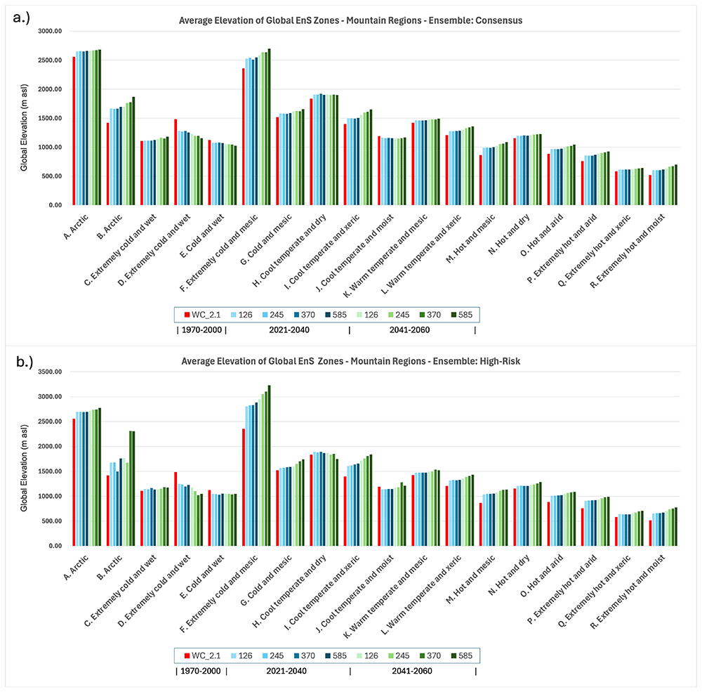
Figure 8. Global Average Elevation of Ens Bioclimatic Zones for One Historical and Two Future Time Periods.
Global average elevation of Ens bioclimatic zones for one historical (Baseline: WC_2.1: 1970–2000) and two future time periods (2021–2040; 2041–2060) showing results for two multi-model majority ensembles: a.) Consensus and b.) High-Risk. Only areas classified as a mountain region74 are included in this analysis.
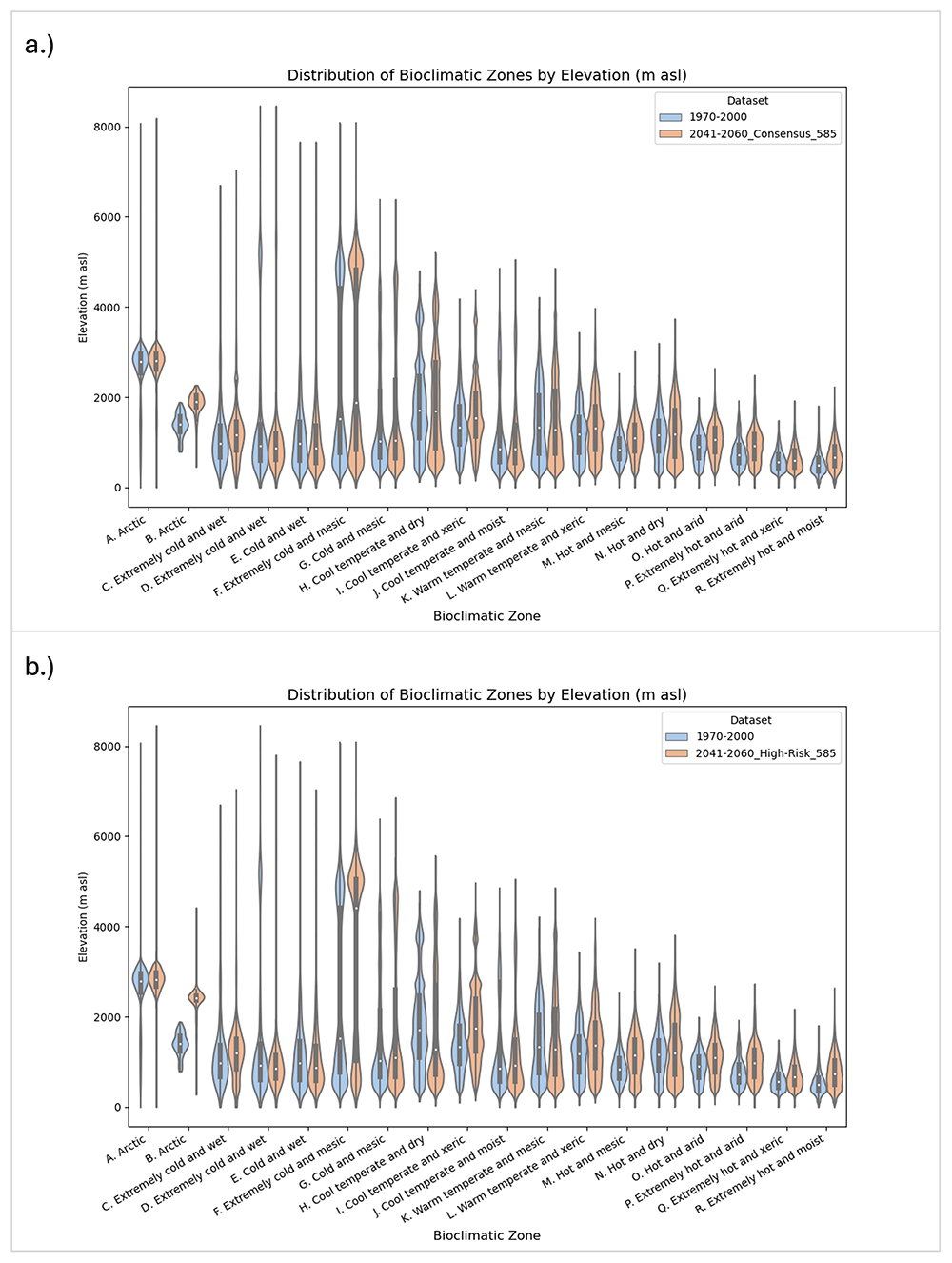
Figure 9. Global Distribution of EnS Bioclimatic Zones by Elevation for One Historical and One Future Time Period.
Global Distribution of Ens Zones Bioclimatic Zones by Elevation (m asl) for One Historical and One Future Time Period (2041–2060), showing results for two majority multimodel ensembles: a.) Consensus; and b.) High-Risk, evaluated for the SSP 5-8.5 scenario. Only areas classified as a mountain region74 are included in this analysis.
Elevational increases are even more pronounced in the High-Risk ensemble, where several zones exhibit vertical displacements exceeding 800 m by mid-century. Arctic Zone B increases to 2,307 m, an upslope migration of ~885 m, while the “Extremely Cold and Mesic” zone reaches over 3,228 m — an increase of ~871 m from its baseline. The “Cool Temperate and Xeric” Zone I, typically found in montane dry forests and steppe uplands, also shifts up by ~439 m. These values highlight the thermal sensitivity of montane ecosystems and point to a strong vertical restructuring of vegetation belts and ecological zones. Elevational shifts are among the most rapid and spatially compressed ecological responses to climate change86–88.
These projected large-scale upslope shifts of bioclimatic zone observed in this study are consistent with empirical studies and modelled projections in key mountainous biodiversity hotspots. For example:
• In the Tropical Andes, elevation gains exceeding 300 m imply substantial displacement of high-elevation endemics89, where many species are already restricted to narrow elevational bands.
• In the East African Highlands, shifts of 200–270 with steep terrain and limited elevation range exacerbate habitat compression risks90.
• The Hindu Kush–Himalayan region shows subalpine and alpine belt expansion by ~250 m, altering glacial hydrology, species distribution, and alpine plant communities91,92.
• The Western Ghats and Eastern Arc Mountains, showing rapid upslope shift (~180–220 m) with limited available elevational range, are globally significant biodiversity refugia with high endemism and are particularly vulnerable to vertical habitat loss90,93.
Consistent upslope highlight elevational compression, whereby land area diminishes rapidly with altitude, increasing competition for limited habitat and raising extinction risks for montane specialists81,82,86–88. In areas such as the Sierra Madre of Central America or Eastern Arc Mountains, the vertical narrowing of suitable climate space is expected to lead to range truncation and loss of high-elevation climate refugia80,94.
In thermal terms, the magnitude of vertical change observed across mountain regions — often equivalent to 3–5°C of warming — ranks among the most extreme global spatial (ecological) reorganizations, highlighting the vulnerability of mountain ecosystems to global climate change, and foretelling an extended period of biotic and ecosystem perturbation in mountainous regions with potential species decline and extinction81,82,87,88.
Compositional shifts in bioclimatic zones
Compositional stability refers to the proportion of a bioclimatic zone that retains its original classification over time; conversely, compositional turnover indicates the extent to which a zone’s baseline area transitions into other bioclimatic categories due to changing temperature and moisture regimes. Using the EnS WC 2.1 baseline (1970–2000) as the primary reference, comparison with the 2041–2060 projections under the high-emissions SSP5–8.5 scenario reveals distinct and systematic patterns of zonal reorganization (Table 8; Figure 10). Across both the Consensus and High-Risk ensembles, cooler and mesic zones exhibit high rates of internal turnover, while tropical and arid zones show comparatively higher, but still declining, stability (Figure 10).
Table 8. Compositional Stability of Historical EnS Bioclimatic Zones.
Compositional stability of historical EnS zones (Baseline WC_2.1; 1970-2000), expressed as percent of area (%) globally which shifts to a different EnS zone for two future projected time periods (2021-2040; 2041-2060), evaluated across the four Shared Socioeconomic Pathways (SSP 1-2.6; 2-4.5; 3-7.0; 5-8.5).
| Percent of EnS Zone Shifting to Different Zone (%) | 2021–2040 | 2041–2060 |
|---|
| Model | Baseline: WC_2.1. SSP: | 126 | 245 | 370 | 585 | 126 | 245 | 370 | 585 |
|---|
| Consensus | A. Arctic | 22 | 23 | 22 | 24 | 26 | 29 | 31 | 33 |
| B. Arctic | 80 | 70 | 76 | 83 | 90 | 93 | 89 | 94 |
| C. Extremely cold and wet | 27 | 27 | 26 | 28 | 30 | 32 | 33 | 37 |
| D. Extremely cold and wet | 38 | 38 | 35 | 39 | 44 | 48 | 50 | 54 |
| E. Cold and wet | 30 | 31 | 28 | 32 | 36 | 40 | 42 | 46 |
| F. Extremely cold and mesic | 53 | 53 | 49 | 56 | 65 | 72 | 74 | 82 |
| G. Cold and mesic | 66 | 67 | 62 | 70 | 79 | 84 | 85 | 90 |
| H. Cool temperate and dry | 78 | 78 | 75 | 81 | 89 | 93 | 93 | 96 |
| I. Cool temperate and xeric | 78 | 78 | 75 | 83 | 92 | 95 | 97 | 99 |
| J. Cool temperate and moist | 73 | 73 | 70 | 76 | 83 | 86 | 87 | 90 |
| K. Warm temperate and mesic | 79 | 79 | 76 | 82 | 90 | 93 | 94 | 96 |
| L. Warm temperate and xeric | 85 | 86 | 86 | 90 | 94 | 99 | 99 | 100 |
| M. Hot and mesic | 78 | 78 | 78 | 82 | 86 | 89 | 89 | 92 |
| N. Hot and dry | 82 | 82 | 81 | 85 | 91 | 94 | 95 | 98 |
| O. Hot and arid | 100 | 100 | 100 | 100 | 100 | 100 | 100 | 100 |
| P. Extremely hot and arid | 96 | 97 | 97 | 99 | 100 | 100 | 100 | 100 |
| Q. Extremely hot and xeric | 53 | 53 | 52 | 56 | 65 | 71 | 73 | 78 |
| R. Extremely hot and moist | 71 | 72 | 71 | 76 | 83 | 91 | 93 | 95 |
| High-Risk | A. Arctic | 26 | 25 | 28 | 27 | 31 | 35 | 46 | 42 |
| B. Arctic | 96 | 98 | 99 | 100 | 99 | 95 | 100 | 92 |
| C. Extremely cold and wet | 36 | 35 | 34 | 34 | 41 | 41 | 43 | 44 |
| D. Extremely cold and wet | 53 | 54 | 62 | 57 | 62 | 65 | 79 | 73 |
| E. Cold and wet | 49 | 50 | 50 | 53 | 59 | 64 | 69 | 73 |
| F. Extremely cold and mesic | 80 | 81 | 82 | 84 | 89 | 94 | 96 | 97 |
| G. Cold and mesic | 88 | 89 | 90 | 91 | 93 | 96 | 98 | 99 |
| H. Cool temperate and dry | 94 | 95 | 95 | 96 | 97 | 98 | 99 | 99 |
| I. Cool temperate and xeric | 97 | 98 | 98 | 99 | 100 | 100 | 100 | 100 |
| J. Cool temperate and moist | 88 | 89 | 90 | 91 | 93 | 95 | 96 | 97 |
| K. Warm temperate and mesic | 93 | 94 | 94 | 95 | 97 | 98 | 99 | 99 |
| L. Warm temperate and xeric | 97 | 98 | 97 | 99 | 99 | 100 | 100 | 100 |
| M. Hot and mesic | 89 | 90 | 90 | 91 | 94 | 95 | 96 | 97 |
| N. Hot and dry | 94 | 95 | 95 | 97 | 98 | 99 | 100 | 100 |
| O. Hot and arid | 100 | 100 | 100 | 100 | 100 | 100 | 100 | 100 |
| P. Extremely hot and arid | 100 | 100 | 100 | 100 | 100 | 100 | 100 | 100 |
| Q. Extremely hot and xeric | 71 | 72 | 70 | 73 | 80 | 85 | 89 | 92 |
| R. Extremely hot and moist | 91 | 93 | 93 | 94 | 96 | 96 | 96 | 96 |
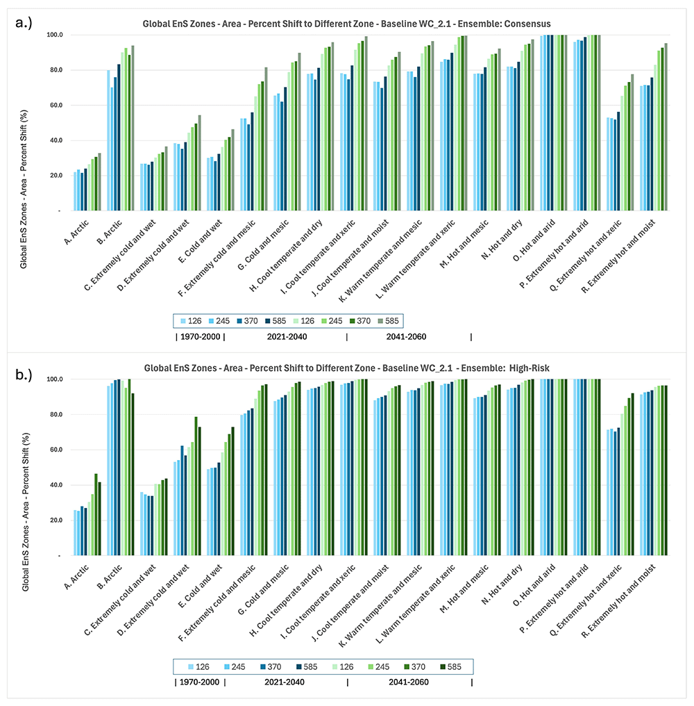
Figure 10. Compositional Shifts of Ens Bioclimatic Zones.
Compositional shifts of the EnS bioclimatic zones, globally, showing the area within an EnS zone that shifts to a different EnS zone (Area – Percent Shift (%)), in comparision with the 1970–2000 baseline (WC_2_1), for the Consensus and the High-Risk multi-model ensembles, across four Shared Socio-Economic Pathways (SSP: 1-2.6; 2-4.5; 3-7.0; 5-8.5).
Under both the Consensus and High-Risk ensembles, cold and montane bioclimatic zones exhibit significant vulnerability to compositional turnover by mid-century under SSP5–8.5 forcing (Figure 11). The Arctic (A) zone, encompassing high-latitude tundra and polar deserts across Siberia, Canada, and Greenland, retains 67% of its original bioclimatic classification under the Consensus model, but drops to 58% under the High-Risk. The Extremely Cold and Wet (C) zone, associated with glaciated coastal regions of Antarctica and alpine snowfields in the Rockies and Alps, retains more than 63% under Consensus and about 51% under High-Risk, indicating accelerated destabilization of snow-dominated landscapes. The Extremely Cold and Wet (D) zone, representative of permanent snow and glacial margins in high-elevation settings like the Andes and the Himalayas, retains just 45% under Consensus and about 36% under High-Risk projections. The Cold and Wet (E) zone, covering boreal forests and subarctic peatlands in Eurasia and North America, retains just over 50% compositional stability under Consensus, declining to 43% under High-Risk, reflecting the progressive transition of these cold-moist systems into warmer or drier classifications. The Extremely Cold and Mesic (F) zone, encompassing cold steppes and tundra margins, is highly unstable, retaining only 18% under Consensus and dropping further to nearly 12% under High-Risk scenarios. These patterns underscore the heightened sensitivity of cold, moisture-dependent systems to climate warming, and suggest that even relatively resilient polar and montane environments face increasing risks of fundamental ecological reorganization as global warming intensifies.
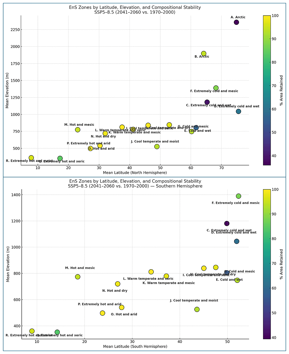
Figure 11. Distribution of EnS Bioclimatic Zones by Latitude, Elevation, and Compositional Stability.
Distribution of Ens bioclimatic zones by latitude, elevation, and compositional stability, showing the mean latitude and elevation of the 1970–2000 baseline time period (WC_2.1), and a comparision of the compositional stability (% Area Retained) with the Consensus Ensemble for the Shared Socio-Economic Pathway 8.5 (SSP: 5-8.5), for both the southern and northern hemispheres.
Mid-latitude bioclimatic zones exhibit exceptionally high compositional turnover by mid-century under SSP5–8.5 forcing. The Cool Temperate and Moist (J) zone—covering humid temperate forests in Europe, eastern Asia, and the Pacific Northwest—shows 90.4% turnover under the Consensus model and 96.6% under High-Risk projections. Similarly, the Warm Temperate and Mesic (K) zone, spanning Mediterranean-type ecosystems, moist subtropical highlands, and key agricultural regions such as southern Europe, southern China, and the southeastern United States, records 96.5% turnover under Consensus and 98.8% under High-Risk. These results indicate near-total bioclimatic shifting and turnover across mid-latitude humid zones, with implications for biodiversity, food security, and ecosystem stability82,95,96. The loss of climatic stability in these densely populated and highly productive zones poses escalating environmental and socio-economic challenges for global food security, regional sustainability and local livelihoods.
Tropical and arid bioclimatic zones exhibit exceptionally high zonal turnover, which may challenge previous assumptions of their relative resilience. The Extremely Hot and Moist (R) zone, characteristic of humid equatorial lowlands such as the Amazon Basin, Congo Basin, and equatorial Southeast Asia, retains less than 4.8% of its baseline extent under Consensus projections, dropping to just 1.0% under High-Risk scenarios. Similarly, the Hot and Dry (N) zones, encompassing semi-arid regions across southern Africa, interior Australia, and parts of the Indian subcontinent, retain only 2.5% of their baseline identity under Consensus and are nearly entirely reclassified under the High-Risk ensemble. The Hot and Arid (O) zones, which cover core desert systems such as the Sahara, Arabian Peninsula, and western Australia, experience virtually complete turnover under both model ensembles. These findings indicate that even tropical and subtropical zones, historically considered more compositionally stable due to their climatic extremity, are projected to undergo significant ecological transformation under continued high-emissions trajectories. The results suggest substantial bioclimatic and biotic perturbation of both hot humid, and arid systems globally, with implications for biodiversity persistence, carbon cycling, and regional climate feedbacks95,97,98.
Discussion
Overview of results
Through application of the EnS framework, this study has produced a high-resolution, globally consistent depiction of how bioclimatic envelopes are shifting across landscapes and across the globe. Our results show clear trends: contraction of cooler and mesic zones, poleward and upslope migration of many mid-latitude zones, and expansion of hotter and more arid conditions. Compositional analyses show relatively higher zonal stability in tropical and subtropical regions, but high vulnerability and turnover in temperate, montane, and high-latitude systems. The projected shifting of the bioclimatic envelopes and associated microclimatic and ecological niches, and in some cases stochastic non-contiguous movement of bioclimatic conditions across landscapes, continents, and the globe, will have, and is having, profound ecological and socioeconomic implications. The compositional and elevational shifts, and the more general poleward migration of bioclimatic zones evident from the analysis suggest an extended period of bioclimatic, ecological and biotic perturbation80, with widespread impacts for ecosystem functioning and on the provision of ecosystem services across all continents and biomes. These projected rapid transitions to locally novel bioclimatic conditions will impact not only on natural ecosystems, wildlife and wildlife habitat, plant communities, species distributions, and pollinator synchronization, but also, notably, cause the displacement or suitability of current agriculturally suitable zones, particularly in temperate regions, as well as areas suitable for human habitation. Tropical regions may become increasingly difficult for human activities, especially for those working outside99 or other vulnerable populations, with implications for economic productivity. Taken together, the results of the global analysis and the projected trends and observed patterns confirm we are currently in a profound period of ecological perturbance and fundamental reorganization of the Earth’s bioclimatic zones in response to global climate forcing. The ensemble results highlight both the magnitude of expected changes and the variability across space and models—critical information for forecasting ecosystem transitions and delineating future potential risk space, guiding conservation priorities, and developing regional sustainable development and climate adaptation strategies.
This study presents global results (at the EnS “zone” level) to illustrate the general geographical applicability and the “big picture” insight that can be had at the global scale with the EnS methodology, as well as demonstrating the general utility of the resultant EnS database of CMIP6 future projections. However, the relatively high spatial resolution of this dataset, applied at the finer scales of the “EnS “strata” (as opposed to zonal) level, allows (with some care given for increased local uncertainly) the application of this methodology to more defined, specific regional and local geographical contexts, and/or focused on specific thematic areas of interest. While the global analysis illustrates the power of the EnS methodology to integrate and interpret climate projections, in this case the CMIP6 ESM, in more ecologically and easily interpretable terms, this capacity for interpretive insight is specifically more evident at the regional to local levels, where bioclimatic homologues may be easily recognized and intuitively understood by stakeholders, policymakers, and the public.
The regional variability and local nature of bioclimatic strata and their associated biotically relevant trends underscore the need for regional, local, and adaptive land management strategies (and communication) to mitigate the impacts of rapidly shifting bioclimatic envelopes and environmental regimes. The spatially explicit results produced by this framework (at 30 arc seconds resolution) are well suited for national and sub-national adaptation planning, conservation prioritization, and climate-smart agriculture applications. While the variability between climate models and scenarios further emphasizes the spatial and temporal heterogeneity and uncertainty of modeled and projected change, much of the results reported in this study align with documented trends from empirical sources suggesting the EnS projections as ecologically realistic and empirically corroborated, at least in terms of trends, if not magnitude.
Correspondence with observed trends and empirical change
The spatial and compositional transitions identified through the EnS framework correspond strongly with empirical observations of climate-driven ecological change, offering support for the framework’s predictive and diagnostic robustness. Multiple independent datasets and monitoring networks have documented latitudinal and elevational shifts in species distributions, ecosystem boundaries, and vegetation dynamics that mirror the projected shifting and reorganization of EnS zones. Upslope migration of alpine plant communities in the European Alps, Tropical Andes, and Himalayas have been documented with observed mean elevational shifts of ~0.3–0.5 m/year75,88,100,101. While these rates are notably lower than the ~2.0–5.8 m/year upslope averaged velocity projected for mountain EnS zones (200–300 meters by mid-century), the directional alignment supports the idea that high-elevation ecosystems are already undergoing climate-driven reorganization and responding to shifting bioclimatic conditions, and the potential lag with species’ ability to move and adapt. MODIS-based vegetation productivity indices show greening trends in high-latitude ecosystems (e.g., tundra and boreal forest transition zones) indicative of warming-induced northward expansion75, while thermal degradation of permafrost and drying of peatlands are consistent with compositional shifts in the “Cold and Mesic” and “Cold and Wet” EnS zones. The high spatial resolution of the EnS CMIP6 ensembles (and the datasets in the Future_Global_Ens Database) reveal fine-scale variation that aligns with observed sub-regional trends, for example, the compression of upper-montane habitats and expansion of subtropical drylands in East Africa and South Asia.
In contrast to the extensive compositional turnover projected for temperate and cold bioclimatic zones, tropical and arid systems exhibit somewhat greater internal inertia under future climate scenarios. Nevertheless, substantial internal reorganization and zonal shifting is projected across tropical forests biomes, semi-arid regions, and desert systems, suggesting that these ecosystems, long considered climatically more resilient, are increasingly vulnerable to intensified warming and hydrological stress. These findings align with the traditional perception of tropical and arid zones as ecologically stable under climate change, up to a point, highlighting that even regions already characterized by thermal or moisture extremes are susceptible to significant internal transformation13,30. Observed patterns of forest degradation, desert expansion, and altered precipitation regimes in tropical and subtropical regions further reinforce the likelihood of profound future shifts98. The emerging evidence suggests that while tropical and arid systems may resist complete zonal reclassification longer than temperate and montane ecosystems, they are nevertheless highly vulnerable to the destabilizing effects of continued global warming5,13,30.
The EnS methodology has demonstrated high internal accuracy when reconstructed from climate inputs, with kappa statistics exceeding 0.916 and user accuracy above 91% in comparison with the original GEnS dataset10,102. Comparative studies using alternative classification methods—such as Random Forests or neural networks—have shown similar spatial patterns but lower overall agreement with established bioclimatic boundaries11. EnS also shows strong structural concordance with other ecological zonation frameworks, including Köppen-Geiger classifications and WWF terrestrial ecoregions12,103, while offering the advantage of being statistically derived and ecologically interpretable8. The availability of two historical time periods offers a opportunity to “ground truth” observed climate change over a recent decade: zones known to be experiencing ecological transitions (e.g., the Tibetan Plateau, the Canadian boreal belt, and the Eastern Himalayas) exhibit high compositional turnover, showing the EnS abilituy to monitor real-world change.
Elevational displacement: observed trends and modeled velocity
The EnS ensemble analysis projects significant upslope displacement of mountain bioclimatic zones under future climate scenarios, with modeled elevation gains of 110–180 meters under the majority ensemble and 250–320 meters under the high-risk ensemble by mid-century (2041–2060). These values correspond to an annual elevational velocity of ~2.0–3.3 m/year (Consensus) and 4.5–5.8 m/year (High-Risk). These rates substantially exceed observed biological responses, such as those documented by the GLORIA network, which has tracked alpine plant communities shifting ~2–5 meters per decade (~0.3–0.5 m/year) across mountain systems including the European Alps, Tropical Andes, and Himalayas88,100. Similar lags have been reported in avian and insect communities in the East African Highlands, where species richness and composition are changing more slowly than underlying climate envelopes, and in the Hindu Kush-Himalaya, where upslope tree line movement averages less than 2.6 meters per year104 over recent decades.
This discrepancy highlights the difference between the rapid movement of bioclimatic conditions and the lagged response of ecological communities due to dispersal limitations, geo-ecolgoical constraints, and biotic interactions80,83,88,94,105,106. EnS zone shifts reflect changes in climate suitability, providing an early-warning signal of where ecosystems may undergo future restructuring, even if biotic responses are not yet evident. The projected rapid upslope velocity of EnS elevation change underscores the vulnerability of topographically constrained systems94, especially in regions with steep gradients and limited habitat availability at higher elevations, such as the Eastern Arc Mountains, Central American Highlands, and many other mountain regions. In these cases, upward compression of EnS zones exacerbates risks of habitat loss and extinction107, particularly for endemic and range-restricted species80,94.
Both observed and projected results point to increased ecological risk with delayed mitigation and underscore the urgent need for climate- and elevation-informed conservation strategies, notably:
• Preservation of altitudinal corridors to facilitate species movement along elevation gradients,
• Protection of upper slope refugia and montane transition zones, which act as critical buffers for biodiversity under warming scenarios,
• Climate-aware restoration planning for degraded mountain systems, prioritizing future climate suitability and connectivity,
• Monitoring and early-warning systems to track shifts in vegetation zones and species range margins in real-time,
• Incorporation of elevational dynamics into protected area design, ensuring that conservation boundaries accommodate future upslope movement,
• Community-based adaptation strategies in montane landscapes, recognizing the dependency of upland communities on climate-sensitive ecosystems such as cloud forests and montane grasslands.
Utility of environmental stratification for climate-resilient planning
The results presented here illustrate the power of environmental stratification to convert climate model outputs into actionable ecological insights. By combining high spatial resolution with interpretable and ecologically meaningful bioclimatic strata (and the GEnS taxonomy), EnS enables detailed analysis of bioclimatic change at scales relevant to decision-making, allowing for both global assessments and regional to locally specific applications. For instance, the identification of high-risk zones with low compositional stability or high spatial turnover provides direct inputs for prioritizing conservation efforts, land-use planning, and food security. Zones such as “Cold and Wet” and “Cool Temperate and Moist,” which show >50% transition rates in some regions, could serve as focal areas for various forms of resilience-building, habitat restoration, or assisted migration strategies. Essentially, all of the EnS bioclimatic strata (n=125) and all regions of the globe are undergoing rapid change, at various rates, and can benefit from an improved understanding of the direction and magnitude of that change. By focusing on statistically and bioclimatically coherent spatial units, EnS avoids many of the limitations associated with raw climate variables or broad biome models, offering enhanced interpretability for policy and practice. By providing baselines and quantifying the spatial rate at which ecologically relevant bioclimatic conditions are shifting, EnS provides a metric with utility for environmental and biodiversity conservation, informing the design of biodiversity corridors, climate refugia, assisted migration strategies in mountain regions where climate tracking failure is likely80,83,108, as well as local adaptation, rural landuse, and urban planning. Importantly, in terms of food security, the type of results provided by this analysis are of great utility for developing agricultural sustainability and resilience, plant breeding for future conditions, habitat restoration, and species selection for agroforestry47,109 or other long-rotation tree or forestry plantations.
Applications across sectors: conservation, agriculture, and sustainable development
The implications of shifting EnS zones, although not specifically analyzed or articulated in this global study, span multiple sectors critical to sustainability. In conservation, for example, environmental stratification can identify regions of high vulnerability, ecological novelty, or future refugia, guiding the design of effective protected area networks and prioritizing areas for habitat connectivity and species migration corridors18,20. Likewise, for the agricultural sector, understanding future bioclimatic conditions will be essential to inform plant breeding, climate-smart farming systems, crop suitability assessments, and ensure food security as landscape change accelerates22,110,111. As an example, results highlight particularly rapid zonal transitions in montane East Africa and the Himalayan foothills, regions where smallholder systems are highly sensitive to climate variability and food security is already an issue. For supporting sustainable development, adaptation and strategic planning, the EnS methodology enables the delineation of both future climate and “climate risk spaces” that delineate ecological vulnerabilities, helping target adaptation efforts, and identify regions where transformative adaptation will be required28. An interpretable understanding of shifting bioclimatic conditions is required to inform effective Nature-based Solutions (NbS) and ecosystem-based adaptation (EbA) strategies, providing spatially explicit baselines for monitoring how changing conditions might impact the provisioning of ecosystem services that underpin resilience in both human and natural systems25,26.
From global to local: a framework for regionalization
While this study provides a global overview, the greatest utility of the EnS methodology lies in its regional and local application. Because the EnS framework is scale independent, it can be applied to any climate dataset or spatial extent, including at national and subnational scales, enabling local decision-makers to assess climate risks and opportunities with spatial specificity. Downscaling and customizing the methodology to local environmental gradients and policy contexts enhances relevance for regional land-use planning, adaptation financing, agricultural zoning, and biodiversity offsets. High-resolution regional EnS analyses have already demonstrated utility in areas such as Southeast Asia12,17,20,47, the Hindu-Kush Himalayas17,47,103,109,112, and Central Asia113,114, but more widespread adoption would improve integration of current and future rapidly changing bioclimatic conditions across global frameworks, e.g., the SDGs, UNFCCC National Adaptation Plans (NAPs), and the Post-2020 Global Biodiversity Framework115.
Future directions and integration with emerging technologies
Advances in earth observation and remote sensing technologies, AI-driven ecological modeling, and big data analytics offer opportunities for enhancing and applying the EnS framework. Coupling environmental stratification with predictive modeling and monitoring of ecosystem responses (e.g., vegetation phenology, land degradation, species shifts) can provide or improve early warning systems. Integration with socio-economic datasets also enables deeper analysis of coupled social-ecological systems under climate stress18. The EnS framework is well-positioned to serve as a bridge between climate science and decision-making, especially when combined with participatory and interdisciplinary approaches to adaptation planning. As the availability and quality of high-resolution geospatial earth observation, climate and other datasets advance and become more generally accessible, the opportunity to combine this methodology using a set of improved data inputs with advanced geospatial analysis (e.g. artificial intelligence classification methods incorporating a greater range of inputs) will allow for more topically relevant questions and more targeted results in the future.
Conclusion
The Environmental Stratification (EnS) methodology offers a powerful, scalable, and ecologically realistic framework for interpreting the complex spatial patterns of climate change. By integrating key climatic variables into discrete, interpretable bioclimatic zones, EnS transforms raw model outputs into ecologically meaningful insights that are accessible to researchers, practitioners, policymakers, and the general public. This study demonstrates that EnS methodology is capable of revealing both broad-scale global patterns, such as the poleward and upslope migration of climate zones, and fine-grained regional changes that are directly relevant to local adaptation planning. The framework not only reveals the magnitude and direction of projected shifts but also identifies zones of high turnover and relative stability, offering critical guidance for prioritizing conservation and land management efforts.
What distinguishes EnS from other climate classification approaches is its flexibility and interpretability. It functions effectively across spatial scales and climate model ensembles, making it well-suited for scenario-based planning. Its outputs can be used to assess climate risk exposure, ecological vulnerability, and land-use suitability under current and future conditions. The compositional and spatial analyses enabled by EnS have particular utility for climate-sensitive sectors such as agriculture, forestry, biodiversity conservation, and sustainable development. Because it integrates ecological processes and environmental gradients intuitively, EnS facilitates communication with local stakeholders and decision-makers, bridging the often-wide gap between complex climate data and actionable planning tools.
The utility of environmental stratification methodologies, and the EnS framework in particular, will increase with the increased availability of higher resolution spatial and temporal data, and as climate adaptation and mitigation become more urgent and more spatially targeted. The purely statistically based approach of the EnS methodology allows integration of new earth observation and remote sensing data products, real-time monitoring systems, and socio-economic datasets, enabling deeper insight into coupled human-natural systems. By providing a common ecological language across scales—from global assessments to community-level planning—EnS can serve as a foundational tool for anticipating ecological transitions, identifying opportunity spaces for adaptation, and supporting transformative resilience strategies in the face of rapid climate change.








