Topology-based analysis and optimization for agent fleet behavior

Javier Perera-Lago; Victor Toscano-Duran; Alvaro Torras-Casas; Rocio Gonzalez-Diaz

doi:10.12688/openreseurope.20760.1

Topology-based analysis and optimization for agent fleet behavior

Article

Authors & roles Authors

Peer review record Peer review

Metrics

Cite

Section

Method Article

Published

July 29, 2025

DOI

https://doi.org/10.12688/openreseurope.20760.1

Versions

July 29, 2025 (Version of Record 1.0)

French Agence Nationale de la Recherche

Grant ID(s): ANR-22-CPJ1-0047-01
European Commission

Grant ID(s): 101070028

Views

Downloads

Citations

See full metrics

Computational topology, topological data analysis, persistent entropy, persistent divergence, partial matchings, reliability, explainability, agent fleet behavior.

Abstract

We introduce novel topological methods for analyzing the behaviors and navigation of an agent fleet. Our goal is to understand and enhance the evolution of agent fleet behaviors to minimize unintended behaviors, such as collisions and deadlocks. Understanding the dynamics of the agent fleet enables us to predict safer and more efficient routes for their deployment. To achieve this, we propose employing geometric-topological approaches such as graph-based techniques, Vietoris-Rips filtrations, persistent homology, matching diagrams, and persistent entropy. These methods leverage the geometric and topological structure of the data, allowing us to capture spatial and relational patterns in agent fleet behaviors and configurations. Unlike classical approaches, which often rely on predefined features or statistical assumptions, geometric-topological-based techniques offer an interpretable framework that highlights qualitative differences in the dynamics of the agent fleet. The added interpretability and the ability to capture intrinsic spatial structures make these techniques particularly suitable for characterizing different agent fleet behaviors and ensuring safe and efficient simulation runs. This work is part of the European Project “REliable & eXplainable Swarm Intelligence for People with Reduced mObility - REXASIPRO”.

Corresponding author

Javier Perera-Lago

0009-0009-4536-4020

jperera@us.es

Grant information

This project was supported in part by the European Union HORIZON-CL4-2021-HUMAN-01-01 under grant agreement 101070028 (REXASI-PRO) and the French Agence Nationale de la Recherche through the project reference ANR-22-CPJ1-0047-01.

This work is licensed under a Creative Commons Attribution 4.0 International License.

First version published

July 29, 2025 (https://doi.org/10.12688/openreseurope.20760.1)

Latest version published

July 29, 2025 (https://doi.org/10.12688/openreseurope.20760.1)

1 Overview

We develop novel topological methods for the analysis of discrete models of fleet behavior. Our aim is the improvement of such models via topological signatures to make them more reliable, avoiding unintended behaviors. Understanding the model’s dynamics allows us to predict safer (i.e., with fewer agent collisions) and more efficient (i.e., with fewer agent deadlocks) navigation behaviors. To achieve this,we propose employing geometric-topological approaches such as graph-based techniques, Vietoris–Rips filtrations, persistent homology, matching diagrams, and persistent entropy. We have implemented and tested our methods under the Navground navigation simulator¹, which is a library of 2-dimensional navigation algorithms that provide a common API to interact with dynamic obstacle avoidance behaviors for multi-agent systems. All examples included in this paper are based on simulation runs of ground robot fleets, such as smart wheelchairs. This work is part of the European Project REXASIPRO^2,3.

The work has been divided into three main research lines, based on the goal we plan to solve.

1. Navigation improvement through graph-based behavior modulation. The objective here is to enhance the safety and efficiency of the social navigation algorithms available in the Navground navigation simulator by employing a behavior modulation approach that utilizes graph theory to model the environment, enabling the detection and avoidance of negative events, such as collisions and deadlocks.
2. Capturing stable topological characteristics of the agent fleet. The main objective here is to quantify the diversity and spatial distribution of the agent movement patterns. For this purpose, we capture robust topological features of the agent fleet using persistent entropy. This is particularly useful for identifying complex behaviors and configurations (such as clustering and movement patterns) that emerge within the system. Additionally, we propose a machine learning-based approach to distinguish between safe and unsafe simulations, i.e., those with and without collisions between agents. We extend this approach to identify efficient simulations, i.e., those with and without deadlock situations, as well as compliant simulations, to ensure both safety and efficiency. Finally,we analyze the relationship between the rules derived by these machine learning models and the internal simulation parameters to configure safe and efficient navigation scenarios. This approach contributes to improving the reliability of artificial intelligence (AI) systems by incorporating explainable AI techniques. In particular, we combine machine learning methods with probabilistic models and the generation of conformal safety regions. These tools quantify uncertainty and offer interpretable guarantees about model behavior, key aspects for building trustworthy and transparent systems.
3. Navigation behavior characterization with partial matchings. We introduce partial matchings among time-varying simplicial complexes and study the concept of persistent divergence, which quantifies how surprising the new barcode is compared to the previous one. In other words, the aim is to detect and measure significant differences between such time-varying simplicial complexes. Firstly, given that each time step represents the spatial configuration of agents in the environment, this technique allows us to capture meaningful changes in their spatial relationships throughout the simulation. By applying partial matching in this realistic use-case scenario, we characterize different agent fleet behaviors and configurations, reinforcing the practical value of our foundational approach in challenging settings. Secondly, we focus on studying the topological characteristics of complete simulation runs. To do so, we generate several different types of time series that analyze the similarities between the positions and trajectories of the agents and give us an idea of the degree of order or chaos within the navigation behavior. Moreover, we compare the generated time series to check which navigation behaviors best order the agents. In addition, we perform a quantitative analysis using clustering techniques to determine whether it is possible to distinguish different behaviors based on these time series. This approach helps detect changes in agent fleet behaviors based on similar movement patterns, providing deeper insights into the dynamics of the system.

The paper is organized as follows: Section 2 introduces the concepts necessary to understand the methodology and experiment parts, including key concepts about graph theory, simplicial complexes, persistent homology, matching diagrams, and time series. Section 3 provides an overview of the Navground navigation simulator, describing some of the different scenarios and behaviors it supports and which we use in our experiments, while performing an initial statistical analysis to distinguish behaviors and relate them to events such as collisions or deadlocks. Section 4, Section 5, and Section 6 explain the methodology followed and the experiments performed for each of the research lines mentioned above, respectively, and present in detail the results obtained in each case. Section 7 summarizes the main conclusions drawn from the research done. Finally, in Section 7, we provide links to all the code developed for the experiments presented in this paper. Table 1 contains a list of acronyms that will be used throughout the paper.

Table 1. Acronyms.

Acronym	Expanded form
ACC	Accuracy
AI	Artificial intelligence
CP	Conformal prediction
DL	Deep learning
DTW	Dynamic time warping
F1	F1-score
FNR	False negative rate
FPR	False positive rate
HL	Human like
HRVO	Hybrid reciprocal velocity obstacle
KDE	Kernel density estimation
MEB	Minimum enclosing ball
ML	Machine learning
ORCA	Optimal reciprocal collision avoidance
PCA	Principal component analysis
PE	Persistent entropy
PS	Probabilistic scaling
REXASI-PRO	Reliable & explainable swarm intelligence for people with reduced mobility
SFM	Social force model
SVM	Support vector machine
TDA	Topological data analysis
TNR	True negative rate
TPR	True positive rate
UMAP	Uniform manifold approximation and projection
VR	Vietoris-Rips
XAI	Explainable artificial intelligence

2 Background

In recent years, there has been significant interest in applying Topological data analysis (TDA) tools to various domains, including the analysis of dynamic systems and behaviors, since TDA provides powerful tools for understanding complex structures and patterns in data that traditional methods often struggle to capture effectively^1,2. Topological data analysis, particularly persistent homology, has emerged as a valuable approach for studying the geometry and connectivity of datasets that evolve over time or space³. Persistent homology enables the identification of robust topological features that persist across different scales, offering insights into the underlying structure of complex systems⁴. The primary objective of using TDA tools like persistent homology and persistent entropy in the context of fleet behavior modeling is to achieve a more nuanced understanding of system dynamics. These tools enable the characterization of distinct patterns and structures in the movement behaviors of different agents (e.g., pedestrians, wheelchairs) within the environment. By identifying and quantifying these patterns, researchers can predict potential conflicts, optimize routes for agent displacement, and ultimately improve the safety and efficiency of navigation strategies.

In this section, we recall the mathematical background needed for understanding the methodology used in the following sections. We provide key concepts about graphs (Subsection 2.1), time series analysis (Subsection 2.2), simplicial complexes (Subsection 2.3), persistent homology (Subsection 2.4), triplet merge trees (Subsection 2.5), matching diagrams (Subsection 2.6), and topological descriptors (Subsection 2.7).

2.1 Graphs, paths and connectedness

Below, we explain some basic concepts from graph theory useful to understand the methodology and experiments done in Section 4. These concepts are covered in any basic graph theory book, for example 5.

A graph is an ordered pair G = (V, E) where V = {v₁, v₂, . . . , v_n} is a finite non-empty set of elements called vertices and E ⊆ {{u, v} | u, v ∈ V and u ≠ v} is a set of unordered pairs of distinct vertices, called edges. When there is an edge {u, v} ∈ E, we say that the vertices u and v are adjacent.

Graphs model real-world problems effectively by abstracting details and emphasizing relationships. Moreover, their definition is simple and allows for a very clear visualization by drawing the vertices of V as points on a plane and the edges of E as curves between them, as the graphs in Figure 1.

Figure 1. Left: Visual representation of a graph G = (V, E) with V = {a, b, c, d} and E = {{a, b}, {a, c}, {b, c}}.

Right: subgraph G_C of the graph G generated by C = {a, b, d}.

Graph theory is very rich and extensive, but we only need to use a few basic concepts, such as paths, connectedness, and subgraphs. Let G = (V, E) be a graph. A path in G is a sequence of distinct vertices (p₀, p₁, . . . , p_k) such that p_i ∈ V for all i = 0, 1, . . . , k and {p_i−1, p_i} ∈ E for all i = 1, 2, . . . , k. In the graph G from Figure 1, (b, a, c) is a path but (a, d) is not because there is no edge {a, d} in E.

Two vertices u, v ∈ V are said to be path-connected if there is a path (p₀, p₁, . . . , p_k) in G such that u = p₀ and v = p_k (in this case we say that the path connects u and v). In the graph G from Figure 1, vertices b and c are path-connected because (b, a, c) is a path in G, while d is not path-connected to any vertex but itself (each vertex in v ∈ V is path-connected to itself considering the trivial path (v)).

A path-connected component of G is a maximal subset of vertices C ⊆ V such that for any pair of vertices u, v ∈ C, there exists a path in G connecting u and v. In otherwords, a path-connected component is a maximal set of mutually path-connected vertices. If G only has one path-connected component, it is said to be a path-connected graph. The graph G from Figure 1 is not path-connected because it has two separate path-connected components, which are C₁ = {a, b, c} and C₂ = {d}.

Given a subset of vertices C ⊂ V, we define the subgraph of G generated by C as the graph G_C = (C, E_C), where E_C = {{u, v} ∈ E | u, v ∈ C}. In Figure 1, we can see an example of a subgraph G_C generated by the subset of vertices C. A subgraph of G is a clique if every pair of its vertices is connected by an edge—in other words, it is a fully connected subgraph.

2.2 Time series analysis

Next, we provide some basic definitions related to time series, useful to understand the methodology and experiments given in Subsection 6.2.

Let T ⊂ ℝ be a set that we call the parametric set. A time series parameterized by T is a map X : T → V where V is some value set. Depending on the type of the parametric set, some time series have specific names and are studied differently. For example, when the parametric set T is an interval I ⊂ ℝ or when T = ℝ, the parameter and the time series are called continuous. On the other hand, if T = ℕ or T is a finite set, the parameter and the time series are called discrete. There may also exist time series with mixed-type parameters that do not fit into these two categories, but for our study, we do not need to consider them. Time series can also be distinguished by the value set V. If V = ℝ, the time series is called univariate, whereas if V = ℝ^d with d ≥ 2, the series is called multivariate.

Given a parameter t ∈ T, the term X(t) ∈ V is often denoted as x_t. Therefore, when the parameter is a finite set T = {1, 2, . . . , n}, the time series X is defined not as a function but as an ordered sequence of values X = {x₁, x₂, . . . , x_n}.

Similarity measures for time series. To find differences between the navigation behaviors using time series in Subsection 6.2, we first need to decide how we measure their similarity. We assume that the time series to be compared take values in the same set V and that we have an appropriate distance function d_V : V × V → ℝ⁺.

Now, suppose we have two time series X : T_X → V, Y : T_Y → V with parameter sets that are not necessarily equal. Therefore, to compare two time series, we cannot use the term-by-term difference between them. For this reason, we apply dynamic time warping (DTW)⁶. DTW is an algorithm that calculates the similarity between X and Y by searching for an optimal alignment between T_X and T_Y. Thanks to DTW, similarities can be found between time series even if they are delayed, have different lengths, or speeds.

Specifically, suppose T_X = {1, 2, . . . , N} and T_Y = {1, 2, . . . , M}. An alignment between T_X and T_Y is an ordered sequence of pairs p = ((a₁, b₁), (a₂, b₂), . . . , (a_ℓ, b_ℓ)), where:

(a_i, b_i) ∈ T_X × T_Y ∀i = 1, 2, . . . , ℓ;
(a₁, b₁) = (1, 1) and (a_ℓ, b_ℓ) = (N, M);
0 ≤ a_i+1 − a_i ≤ 1 and 0 ≤ b_i+1 − b_i ≤ 1, ∀i = 1, 2, . . . , ℓ − 1.

Let A(T_X, T_Y) be the set of all possible alignments between T_X and T_Y. The DTW distance between X and Y is:

d_{D T W} (X, Y) = \min_{p \in A (T_{X}, T_{Y})} \sum_{(a, b) \in p} d_{V} (x_{a}, y_{b}) .

Although the function d_DTW is positive, symmetric, and satisfies that d_DTW(X, Y) = 0 if and only if X = Y, it is not a true distance because it does not, in general, satisfy the triangle inequality.

Clustering evaluation for time series datasets. In Subsection 6.2, we group time series based on their similarities. To quantitatively assess the quality of this clustering, we use a well-established evaluation method: the silhouette score⁷.

Suppose that we have a time series dataset 𝔛 = {(X¹, y¹), . . . , (X^N, y^N)}, where Xⁱ is the i-th time series and yⁱ ∈ {1, . . . , m} is a label assigned to Xⁱ. We divide 𝔛 into m clusters where the n-th cluster is 𝔛_n = {(Xⁱ, yⁱ) | yⁱ = n} for n = 1, . . . , m. The silhouette indicates whether this division of 𝔛 into clusters is meaningful, that is, each time series is similar to the time series in its cluster but different from the time series in other clusters.

Specifically, given a time series Xⁱ ∈ 𝔛_n, we define:

a (X^{i}) = \frac{1}{| X_{n} | - 1} \sum_{X^{j} \in X_{n}, X^{i} \neq X^{j}} d_{D T W} (X^{i}, X^{j}), b (X^{i}) = \min_{n^{'} \neq n} \frac{1}{| X_{n^{'}} |} \sum_{X^{j} \in X_{n^{'}}} d_{D T W} (X^{i}, X^{j}) .

That is, a(Xⁱ) is the average of the distances between the time series Xⁱ and all those in its cluster 𝔛_n, while b(Xⁱ) is the average of the distances between Xⁱ and all the time series in the other clusters 𝔛_n′ with n′ ≠ n. Knowing a(Xⁱ) and b(Xⁱ) the silhouette value of Xⁱ is defined as:

s (X^{i}) = \frac{b (X^{i}) - a (X^{i})}{\max {a (X^{i}), b (X^{i})}} .

From this definition, it follows that −1 ≤ s(Xⁱ) ≤ 1. When a time series closely resembles those in its cluster, a(Xⁱ) is low and b(Xⁱ) is high, so s(Xⁱ) is close to 1. Conversely, if s(Xⁱ) is negative, this indicates that its similarity to elements from another cluster is greater than to those in its group, suggesting that the clustering is not well-formed. To assess whether the signals we have generated effectively separate the clusters 𝔛₁, . . . , 𝔛_m, we calculate the silhouette value for each time series and use the following summary metrics:

Silhouette score: the average of all silhouette values in the dataset.
$σ (X) = \frac{1}{| X |} \sum_{i} s (X^{i}) .$
Fraction of positive silhouettes: the fraction of elements in the dataset with a positive silhouette value.
$π (X) = \frac{| {(X^{i}, y^{i}) | s (X^{i}) > 0} |}{| X |} .$

2.3 Simplicial complexes

A topological space is a powerful mathematical concept for describing the connectivity of a space. Informally, a topological space is a set of points, each of them equipped with the notion of neighborhood. One way to represent a topological space is by decomposing it into simple pieces such that their common intersections are lower-dimensional pieces of the same kind. We use simplicial complexes as the data structure to represent topological spaces. See 2 for an introduction to these concepts.

An abstract simplicial complex 𝒦 can be seen as a generalization of the concept of graphs. It can be obtained by a nested family of simplices: a 0-simplex can be thought of as a point, a 1-simplex as an edge, a 2-simplex as a triangle, and a 3-simplex as a tetrahedron, and so on. Formally, 𝒦 is given by:

A set V of 0-simplices (also called vertices);
For each k ≥ 1, a set of k-simplices σ = {v₀, v₁, . . . , v_k}, where v_i ∈ V;
Each k-simplex has k + 1 faces obtained by removing one of the vertices;
If σ belongs to 𝒦, then all the faces of σ belong to 𝒦.

A simplicial complex K is a geometric realization of an abstract simplicial complex 𝒦. In this paper, both the abstract simplicial complex and its geometric representation are called a simplicial complex and denoted by K, to simplify the exposition.

Next, we introduce the Vietoris-Rips complex, a well-known construction of simplicial complexes in computational topology that is used to study the topological structure of a set of points in space. It is defined based on the pairwise distances between points, allowing us to capture the connectivity and shape of the set through simplices. The simplicity of its construction and the ability to control its dimension make this complex one of the most used, especially for high-dimensional datasets.

Precisely, let 𝒫 = {p₁, p₂, . . . , p_n} be a set of points in a metric space ℝ^d and r a positive radius. The Vietoris-Rips complex VR_r(𝒫) is defined as:

V R_{r} (P) = {σ \subseteq P | ‖ p_{i} - p_{j} ‖ \leq r for all p_{i}, p_{j} \in σ}

where ∥p_i − p_j∥ denotes the distance between points p_i and p_j. In other words, a simplex σ belongs to the Vietoris-Rips complex VR_r (𝒫) if the pairwise distance between every pair of points p_i, p_j ∈ σ is less than or equal to r. Specifically,

A 0-simplex of VR_r(𝒫) is a vertex p_i of 𝒫.
A 1-simplex (edge) between p_i and p_j exists in VR_r(𝒫) if ∥p_i − p_j∥ ≤ r.
A 2-simplex (triangle) among p_i, p_j, p_k exists in VR_r(𝒫) if ∥p_i − p_j∥ ≤ r, ∥p_j − p_k∥ ≤ r, and ∥p_k − p_i∥ ≤ r.
In general, a k-simplex exists in VR_r(𝒫) if the distance between every pair of points in the simplex is less than or equal to r.

Figure 2 shows an example of the Vietoris-Rips complex VR_r(𝒫) for a set 𝒫 in ℝ².

Figure 2. Vietoris-Rips complex example.

The black dots represent 0-simplices, while the yellow circles indicate the coverage regions of the ball centered at each point with radius r = 0.2. Blue lines depict edges connecting points whose coverage regions overlap, forming a 1-simplex. The light blue triangular region highlights a 2-simplex, where three points’ coverage regions intersect.

2.4 Persistent homology

Homology groups are algebraic structures that describe features of a topological space 𝒯. The k-th Betti number represents the rank of the k-dimensional homology group. Informally, for a fixed k, the k-th Betti number β_k counts the number of k-dimensional holes characterizing 𝒯: β₀ is the number of connected components, β₁ counts the number of holes in ℝ² or tunnels in ℝ³, β₂ can be thought of as the number of voids in geometric solids. In this work, we compute homology groups of simplicial complexes.

The generators of homology groups may arise from sampling artifacts (noise). To address this, we instead consider persistent homology. In this section, we briefly explain how this method works. For more information, we refer the reader to 8.

To compute persistent homology, we use a nested sequence of increasing subcomplexes. More formally, a filtered simplicial complex or, a filtration for short, is a collection of subcomplexes ℱ = {K(t) |t ∈ ℝ} of a simplicial complex K such that K(t) ⊆ K(s) for t < s and there exists t_max ∈ ℝ such that K(t_max) = K. The filter value of a simplex σ ∈ K is the smallest t such that σ ∈ K(t). Figure 3 shows a filtered simplicial complex.

Figure 3. A filtration for t = 0, 1, 2, 3, 4, 5, 6, 7 (from left to right).

Persistent homology PH(ℱ) describes how the homology groups of K change along a filtration ℱ. An interval with endpoints [b, d), corresponds to a topological feature that appears at filter value b (birth time) and remains until value d (death time).

To visualize the persistence of such topological features, persistence diagrams are commonly used. A persistence diagram consists of a set of points (b_i, d_i) ∈ ℝ² (with b_i ≤ d_i). Each point represents the birth (b_i) and death (d_i) times of a topological feature in a filtration. In a persistence diagram, a point (b, d) above the diagonal line x = y corresponds to a feature that has a finite lifetime d − b. Points near the diagonal often indicate short-lived features (considered noise), whereas points further from the diagonal represent more persistent and significant features. See Figure 4a.

Figure 4. Example of a persistence diagram and a barcode.

(a) The persistence diagram for the filtration showed in Figure 3. Red points correspond to connected components (β₀), while blue points represent 1-dimensional holes (β₁). (b) The Barcode for the filtration showed in Figure 3. Red intervals correspond to β₀ and blue intervals to β₁. The length of each interval indicates the lifetime of the corresponding topological feature.

An alternative visualization of the same information is provided by barcodes, which represent the birth and death times of homology classes using intervals (bars) instead of points. An interval with endpoints b, d, with b ≤ d, in the barcode corresponds to a topological feature that is born at b and dies at d. The length of each interval indicates feature persistence: longer intervals represent features that persist over a wider range and are considered more significant, while shorter intervals may reflect noise or less relevant features.

Example 1. Consider Figure 4. Let us first focus on the 0-dimensional barcode and persistence diagram. As we see in the filtration (Figure 3), when t = 0, there are 5 disconnected vertices; that is, 5 connected components are born. When t = 1, two edges are added, decreasing the total number of connected components to 3; hence, 2 connected components die. When t = 2, 3 more edges are added, obtaining a single connected component; thus, 2 connected components die. For t > 2, the number of connected components does not change, so 1 connected component lives forever, represented by the red point on the top line in Figure 4a and by the top interval in Figure 4b. Then, the 0-dimensional persistence diagram has the point (0,1) with multiplicity 2, which corresponds to the 2 intervals spanning from 0 to 1 in the 0-dimensional barcode; the point (0,2) with multiplicity 2, which corresponds to the 2 intervals spanning from 0 to 2 in the 0-dimensional barcode; and the point (0,∞), which corresponds to the top interval in the 0-dimensional barcode. For the 1-dimensional barcode and persistence diagram, the first 1-dimensional hole (loop) is born at t = 2. When t = 3, this loop splits into two loops, hence, a new loop is born. When t = 4, one of the two loops also splits into two loops, so another loop is born. When t = 5, the top triangle is filled in (a 2-simplex is added), so the number of loops decreases, resulting in the death of the loop born at t = 3. Similarly, the two other loops die at t = 6 and t = 7, respectively. Therefore, the 1-dimensional persistence diagram is composed of the points (2,7), (3,5), and (4,6) that correspond to the 3 intervals in the 1-dimensional barcode.

When the barcode contains an interval with no death time, i.e. of the form [b, ∞), several approaches can be considered, such as extending real numbers including ∞, removing or truncating infinite intervals, or using extended persistence^9–11. As a general rule followed throughout this paper, we truncate infinite intervals and replace [b, ∞) by [b, d_max) where d_max is the largest pairwise distance between points. These tools help in identifying significant topological features in data, distinguishing meaningful structures from noise, and understanding the underlying topology of the space.

Bottleneck and Wasserstein distances and stability. A few distances between persistence diagrams have been defined^12,13. Our interest in working with such distances arises from the fact that they enable us to formulate stability results for persistence diagrams.

To introduce the notions of bottleneck and Wasserstein distances between persistence diagrams, we need to set a metric in the extended plane (ℝ ∪ {∞})². Assuming that ∞ − ∞ = 0 and ∞ − t = ∞ for any t ∈ ℝ, we consider the ℓ^p distance in the plane, that is, given points (a, b), (c, d) ∈ (ℝ ∪ {∞})²:

∥(a, b) − (c, d)∥_p = (|a − c|^p + |b − d|^p)^1/p for any p > 0;
∥(a, b) − (c, d)∥_∞ = max{|a − c|, |b − d|} for p = ∞.

In addition, we consider the diagonal set Δ = {(b, b) ∈ ℝ² | b ∈ ℝ}. The distance between a point (a, b) ∈ ℝ² and Δ is the distance from (a, b) to its closest point in Δ, which is $(\frac{a + b}{2}$ , $\frac{a + b}{2})$ . Hence:

∥(a, b) − Δ∥_p = 2^(1−p)/p|a − b|;
∥(a, b) − Δ∥_∞ = |a − b|/2 for p = ∞.

We need these distances to compare two different persistence diagrams, even though they may have different numbers of points (counting multiplicities). To address this problem, we use the concept of partial matchings.

Given two persistence diagrams D₁ and D₂, a partial matching µ : D₁ ↛ D₂ is a bijection µ : Dom(µ) ⊂ D₁ → Im(µ) ⊂ D₂ between two subsets of D₁ and D₂. The subsets Dom(µ) and Im(µ) are called the domain and image of µ respectively.

Given two persistence diagrams D₁ and D₂ and a partial matching between them µ : D₁ ↛ D₂, we define the following transport costs (for p ∈ ℤ₊ ∪{∞}):

$c_{\infty} (μ) = \max (\max_{x \in Dom (μ)} {{‖ x - μ (x) ‖}_{\infty}}, \max_{y \in D_{1} \ Dom (μ)} {{‖ y - Δ ‖}_{\infty}}, \max_{z \in D_{2} \ Im (μ)} {{‖ z - Δ ‖}_{\infty}})$
$c_{p} (μ) = {(\sum_{x \in Dom (μ)} {‖ x - μ (x) ‖}_{p}^{p} + \sum_{y \in D_{1} \ Dom (μ)} {‖ y - Δ ‖}_{p}^{p} + \sum_{z \in D_{2} \ Im (μ)} {‖ z - Δ ‖}_{p}^{p})}^{1 / r}$

The values c_p and c_∞ measure the transport cost of a specific partial matching between the persistence diagrams D₁ and D₂, but there are many possible partial matchings between them. Then, the bottleneck distance is given by:

d_{B} (D_{1}, D_{2}) = \inf {c_{\infty} (μ) | μ : D_{1} ↛ D_{2}}

Also, the p-Wasserstein distance between D₁ and D₂ is given by:

W_{p} (D_{1}, D_{2}) = \inf {c_{p} (μ) | μ : D_{1} ↛ D_{2}}

Both the bottleneck and p-Wasserstein distances are metrics on the set of persistence diagrams. That is because:

d_B(D₁, D₂) = d_B(D₂, D₁) and W_p(D₁, D₂) = W_p(D₂, D₁).
d_B(D₁, D₂) = 0 and W_p(D₁, D₂) = 0 if and only if D₁ = D₂.
d_B(D₁, D₃) ≤ d_B(D₁, D₂) + d_B(D₂, D₃) and W_p(D₁, D₃) ≤ W_p(D₁, D₂) + W_p(D₂, D₃).

One of the main reasons why the bottleneck distance is used is because of the stability of persistent homology, which was originally introduced in 14. Such stability has an algebraic analogue which uses the notion of interleaving distance, a fundamental concept from TDA. In such an algebraic framework, the bottleneck stability of persistence modules is given by the isometry theorem, see, for example [12, Chapter 4]. Also, we point out that this algebraic stability originates from the work on partial matchings between barcodes developed in 15, which, in turn, motivated the contributions presented in Section 6. In the particular case at hand, that of Vietoris-Rips filtrations, the stability takes the following form:

d_{B} (D_{X}, D_{Y}) \leq d_{G H} (X, Y),

where D_X (resp., D_Y) is the persistence diagrams for the persistent homology PH(VR(X)) (resp., PH(VR(Y))) and d_GH denotes the Gromov-Hausdorff distance between two metric spaces, this result can be found in 16.

Unlike the bottleneck distance, the stability of the Wasserstein distance is much more complicated. The first results were proven for Lipschitz functions¹⁷. During the last few years, there has been ongoing work on the subject^18,19. However, although the stability of the Wasserstein distance is less well understood than that of the bottleneck distance, it is more commonly used in practice.

Since there is a bijection between the space of all possible persistence diagrams and the space of all possible barcodes, it is also possible to define the bottleneck and Wasserstein distances to compare barcodes. Given two barcodes B₁, B₂, we say that:

d_B(B₁, B₂) = d_B(D₁, D₂)
W_p(B₁, B₂) = W_p(D₁, D₂)

where D₁, D₂ are the persistence diagrams related to the barcodes B₁ and B₂, respectively.

2.5 Vietoris-Rips filtrations and triplet merge trees

In this subsection, we give further details concerning the 0-dimensional persistent homology on Vietoris-Rips filtrations. Also, we point out that we modify slightly the standard definitions, drawing also connections to triplet merge trees; a data structure for merge trees introduced in 20.

Similarity measure. We consider a finite set X = {x₁, . . . , x_N} together with a symmetric function d_X : X × X → ℝ⁺ such that d_X(x_i, x_i) = 0 for all 1 ≤ i ≤ N, where ℝ⁺ is the set of non-negative real numbers. Such d_X is a similarity measure between the elements from X, which does not need to be a metric. Hence, we have d_X(x_i, x_j) = 0 for a pair i ̸= j, and d_X does not need to satisfy the triangle inequality.

Similarity matrix. We encode the information from d_X in a N-square matrix, called similarity matrix, L := L(d_X), whose entry in the i^th row and j^th column is given by L_ij = d_X(x_i, x_j). In this case, L is a hollow symmetric positive matrix, where L being hollow means that its diagonal consists of 0 entries.

The barcode of the 0-dimensional persistent homology of a finite set. Since we focus on 0-dimensional persistent homology, we consider the 1-skeleton of the Vietoris-Rips filtration VR¹(X), discarding higher-dimensional simplices from the Vietoris-Rips filtration, which are not needed.

Hence, VR¹(X) is a family of graphs { $V R_{r}^{1}$ (X)}_r∈ℝ⁺ whose vertex set is X. Here, an important point is that the information from VR¹(X) is encoded by the similarity matrix L(d_X). Further, we slightly modify the standard definition and set $V R_{0}^{1}$ (X) to contain no edges, while $V R_{r}^{1}$ (X) contains all edges (x_i, x_j) such that d_X(x_i, x_j) ≤ r as usual.

Next, we give details of the 0-dimensional persistent homology, which tracks the evolution of connected components. Given r ∈ ℝ⁺, we denote by π₀( $V R_{r}^{1}$ (X)) the quotient space X / ∼_r where x_i ∼_r x_j if and only if both x_i and x_j lie in the same connected component from $V R_{r}^{1}$ (X). We write [x] to refer to the class in π₀( $V R_{r}^{1}$ (X)) represented by x ∈ X ; where r ∈ ℝ⁺ is inferred by the context. The 0-dimensional homology group H₀( $V R_{r}^{1}$ (X)) is the free vector space generated by the classes from π₀( $V R_{r}^{1}$ (X)). In this case, we consider vector spaces over the field ℤ₂, since for the case of 0-dimensional simplicial homology classes, the particular choice of field does not matter.

This allows to define the 0-dimensional persistent homology PH₀(X) on the 1-skeleton of the Vietoris-Rips filtration of a finite set X, as the collection of vector spaces {H( $V R_{r}^{1}$ (X))}_r∈ℝ⁺ together with linear maps—called structure maps—given by

ρ_{r s} : H (V R_{r}^{1} (X)) \to H (V R_{s}^{1} (X))

for all pairs r < s with r, s ∈ ℝ⁺. Here, each structure map ρ_rs is induced by the inclusion $V R_{r}^{1}$ (X) ⊂ $V R_{s}^{1}$ (X). From an intuitive viewpoint, PH₀(X) tracks the evolution of connected components from VR¹(X), which in turn, quantifies the importance of clusters from the pair (X, d_X). Next, we proceed to give more details about this viewpoint.

First, since $V R_{0}^{1}$ (X) consists only of the vertex set X with no edges, it follows that π₀( $V R_{s}^{1}$ (X)) = {[x₁], . . . , [x_N], and so H₀( $V R_{s}^{1}$ (X)) is a N-dimensional vector space. The standard terminology from persistent homology is that all classes [x_i] ∈ π₀( $V R_{0}^{1}$ (X)), for 1 ≤ i ≤ N, are born at 0. On the opposite side, a class [x_i] ∈ π₀( $V R_{0}^{1}$ (X)) dies at value a > 0 if:

1. ρ_0r([x_i]) = [x_i] for all r < a and if [x_i] = [x_j] in π₀( $V R_{r}^{1}$ (X)) i ≤ j,
2. ρ_0a([x_i]) = [x_k] for some k < i.

In addition, we say that [x_i] ∈ π₀( $V R_{r}^{1}$ (X)) dies at 0 if ρ_0s([x_i]) = [x_k] for some k < i and for all s > 0. In particular, notice that the class [x_i] ∈ π₀( $V R_{0}^{1}$ (X)) cannot die.

This notion of dying classes can be readily used to obtain the barcode of PH₀(X). Formally, the barcode of PH₀(X) is given by a multiset B(PH₀(X)) = (S^X, m^X) where

S^{X} = {a \geq 0 | a class [x_{i}] \in π_{0} ({VR}_{0}^{1} (X)) dies at a}

and m^X : S^X → ℤ is such that m^X(b) = #{[x_i] ∈ π₀( $V R_{0}^{1}$ (X)) | [x_i] dies at a} for all a ∈ S^X. Observe that this definition of a barcode corresponds one-to-one with the previous definition using intervals, since a ∈ S^X represents the interval [0, a) and m^X(a) corresponds to the number of intervals of the form [0, a).

Example 2. Consider the Vietoris-Rips filtration depicted in Figure 5, where we consider a finite set X ⊂ ℝ² consisting of 9 points in the Euclidean plane, indexed from 0 up to 8, as depicted on the left of Figure 5. At the smallest filtration value 0, all points are disconnected from one another. As filtration values increase, more edges are added to VR¹, and so connected components merge. This is depicted in Figure 5, where vertices belonging to the same connected component share the same label. As can be seen, at a high enough filtration value, all points are connected and share the index 0.

Figure 5. Depiction of the evolution of connected components of a Vietoris-Rips filtration.

Vertices are labeled by the index of the lower point in their corresponding connected component. The corresponding filtration parameter is shown at the top of each picture.

Triplet merge trees. Next, we recall the notion of triplet merge trees²⁰, which are objects that conveniently store merge trees. Namely, while persistent homology tracks the evolution of connected components, the merge tree tracks their evolution as well as their interaction. We define the triplet merge tree of VR¹(X) as the set TMT(X) = {triplet(x₂), . . . , triplet(x_N)} where, for 2 ≤ i ≤ N, we define triplet(x_i) = (x_i, a_i, x_k) ∈ X × ℝ⁺ ×X to be such that [x_i] ∈ π₀( $V R_{0}^{1}$ (X)) dies at a_i and ρ_{0a_i}([x_i]) = [x_k].

Example 3. We continue Example 2. Following the evolution of connected components, one might compute the triplets triplet(x_i) for all i = 0, . . . , 8. We use such triplets to obtain the merge tree depiction shown in Figure 6. For each triplet (x_i, b_j, x_j), we plot a horizontal blue interval from 0 up to b_j and indicate the indices i and j on the left and right, respectively. In addition, we plot vertical lines that connect to the horizontal line labeled by j. Also, notice that the horizontal blue segments from Figure 6 correspond to the 0-dimensional barcode B(PH₀(X)).

Figure 6. Depiction of triplet merge trees on a Vietoris-Rips filtration.

On the left, the indices of all points are shown in blue. As filtration values increase, different components merge, which is depicted by the red lines connecting the red endpoint of a blue segment with another segment.

We focus on this particular case since it constitutes the necessary background for the matching diagram introduced in the next subsection.

2.6 Matching diagrams

In this subsection, we explain matching diagrams in detail, following²¹, as well as several related studies^22,23,24.

First, we describe the setup where the matching diagram is well-defined. As in Subsection 2.5, (X, d_X) is a pair consisting of a finite set X together with a similarity measure d_X : X × X → ℝ⁺. In addition, we consider a second pair (Y, d_Y) which is defined analogously, together with a bijective function f : X → Y.

An important point is that the data required to define the matching diagram can be encoded in a matrix. To proceed, we denote by N the number of elements of X. Now, we define the N-square similarity matrices L and R as in Subsection 2.5. The matrices (L, R) contain the information to recover both VR¹(X) and VR¹(Y). In particular, we use these matrices to compute the barcodes B(PH₀(X)) = (S^X, m^X) and B(PH₀(Y)) = (S^Y, m^Y). In addition, we also compute the triplet merge trees TMT(X) and TMT(Y), which allow one to define the operators ker^± that are needed to define the matching diagram. For all a ≥ 0 we define two subspaces from H₀( $V R_{0}^{1}$ (X)):

\begin{array}{l} {ker}_{a}^{-} (X) = 〈 {[x_{i}] + [x_{k}] | triplet (x_{i}) = (x_{i}, b_{i}, x_{k}) where a_{i} < a}_{i = 1}^{N} 〉, and \\ {ker}_{a}^{+} (X) = 〈 {[x_{i}] + [x_{k}] | triplet (x_{i}) = (x_{i}, b_{i}, x_{k}) where a_{i} \leq a}_{i = 1}^{N} 〉 . \end{array}

Notice that ${ker}_{0}^{-}$ (X) always holds.

Now, the function f : X → Y induces a linear map f₀ : H₀( $V R_{0}^{1}$ (X)) → H₀( $V R_{0}^{1}$ (X)) which is determined by the assignment [x_i] ↦ [y_i]. This leads to the following two subspaces from H₀( $V R_{0}^{1}$ (Y)):

\begin{array}{l} f_{0} ({ker}_{a}^{-} (X)) = 〈 {[y_{i}] + [y_{k}] | triplet (x_{i}) = (x_{i}, a_{i}, x_{k}) where a_{i} < a}_{i = 1}^{N} 〉, and \\ f_{0} ({ker}_{a}^{+} (X)) = 〈 {[y_{i}] + [y_{k}] | triplet (x_{i}) = (x_{i}, a_{i}, x_{k}) where a_{i} \leq a}_{i = 1}^{N} 〉 . \end{array}

We are ready for the main definitions.

The induced block function. We define the induced block function $M_{f}^{0}$ : ℝ⁺ × ℝ⁺ → ℤ as given by

M_{f}^{0} (a, b) = dim (\frac{f_{0} ({ker}_{a}^{+} (X)) \cap {ker}_{b}^{+} (Y)}{f_{0} ({ker}_{a}^{+} (X)) \cap {ker}_{b}^{-} (Y) + f_{0} ({ker}_{a}^{-} (X)) \cap {ker}_{b}^{+} (Y)})

for all (a, b) ∈ ℝ⁺ × ℝ⁺. Notice that a more general definition of block function was introduced in 21. Following, we enumerate some properties of $M_{f}^{0}$ :

1. $M_{f}^{0}$ induces a bijection $M_{f}^{0}$ : B(PH₀(X)) → B(PH₀(Y)). This is followed by a pair of equalities
$\begin{matrix} \sum_{b \in ℝ^{+}} M_{f}^{0} (a, b) = m^{X} (a) & and & \sum_{a \in ℝ^{+}} M_{f}^{0} (a, b) = m^{X} (b), \end{matrix}$
for all (a, b) ∈ ℝ⁺ × ℝ⁺, see Lemma 1.4. from 22.
2. If f : X → Y is a non-expansive map (a.k.a. 1-Lipschitz map), then $M_{f}^{0}$ (a, b) ≠ 0 implies a ≥ b. This follows from the fact that, in such a case, f induces a morphism between persistence modules f_* : PH₀(X) → PH₀(Y), and it is a consequence of Proposition 4.3. from 21.
3. $M_{f}^{0}$ is stable (we describe such stability in the next paragraph).

The matching diagram. The matching diagram D(X, Y) is defined by the multiset (S^D, m^D) given by setting

\begin{matrix} S^{D} = {(a, b) \in ℝ^{+} \times ℝ^{+} | M_{f}^{0} (a, b) \neq 0} & and & m^{D} ((a, b)) = M_{f}^{0} (a, b) for all (a, b) \in S^{D} . \end{matrix}

Besides, Rep D(X, Y) denotes the set ((a, b), j) | (a, b) ∈ S^D, j ∈ {1, . . . , m^D((a, b))} which contains as many copies of each (a, b) ∈ S^D as specified by m^D((a, b)).

Stability of matching diagrams. The stability of the matching diagram D(X, Y) is an important property, since it guarantees that its features are not due to noise or measuring artifacts.

Consider two pairs of finite sets X, X′ and Y, Y′ with N points, and their similarity matrices, which we denote by L^X, L^X′, L^Y and L^Y′. Consider also the bijective functions f : X → Y and f′ : X′ → Y′ given by f (x_i) = y_i and f′ ( $x_{i}^{'}$ ) = $y_{i}^{'}$ for all 1 ≤ i ≤ N. By stability of the matching diagram, we mean that D(X, Y) and D(X′, Y′) should be close.

The stability of D(X, Y) is formulated in terms of ε-matchings, as in the following result.

Theorem 1. Suppose that there exists ε > 0 such that

\begin{matrix} | d_{X} (x_{i}, x_{j}) - d_{X^{'}} ({x^{'}}_{i}, {x^{'}}_{j}) | < ε & a n d & | d_{Y} (y_{i}, x_{j}) - d_{Y^{'}} ({y^{'}}_{i}, {y^{'}}_{j}) | < ε \end{matrix},

hold for all 1 ≤ i ≤ j ≤ N. Let D(X, Y) (resp., D(X′, Y′)) be the matching diagram for f : X → Y (resp., f′ : X′ → Y′). Then there exists a bijection Rep D(X, Y) → Rep D(X′, Y′) sending ((a, b), i) ∈ Rep D(X, Y) to some ((a′, b′), j) ∈ Rep D(X′, Y′) such that |a – a′| 2 ε and |b – b′| 2 ε.

A more general version of Theorem 1 is presented and proved in 23.

The matching distance. The matching diagram helps us to define the p-matching distance between the barcodes of X and Y:

d_{f}^{p} (B ({PH}_{0} (X)), B ({PH}_{0} (Y))) = {(\sum_{(a, b) \in S^{D}} M_{f}^{0} (a, b) \cdot | a - b |^{p})}^{1 / p} .

Wasserstein vs matching distance. Observe that the p-Wasserstein distance between two barcodes defined in Subsection 2.4 is always bounded by the p-matching distance.

To understand why the matching distance may be more informative than the Wasserstein distance when detecting changes in group formation, we present two very simple simulation runs with a few agents and a few steps, where one agent switches from one group to another.

The first one can be seen in Figure 7. In this simulation run, 3 agents navigate in line to the right. The fleet consists of 2 groups: one formed by the first two agents, who are separated by 1 m, and another formed by the third agent, who is 2 m away from the other group. During the first 45 steps, the 3 agents move at the same speed of 0.1 m per step. Between steps 45 and 55, the second agent stops while the other two continue moving normally. After step 55, the second agent moves again at the mentioned speed. Now there are two groups: one formed by the first agent, who is 2 m away from the rest, and another formed by the last two agents, who are 1 m apart from each other.

Figure 7. Simulation run with 3 agents navigating in line.

Let us compare the distribution of the agent fleet between steps 0 and 99. In both cases, there are two well-defined groups of agents. Observe that the second agent moves from one group to another. That is, although the distribution of the groups at steps 0 and 99 may be similar, their internal composition is not.

If we compare their positions at both steps, we obtain two very similar distance matrices between the agents:

L_{0} = [\begin{matrix} 0 & 1 & 3 \\ 1 & 0 & 2 \\ 3 & 2 & 0 \end{matrix}] and L_{99} = [\begin{matrix} 0 & 2 & 3 \\ 2 & 0 & 1 \\ 3 & 1 & 0 \end{matrix}] .

We computed the Vietoris-Rips filtration associated with each of these matrices and calculated their persistent homology. We obtained two identical barcodes, so the Wasserstein distance between them is 0. That is, the Wasserstein distance indicates that the distribution of the agents is the same at steps 0 and 99. However, this is not the case because. On the other hand, we obtained that the 1-matching distance between both barcodes is 2. That is, the matching distance can detect that although the two barcodes are the same, the agent fleet has changed at steps 0 and 99.

Then, we created the time series:

W^{'} = {{w^{'}}_{t} = W_{1} ({B^{'}}_{1}, {B^{'}}_{t})}_{t = 1}^{99} and I M^{'} = {{m^{'}}_{t} = d_{f}^{1} ({B^{'}}_{1}, {B^{'}}_{t})}_{t = 1}^{99}

that correspond, respectively, to the 1-Wasserstein distance and the matching distance between the barcode corresponding to the i-th time step and the first one, for i = 1, 2, ..., 99. Both time series are depicted in Figure 8. Observe that, during the first steps, both time series coincide, but after the second agent switches from one group to another, the Wasserstein distance is unable to distinguish the initial configuration from the final one, while the matching distance distinguishes them.

Figure 8. Wasserstein and matching time series for the simulation run described in Figure 7.

In Figure 9, we can see another illustrative simulation run example. At step 0, there are 5 agents in parallel, divided into a group of 2 and another group of 3. During the first 45 steps, all move to the right at 0.1 m per step. Between steps 45 and 55, the third agent moves diagonally downward to distance itself from one group and join another. After step 55, all agents move to the right with the new group configuration.

Figure 9. Simulation run with 5 agents navigating to the right.

If we follow the same procedure as above, we obtain the time series W′ and IM′, which are depicted in Figure 10. As previously, the time series W′ is unable to detect that the central agent has changed groups during the simulation run, while the time series IM′ distinguishes that although the groups of agents retain their shape, their composition is different.

Figure 10. Wasserstein and matching time series for the simulation run described in Figure 9.

The notions presented in this subsection will be used in Section 6.

2.7 Topological descriptors

Topological descriptors, also known as topological summaries, are mathematical tools used in TDA to capture and characterize the underlying structure of complex datasets, suitable for further analysis or machine learning tasks. Unlike traditional data analysis methods that rely on specific geometry assumptions and Euclidean metrics, topological descriptors focus on the intrinsic properties of the data space, offering a robust and stable representation in the presence of noise and small data variations.

Although persistence diagrams and barcodes can be seen as topological descriptors, they are not function-valued summaries. Rather, they serve as visual representations of topological features and are often used as the basis for constructing other summaries, such as those listed below.

Betti curves. The k-th Betti numbers serve as a first approximation of the topological structure of the data along a filtration. For example, knowing that β₀ gives the number of connected components and β₁ the number of loops, in Figure 3, we have: β₀ = 5, β₁ = 0, β₂ = 0 in K(t = 0), β₀ = 1, β₁ = 1, β₂ = 0 in K(t = 2), β₀ = 1, β₁ = 2, β₂ = 1 in K(t = 5).

A k-th Betti curve plots the k-th Betti numbers against the filtration parameter t. By analyzing the k-th Betti curves, we can gain insights into the underlying topological structure of the data and how it changes along the filtration, providing a richer understanding than static Betti numbers alone. See Figure 11.

Figure 11.

Example of constructing the i-th Betti curve from a i-dimensional persistence diagram: a) A 1-dimensional persistence diagram composed of 3 points. b) The 1-st Betti curve. Initially, the value of β₁ increases as the filter value t grows, reaching a maximum at t = 5, where all the features are alive. After t = 6, β_! starts to decrease as features begin to disappear, and it eventually drops to 0 at t = 11, when all features have died.

Persistent entropy. To measure how much the construction of a filtered simplicial complex is ordered, a new entropy measure, the so-called persistent entropy, was defined in 25. Specifically, given a filtered simplicial complex ℱ = {K(t) : t ∈ ℝ}, and the corresponding barcode B = {[b_i, d_i) : i ∈ I} (being b_i ≤ d_i for all i ∈ I), the persistent entropy of F is:

P E = - \sum_{i \in I} p_{i} \ln p_{i} (1)

where $p_{i} = \frac{ℓ_{i}}{L}$ , ℓ_i = d_i – b_i, and L = ∑_i∈I ℓ_i. It is important to note that this formulation considers only the lifetime ℓ_i of each topological feature, rather than its birth time b_i. Ignoring birth times ensures that the measure remains invariant under time shifts in the filtration, making it more robust for comparing different barcodes.

A potential point of confusion arises because persistent entropy does not measure the entropy of the distribution of interval lengths directly. Instead, it measures the entropy of the probability distribution induced by the relative contributions of each interval to the total barcode length. If all intervals have the same length, their contributions are equal, maximizing entropy. In that case, PE = ln n, where n is the number of intervals of the given barcode. In contrast, the value of the persistent entropy decreases as more intervals of different lengths are present. For example, the 0-dimensional barcode shown in Figure 4b consist of 5 interval with the following lengths (ℓ_i): 1, 1, 2, 2, 8, obtaining a total length L of 14. Thus, the probabilities (p_i) are: $\frac{1}{14}, \frac{1}{14}, \frac{2}{14}, \frac{2}{14}, and \frac{8}{14}$ resulting in a persistent entropy PE = 1.25. This topological descriptor takes a fundamental role in Section 5.

Persistence images. This method offers an alternative representation of persistence diagrams by converting them into grid-based images suitable for analysis using image processing techniques²⁶. The transformation enables both visual and quantitative exploration of topological features. Given a persistence diagram D, their construction involves the following steps:

1. Apply the linear transformation T : ℝ² → ℝ² as T(b_i, d_i) = (b_i, d_i − b_i) to D, converting it into birth-persistence coordinates, denoted as T(D).
2. Using the points from T(D), define the persistence surface ρ_D : ℝ² → ℝ as a weighted sum of the distributions:
$ρ_{D} (z) = \sum_{u \in T (D)} f (u) φ_{u} (z);$
where φ_u : ℝ² → ℝ is a differentiable probability distribution with mean µ ∈ ℝ²; and f : ℝ² → ℝ is a fixed nonnegative weighting function that is 0 along the horizontal axis, continuous, and piecewise differentiable. In this context, a normalized symmetric Gaussian distribution φ_u = g_u is commonly used, with mean µ and variance σ².
3. Finally, the surface ρ_D(z) is reduced to a finite-dimensional vector by discretizing a relevant sub-domain and integrating ρ_D(z) over each region in the discretization, fixing a grid of squared regions (pixels) in the plane and assigning to each pixel the integral of ρ_D over the corresponding region.

When the persistence image is created, each pixel has an intensity value corresponding to the density of persistence points in that region. Pixels with higher densities are displayed in lighter colors, while those with lower densities appear darker. The resulting image visually represents how topological features are distributed across the space of the persistence diagram. We depict an example in Figure 12.

Figure 12.

Example of constructing the persistence image of a point cloud: a) Point cloud data. b) 0-Dimensional persistence diagram in blue and 1-dimensional persistence diagram in red. c) Transformation of the 0- and 1-dimensional persistence diagram applying the linear transformation. d) The persistence image corresponding to the 1-dimensional persistence diagram.

3 Navigation simulator

Recent studies have explored advanced computational techniques for modeling fleet behavior in dynamic environments. For example, the authors of 27 developed a data-driven approach using deep reinforcement learning to optimize fleet routing and mitigate collision risks in urban settings. Their work highlights the integration of machine learning with traditional modeling techniques to enhance the accuracy and reliability of fleet behavior predictions^26,28,29.

The discrete modeling of agent fleet behaviors, such as wheelchair movement and interactions with pedestrians, presents challenges in ensuring reliability and safety. Traditional methods may overlook subtle but critical patterns in the dynamics of these interactions, leading to unintended behaviors and potential risks. By integrating topological methods into the analysis framework, we aim to enhance the robustness of these models. Topology-based methods provide a high-level representation of complex multi-agent dynamics. As we will demonstrate later, such methods are useful in understanding emergent behaviors that are difficult to model directly, as well as in optimizing agents’ navigation to enhance safety and efficiency.

As mentioned earlier, our main objective is to extract topological features from the simulation run data. Such data, at each time step, is composed of the following components: agent positions, orientation angles, agent velocities, and angular speeds. In this section, we briefly introduce Navground by reviewing the scenarios and behaviors we have used in our experiments. In addition, we perform an elementary data analysis exploring the relationship between different behaviors and the extracted data, as well as the relationship of these parameters with two important features: deadlocks and collisions. This initial analysis aims to assess the ability of basic measurements on the input data to discriminate between behaviors and possibly predict collisions or deadlocks. This helps to see if TDA tools are making a difference and why topology might be a good approach for analyzing data.

3.1 Navground introduction

Hinted by its name, Navground⁴ is a playground to experiment with navigation algorithms. The Navground navigation simulator allows for experimentation with various navigation algorithms. At its core, the simulator operates with multi-agent systems that carry out specific navigation tasks, ensuring they avoid collisions with both static obstacles and other agents, and deadlocks. Each agent is represented as a circular disc, with its state defined by a 2D pose (x and y), its orientation angle and its twist; the velocity of the agent in the x-axis direction, its velocity in the y-axis direction and its rotational speed, measured in radians per second, around its central axis, which represents how fast the agent turns. Agents navigate using one of several reactive navigation behaviors, which consider the current state of the environment to generate control commands that guide them toward their targets while avoiding collisions.

In this paper, agents are modeled after the Thymio robot, a small robot with a size of 8 cm and two-wheel differential-drive kinematics, which is a very common kinematics⁵ shared by many types of ground robots (among which, the most relevant for the REXASIPRO project, i.e., smart wheelchairs). Each agent executes a behavior. The behavior options in Navground are the following:

The Human-Like (HL) behavior³⁰ is a bio-inspired, computationally light, local navigation algorithm, adapting a heuristic model for pedestrian motion. It addresses engineering aspects like trajectory effectiveness and scalability, as well as societal aspects by producing human-friendly, predictable trajectories. In other words, this behavior is inspired by how pedestrians move. The HL navigation algorithm operates following three key steps: first, it selects the best direction toward the target while avoiding potential collisions by considering a safety margin around the agent and the velocity of nearby agents. Second, it determines an appropriate speed that allows the agent to stop within a safe distance if needed. Finally, the velocity is smoothly adjusted over time to ensure natural movement transitions. The safety of the resulting trajectories depends on various parameters, such as the safety margin σ, which helps account for modeling and perception errors. See Table 2.
The Optimal Reciprocal Collision Avoidance (ORCA)³¹ behavior is a computationally efficient local navigation algorithm used in crowd simulation. This method is based on mathematical principles to avoid collisions between moving autonomous agents. ORCA addresses engineering aspects such as trajectory effectiveness and scalability, ensuring that agents navigate optimally and safely. In other words, ORCA is designed for agents to avoid collisions cooperatively and efficiently by adjusting their velocities based on the positions and velocities of other agents in their immediate environment.
The Hybrid Reciprocal Velocity Obstacle (HRVO)³² behavior combines concepts of velocity obstacles with other methods to handle collision avoidance. Each agent perceives its environment and operates without any central coordination or communication with other agents. This approach relies on both the current positions and velocities of nearby agents to predict their future paths and avoid collisions. Additionally, this method is reciprocal, preventing oscillations by considering that other agents are also aware of their surroundings and will adjust their paths in response.
The Social Force Model (SFM)³³ behavior describes pedestrian dynamics using a framework based on fictitious forces. In this model, a pedestrian’s movement is driven by a force that directs them towards their desired goal, while other forces repel them from obstacles and other pedestrians to avoid collisions. This method effectively captures the collective behavior and social interactions of pedestrians in crowded environments, simulating realistic and natural trajectories.
The Dummy behavior is the most basic model and generally refers to an agent that follows a predefined path or a very simple algorithm without making sophisticated adjustments to avoid collisions. The dummy agent does not take into account the complex dynamics of the environment and, therefore, may collide with obstacles or fail to respond adequately to unexpected changes in the surroundings. It is often used as a benchmark or for tasks where collision avoidance is not critical.

Table 2. Description of HL Parameters.

Parameter	Description
v_opt	The desired optimal speed
τ_rot	The relaxation time to rotate towards a desired orientation
σ (safety margin)	The minimal distance to keep away from obstacles or other agents
η	The duration during which the behavior remains collision-free
τ	The relaxation time controlling the smoothness of the motion

Note that we primarily focus on HL and ORCA behavior in the sections devoted to experiments, due to their ability to adapt to a wider variety of situations and their ability to generate more natural interactions between agents. These two behaviors are particularly effective in scenarios where smooth and cooperative navigation is required, with trajectories that are not only efficient but also predictable and understandable to humans and other autonomous agents. The main differences between ORCA and HL behavior lie in their approach to collision avoidance and adaptability. ORCA relies on mathematical principles to calculate optimal trajectories, focusing on computational efficiency and predefined rules, which can result in less natural movements. In contrast, HL is bioinspired, mimicking human pedestrian behavior by incorporating anticipation of future actions and contextual cues, leading to more flexible, human-friendly, and predictable trajectories. Additionally, HL utilizes both verbal and non-verbal communication for conflict resolution, whereas ORCA depends solely on implicit cooperation without direct signaling.

Navground also provides different scenarios where to test navigation behavior:

Antipodal: In this scenario, all agents are initially equally spaced along a circle, each oriented towards the circle center. They are all tasked to reach the antipodal point along the circle. The scenario tests how the agents cross in the middle. Some behaviors give rise to a coordinated spiraling pattern, which proves to be highly efficient.
Corridor: In this scenario, half of the agents travel towards one end of a straight corridor, and the other half towards the other end. This scenario has a customizable length and width. The two ends are wrapped, i.e., agents exiting from one side are reintroduced on the other side. Both the state estimation and collisions are aligned with the underlying lattice. This scenario is designed to test opposing agent flows. In this scenario, the agents’ positions range along the x-axis from 0 to the corridor’s length, and along the y-axis from 0 to its width.
Cross: In this scenario, there are 4 target waypoints located at (-side/2, 0), (side/2, 0), (0, -side/2), and (0, side/2). Half of the agents are tasked with moving back and forth between two vertically aligned waypoints, and the other half between two horizontally aligned waypoints. The scenario tests how agents interact at the center, where the four opposing flows converge.

See an example of these three scenarios at an initial state in Figure 13.

Figure 13. Example of agent fleet deployed in three different scenarios.

From left to right: the Antipodal, the Corridor, and the Cross scenario.

As for the behaviors, we mainly focus on the Corridor and Cross scenarios in the experiments.

In addition, in multi-agent navigation, deadlocks and collisions refer to two distinct types of issues that can arise during the interaction and movement of agents in a shared environment.

A deadlock in agent navigation occurs when one or more agents become trapped in a situation where they cannot move due to the positions of other agents, each waiting for the others to move before resuming their own movement.
A collision occurs when two or more agents collide, or when an agent collides with a static obstacle in the environment.

In our experiments, we focus on these two negative outcomes. This way, as we will see later, one of our aims in autonomous navigation is:

to improve safety, by reducing collisions; and
to improve efficiency, by reducing deadlocks.

In multi-agent systems, ensuring safety and efficiency becomes particularly challenging when not all agents are controllable or when there is randomness in sensing and behavior. Safety and efficiency guarantees can sometimes be provided for specific navigation strategies, such as HL and ORCA, but only when the appropriate parameters are carefully selected.

3.2 Data analysis on Navground output

A simulation run is a sequence of time steps. During a simulation run, and for each time step, Navground records some metrics, such as the position, orientation, and velocity of each agent, the collisions suffered by the agents, the deadlocks, and the efficacy of their movement, among others. The simulation runs can be configured using many different parameters, such as the number of time steps, the time between two consecutive steps, the dimensions of the scenario, the presence of fixed obstacles, the number of agents or their kinematics, among others.

The following experiments perform elementary data analysis on the Navground output and parameters. It is important to notice that such experiments are conducted without utilizing topological features, which we incorporate later in Section 4, Section 5 and Section 6, to enhance our analysis.

3.2.1 Deadlocks and collisions. This experiment, available on the official Navground website⁶, shows that the choice of simulation parameters has a direct impact on collisions, deadlocks, and velocities.

First, safety_margin = 0 is an unsafe setup that leads to collisions, and an increase of the safety_margin to 0.5 rapidly leads to deadlocked agents. This makes perfect sense because setting the safety_margin to 0 means that the agent is programmed to move as close as possible to other obstacles without any extra safety distance. This approach does not account for any buffer space, making it possible for the agent to move directly into or too close to other obstacles or agents, resulting in collisions. This is particularly problematic in environments with a high density of obstacles or agents. On the contrary, increasing the safety_margin to a larger value, such as 0.5, means the agent will maintain a significant distance from other obstacles, ensuring safety by preventing collisions, but can limit usable space and lead to deadlocks or situations where agents cannot find a clear path.

Between these two extremes, there should be a good trade-off with no collisions and no deadlocks. We investigate this by running an experiment with 250 simulation runs with 20 agents in the Cross scenario (side length of 4), varying the safety margin. Observe in Figure 14 how safety_margin is related to both deadlocks and collisions.

Figure 14. Relation between safety_margin and negative events (deadlocks and collisions).

The efficacy of an agent along a simulation run is defined as the mean of the ratios between its actual speed and its target speed for each time step. It is a value between 0 and 1, with higher values indicating better performance. Simulation efficacy measures how much agents are progressing towards their target (1 = ideal, 0 = stuck). Examining efficacy provides a more fine-grained view than simply counting deadlocks. See Figure 15, where we can see that the closer the safety_margin is to 0, the more efficient the system becomes. However, this is a double-edged sword: collisions become more likely, leading to unsafe simulation runs, an issue when aiming for both efficiency and safety.

Figure 15. Relation between safety_margin and efficacy.

Just like the safety_margin, there are other parameters, such as the barrier_angle, that have a relatively easy-to-observe relationship with deadlocks and collisions.

3.2.2 Velocity standard deviations. Next, we perform elementary data analysis on the Navground output and parameters to establish a baseline for assessing the ability of data analysis to detect differences between behaviors and navigation strategies and its potential for predicting deadlocks and collisions.

We focus on a corridor of length 8 and side 1.5. For each behavior, we perform 15 runs. Each run consists of 400 steps, each lasting 0.1 seconds, during which 20 agents move according to the specified behavior. Other parameters used include a control period of 0.1, a speed tolerance of 0.2, a safety margin randomly sampled from a normal distribution with a mean of 0.2 and standard deviation of 0.05, an optimal speed sampled from a normal distribution with a mean of 0.11 and standard deviation of 0.04, a horizon of 0.5, and a bounded state estimation of 0.5. In addition, the agents’ kinematics are set to 2WDiff with a wheel axis of 0.094 and a max speed of 0.166.

Recall that a simulation advances through time steps by updating the position and velocities of the agents. Thus, with 20 agents, and both position and velocity determined by 3 variables each, we obtain a total of 120 data values for each time step. We consider the mean and standard deviations of positions and velocities, thereby focusing our attention on 12 variables.

We found that plotting the evolution of the velocity standard deviation helps distinguish between different behaviors. See Figure 16. Indeed, by performing principal component analysis (PCA)³⁴ on the resulting time series, we obtain the three projections shown in Figure 17, which separate the different behaviors into well-defined clusters. Thus, using velocity standard deviation seems a promising way to distinguish between behaviors.

Figure 16. Evolution of velocity standard deviation.

Figure 17. PCA projection of the time series of velocity standard deviation.

Notice that the evolution of velocity standard deviation has a particular pattern during the initial steps; after these, the deviations seem to stabilize. We repeated the PCA projection for the first 10 steps of the simulation and obtained an even better separation of data, depicted in Figure 18.

Figure 18. PCA projection of the velocity standard deviation for the first 10 time steps.

Since our goal is to distinguish between behaviors during the simulation runs, we focus on a different range of time steps, specifically, between the 100^th and the 200^th time steps. We repeated the PCA projection for this interval; however, the separation was less distinct, as shown in Figure 19.

Figure 19. PCA projection of the velocity standard deviation for time steps between the 100^th and the 200^th time steps.

Finally, it is worth noticing that behaviors are closely related to the number of collisions, deadlocks, and also the efficacy of simulation runs, as depicted in Figure 20. As can be seen, ORCA is a behavior with no deadlocks or collisions. This seems to be at the expense of a lower efficacy, as it can be seen in the right two plots from Figure 20.

Figure 20. Deadlocks, collisions, and efficacy of simulation runs on the Corridor scenario.

4 Navigation improvement through graph-based behavior modulation

The objective of this research line is to enhance the safety and efficiency of autonomous navigation by developing behavior modulation techniques. The modulation models the agent environment by abstracting its geometric characteristics and focusing solely on the proximity relationships between agents and other obstacles, aiming to prevent collisions and deadlocks in narrow or crowded environments. This section is an extended version of the paper²² accepted at the European Conf. EuroCG2025⁷.

4.1 Problem to solve

In Navground, a navigation behavior is a Python class assigned to an agent that, at each time step, gathers information about its immediate environment (such as the position, velocity, and size of its nearest neighbors (walls, static obstacles, and other agents), as well as the position of fixed obstacles like walls) and calculates the command the agent must execute to attempt to achieve its goal (reaching a target point or following a direction) after an optimization process. The function to be optimized and the constraints depend on each behavior and the kinematic characteristics of the agent. The choice of one behavior or another, as well as its corresponding parameters, greatly influences the dynamics followed by the agents and, in certain cases, can affect the final achievement of the objective. The navigation behaviors that we have analyzed and compared throughout this work are HL, ORCA, and SFM, already explained in Subsection 3.1.

As previously mentioned, there are situations where a potential deadlock can be inferred from the environment, but agents take no action to avoid it because the behaviors available in Navground are not designed to account for such situations. An example of this occurs near a narrow passage, such as a door. See the scenario depicted in Figure 21, where the agent on the left aims to move to the right through the corridor, while the agent on the right must go to the left. Their optimal speeds are identical, and they are at the same distance from the central door, so both will reach the door at the same time, but from opposite directions. The door is not wide enough to allow two agents to pass simultaneously. Therefore, if we want both agents to achieve their goal properly, one of them must yield to the other and wait until the other has crossed the door. However, the behaviors available in Navground do not take this possibility into account, so both agents will face each other at the door and, unable to move toward their goal, will get blocked.

Figure 21. A scenario involving a narrow door, where agents moving in opposite directions become blocked.

A similar situation occurs in the scenario depicted in Figure 22. On the left, three agents are aiming to travel in parallel to the right, while on the right, two agents are aiming to travel in parallel to the left. The corridor is wide enough to allow the formation of three lanes, so the agents should be able to organize themselves into separate lanes to facilitate the movement. However, the behaviors do not detect that this parallel formation might be obstructive, and when the agents meet head-on in the middle of the corridor, they will become blocked, unable to advance toward their goal.

Figure 22. A scenario in which two groups of agents move in parallel, ultimately becoming blocked.

Two examples of modulations attempting to solve these problems are:

a) Narrow modulation, which determines the criterion that the agents follow to decide who yields to whom upon reaching the entrance of a narrow corridor.
b) Lane modulation, which aims to separate agents traveling too closely together to prevent them from forming a barrier in the environment.

Both modulations are effective in preventing certain deadlocks and collisions, but have drawbacks:

a) The narrow modulation requires defining a polygon a priori that covers the region where two agents cannot navigate in opposite directions without colliding (which is called the narrow region). This is not automatic since someone must calculate the narrow regions before the navigation starts. Moreover, it is not dynamic: movable obstacles such as tables or chairs can alter the environment and change the narrow regions, but the modulation is unable to detect or adapt to these changes.
b) The lane modulation effectively separates groups of agents traveling together, but does not consider whether it is really necessary to separate them.

To address these shortcomings, we have designed a new modulation, called graph-based modulation. At each time step, such a modulation analyzes its environment, searches for narrow regions, checks whether it is navigating within a group of agents that is blocking the way, and modifies its navigation behavior to avoid future deadlocks and collisions. The methodology for applying this modulation is described in the next subsection.

4.2 Methodology

All agents in Navground, whether pedestrians or wheelchairs, are defined as disks in the plane and are therefore characterized by their center (x, y) and their radius r. Additionally, they are assigned an orientation α ∈ [0, 2π) that indicates the direction the agent is looking at. Moreover, to control whether the agent is in danger of a collision, a safety margin m is assigned, indicating how much free space the agent must have around it. Any violation of the safety margin should be avoided, as it increases the probability of a collision between the agent and other agents or fixed obstacles. Therefore, we can imagine each agent as a disk with center (x, y), radius r + m, and oriented towards the angle α, as shown in Figure 23.

Figure 23. Visual representation of an agent with radius r, safety margin m, centered in (x, y) and looking at angle α.

Each agent can have its own safety margin based on its perception of risk or tolerance to it. An agent that wants to minimize its probability of collision can impose a very large safety margin, so that the navigation behavior tries to keep it away from all obstacles, even if this means having less freedom to move. On the other hand, an agent that wants to achieve its goal as quickly as possible and is willing to take the risk of collision can reduce its safety margin, increasing its freedom of movement. Each agent knows its position in space, its radius, its orientation, and its safety margin. It also knows the position, radius, and orientation of other agents in its environment, but not their safety margins. Therefore, each agent has no choice but to assume that all agents in its environment navigate with the same safety margin as itself.

As we mentioned earlier, the situations we consider problematic are those in which either an agent passes through a region where there is no space for more agents moving in the opposite direction, or a group of agents forms a barrier that cannot be crossed. For an agent to detect such situations, it must first determine how much space is required to pass between two obstacles. Let us consider an agent A with center (x, y), radius r and safety margin m, and suppose that there are two obstacles nearby (which can be other agents, walls or other static objects such as tables). If we want A to pass between these two obstacles respecting its safety margin, its center must always be at a distance of at least r + m from both obstacles. If the minimum distance between the two obstacles is less than 2r + 2m, we place an imaginary line between them so that the agent A cannot cross it without violating its safety margin. Therefore, the agent needs the two obstacles to be at a distance of at least 2r + 2m to navigate between them. Consider now the case in which n agents, each with radius r and safety margin m, need to pass between these two obstacles at the same time. Following a similar reasoning, we need the distance between them to be at least n · 2r + (n + 1) · m. In particular, for n = 2 agents to pass simultaneously between two obstacles, the distance between them must be at least 4r + 3m. See Figure 24.

Figure 24. Left: an agent navigating between two walls separated by 2r + 2m.

Right: two agents navigating in parallel between two walls separated by 4r + 3m. In both cases, if the space is smaller, it is impossible for the agents to navigate without violating the safety margins.

Since agent A can detect walls, static obstacles, and other agents within its field of view, the first thing to be done in the graph-based modulation is to divide A’s neighbors into three categories:

Stuck neighbors do not move or move at a speed lower than 0.01 ms⁻¹.
Same-flow neighbors move at a speed greater than 0.01 ms⁻¹; and navigate approximately in the same direction as agent A: the orientations of A and its same-flow neighbors differ by no more than 60 degrees.
Opposite-flow neighbors move at a speed greater than 0.01 ms⁻¹; and navigate in a direction different from agent A: the orientations of A and its opposite-flow neighbors differ by more than 60 degrees.

The graph-based modulation treats the stuck neighbors as if they were static obstacles. Opposite-flow neighbors are crucial for navigating narrow passages effectively. Same-flow neighbors are important for determining whether A is part of a platoon that is blocking the way.

After splitting A’s neighbors into these three categories, the next step is to build the so-called F-graph F = (V_F, E_F), where:

The set V_F represents the fixed obstacles (walls, static obstacles, and stuck neighbors).
Given two obstacles f₁, f₂ ∈ V_F, the pair {f₁, f₂} belongs to E_F if and only if d(f₁, f₂) < 2r + 2m.

In the F-graph, an edge between two vertices means that the agent A cannot pass between the two corresponding fixed obstacles. For example, two adjacent walls forming a corner are at a distance of 0 and share an edge between their corresponding vertices. Figure 25 is an example of the F-graph of a scenario.

Figure 25. Up: an example of a scenario with 6 walls as fixed obstacles.

Down: the F-graph of the scenario.

The F-graph will be useful later. Now, we define the set of narrow pairs 𝒩 as:

N = {{f_{1}, f_{2}} | f_{1}, f_{2} \in V_{F} and 2 r + 2 m < d (f_{1}, f_{2}) \leq 4 r + 3 m} .

Each pair in this set represents two fixed obstacles that allow one agent to pass between them, but not two simultaneously. These pairs are useful to calculate which regions of the environment require caution to avoid collisions. In the scenario of Figure 25, the set of narrow pairs is 𝒩 = {{w₂, w₃}, {w₂, w₅}, {w₄, w₃}, {w₄, w₅}}

Moreover, given a narrow pair {f₁, f₂} ∈ 𝒩, there exists a region of points between them such that, if the center of agent A lies within this region then we have d(A, f₁) < 2r + 2m and d(A, f₂) < 2r + 2m. In other words, A would be so close to f₁ and f₂ that it would be blocking the passage to its neighbors. This is known as the narrow region of {f₁, f₂}, and is defined as:

R ({f_{1}, f_{2}}) = {p \in ℝ^{2} | d (p, f_{1}) < 3 r + 2 m and d (p, f_{2}) < 3 r + 2 m} .

The narrow region ℛ is defined as:

R = \underset{{f_{1}, f_{2}} \in N}{\cup} R ({f_{1}, f_{2}}) .

Figure 26 shows an example of a narrow region. The narrow region ℛ can be either empty (if, for example, 𝒩 is also empty), a connected set, or divided into several separate components ℛ₁, ℛ₂, . . . , ℛ_n. Each component of ℛ is called a local narrow region. We denote by ℛ_min the local narrow region closest to A.

Figure 26. In blue, narrow region of the scenario depicted in Figure 25.

Once agent A has calculated the local narrow regions around it, it checks the interaction with any of them. To do this, A projects its future trajectory by drawing a segment whose length is equal to half of its field of view, starting from (x, y) and in the direction α. If this projection does not intersect any local narrow region, agent A does not need to modulate its behavior. If the projection intersects one or more local regions, it follows the steps below:

If (x, y) ∈ ℛ_min, this means that agent A is already blocking the local narrow region ℛ_min. In this case, it needs to move forward to leave ℛ_min behind as quickly as possible.
If the projection intersects ℛ_min but (x, y) ∉ ℛ_min then agent A checks if there are other opposite-flow neighbors near ℛ_min.
- − If there is no opposite-flow neighbors in front of A or none of them is approaching ℛ_min (as determined by projecting their trajectories), then agent A can continue normally.
- − If there is already an opposite-flow neighbor within ℛ_min, the agent A stops by setting its optimal speed to 0.
- − If the opposite-flow neighbor is not within ℛ_min, it means the neighbor is approaching A. In this case, agent A must decide whether to wait or to continue. To make this decision, A uses the trajectory projections and current velocities of both itself and its opposite-flow neighbor to estimate which agent will reach ℛ_min first. If A is expected to arrive first, it continues without modulating its behavior. Otherwise, it sets its optimal speed to 0 and waits until the opposite-flow neighbor clears ℛ_min.

Now, if agent A concludes that it should not stop in front of a local narrow region, it moves on to the second part: checking if it is part of a platoon of agents that is blocking a non-narrow region. The first step for this is to build the so-called SA-graph SA = (V_SA, E_SA), where:

The set V_SA is composed of the agent A and its same-flow neighbors.
Given two agents a₁, a₂ ∈ V_SA, the pair {a₁, a₂} belongs to E_SA if and only if d(a₁, a₂) < 2r + 2m.

This graph shows the proximity relationships between A and its neighbors moving in a similar direction. Here, an edge between two vertices indicates that their corresponding agents are so close that A cannot pass between them.

Next, we consider the PA-graph, which is the subgraph of SA generated by the path-connected component of vertex A: the set of same-flow neighbors that are path-connected to A and therefore belong to the PA-graph is called A’s platoon. All same-flow neighbors that do not travel in the same platoon as A and therefore do not belong to the PA-graph are not taken into account.

Having the F and PA graphs, the next step is to build the so-called FPA-graph FPA = (V_FPA, E_FPA), where:

The set V_FPA is the union of V_F and V_PA.
The sets E_F and E_PA are subsets of E_FPA.
Given f ∈ V_F and p ∈ V_PA, the pair { f, p} belongs to E_FPA if and only if d(f, p) < 2r + 2m.

Figure 27 shows an example of the PA-graph and FPA-graph of an agent A in a Corridor scenario.

Figure 27. Up: Corridor scenario blocked by the yellow agents where the yellow agent at the bottom is agent A.

The other two agents in its platoon are called n₀ and n₁. The lower wall is called w₀ and the upper wall w₁. Down left: PA-graph for agent A. Down right: FPA-graph for agent A.

Knowing the F, PA, and FPA graphs, we decide whether A’s platoon is blocking the space. Let C be the set of vertices of V_F that are adjacent in FPA to any vertex in PA, and let F_C be the subgraph of F generated by the vertices in C. In other words, F_C is the graph formed by the fixed obstacles that are so close to A’s platoon that it is not possible to pass between them and the platoon. We have the following situations:

If C is empty, it means that A’s platoon is not near any fixed obstacles and therefore is not blocking the space because it can be surrounded.
If C is not empty and the graph F_C is path-connected, this means that A’s platoon is near a set of consecutive fixed obstacles, and then, A’s platoon is blocking the space. If the graph F_C is not path-connected, this means that there exists a path in FPA that starts at a fixed obstacle f₁, passes through one or more agents of the platoon, and ends at another fixed obstacle f₂ that is not near f₁. That is, the platoon has created a physical barrier connecting two fixed obstacles that were initially sufficiently separated to allow the free movement of other agents in the opposite direction. This situation is called a blockage.

For example, consider the scenario depicted in Figure 27. Then, C = {w₀, w₁} because both walls are adjacent in the FPA-graph to some vertex from the PA-graph. In the F-graph, the vertices w₀ and w₁ are not path-connected because their respective walls are far enough. The two walls are path-connected in the FPA-graph through the path (w₀, A, n₀, n₁, w₁). This means that the platoon composed by A and its neighbors n₀, n₁ are forming a blockage that starts at one wall and ends at the other.

When agent A detects that it is part of a platoon that is creating a blockage, it must act to end that situation. To do this, it does two things:

First, agent A counts how many neighbors from its platoon are ahead of it. If it counts n agents, it multiplies its optimal speed by (3/4)ⁿ. This will cause the agents at the front of the platoon to continue at their usual pace while the agents behind slow down to create space.
Second, agent A checks how many neighbors from its platoon are to its right. If there are none, it does nothing. If there is at least one, agent A’s navigation behavior creates a virtual wall. This virtual wall has one endpoint in front of A and the other endpoint to its left. By detecting this wall on its left side, the navigation behavior causes agent A to move to the right, thereby freeing up space on the left.

The agent repeatedly modulates its behavior until it no longer detects that its platoon is creating a blockage. After this, agent A’s navigation behavior calculates the motion command. Finally, the agent restores its original optimal speed and removes any virtual walls that may have been added.

4.3 Experiments

The graph-based modulation has been developed for integration into the Navground simulator (see Section 7). We tested it using the following scenarios (see Figure 28):

The Crowded Corridor scenario represents a 30 m long and 3 m wide corridor with both ends connected. It was initialized with 3 agents navigating in parallel to the right, and 2 navigating in parallel to the left. Both groups of agents block the corridor. This scenario was used to verify that, when the graph-based modulation is not enabled, the agents fail to resolve the blockage, causing a frontal collision in the middle of the corridor, whereas they successfully unblock the corridor when the graph-based modulation is enabled.
The Bowtie scenario represents a 30 m long and 3 m wide corridor with both ends connected, with a narrow section of 1.5 m width in the center. This scenario is initialized with 2 agents navigating to the right and 2 navigating to the left. It was used to verify that, when the graph-based modulation is not enabled, the agents have a frontal collision in the narrow region, whereas they avoid collision when the graph-based modulation is enabled.
The Malta Cross scenario represents an intersection between two corridors, one horizontal and one vertical. Both corridors are connected at their ends. The shape of the corridors is intentionally unrealistic so that the intersection forms a narrow region that allows only one agent to pass at a time. This scenario is initialized with 1 agent moving left and 1 moving right in the horizontal corridor, and 1 moving up and 1 moving down in the vertical corridor. It was used to verify that, when the graph-based modulation is enabled, the agents detect other agents moving in perpendicular directions.
The Home scenario represents a somewhat more realistic space than the previous ones. On the left, 3 areas are simulating individual rooms, each 3 m wide and 6 m long. On the right, a rectangular area is simulating a common 9 m wide and 6 m long area. Between them, there is a 2.5 m wide corridor that can be blocked by two agents navigating in parallel. The 3 individual rooms and the common area are connected to the central corridor through 1.5 m wide doors, creating 4 local narrow regions. This scenario is initialized with 3 agents tasked with continuously traveling back and forth between their rooms and the common area, crossing the corridor, and 2 agents continuously navigating up and down the corridor This scenario was used to verify that the graph-based modulation significantly improves the HL, ORCA, and SFM navigation behaviors in an environment that more closely resembles real-life situations.

Figure 28. From top to bottom and left to right: initialization of the Crowded Corridor, Bowtie, Malta Cross, and Home scenarios.

The first three scenarios (Crowded Corridor, Bowtie, and Malta Cross) were designed primarily to verify during the development phase that the graph-based modulation worked correctly in simple situations. Thus, our experiments focused on the Home scenario, which better illustrates how much navigation improves when the graph-based modulation is applied, particularly in terms of reducing collisions and deadlocks.

In our experiments, 200 simulation runs are run in the Home scenario, each lasting 120 seconds. In 100 of them, the agents navigate using a behavior (HL, OSCA, or SFM) without the graph-based modulation, while in the other 100, the agents navigate using the modulated behavior. To ensure that the 200 simulation runs are not identical and allow for statistical analysis of the results, at the beginning of each simulation, a random seed is set before placing the agents in the scenario. Three agents always start the simulation in their respective rooms, but with random positions and orientations determined by the seed. Meanwhile, the other two agents always start facing downward, but in varying positions within the corridor, also determined by the seed.

After running each simulation, we count how many collisions occurred during the 120 seconds. Collisions can either be between two agents or between an agent and a wall. We also track how many of the 5 agents got stuck during the simulation, meaning they could not move until the end. However, an agent may stop voluntarily because it is near a narrow area and is waiting for another agent to pass. If the simulation ends right at that moment, the system might interpret that the agent is permanently stuck, when in fact it is only temporarily waiting. For this reason, we only count as real deadlocks those in which agents did not stop voluntarily but because they were truly unable to move. Finally, we also register the efficacy of the agents along the simulation run. The final value we calculate is the average efficacy across all agents and all time steps.

First, we checked how much the HL behavior improves when the graph-based modulation is applied. We found that the median number of collisions per simulation decreases from 28 to 16 when the graph-based modulation is applied, indicating a significant improvement in the safety of the system. We also observed that the probability of an agent getting stuck decreases significantly. When the graph-based modulation is not applied, only 50% of the simulation runs end without agents in a deadlock, while this percentage rises to more than 80% when the graph-based modulation is applied. Besides, we found that the average efficiency also improves slightly when the graph-based modulation is applied to the HL behavior. Without the graph-based modulation, the average effectiveness is 24.95%, whereas with the graph-based modulation, it increases to 25.22%. We conclude that the performance of the HL behavior in the Home scenario improves in all the studied aspects when the graph-based modulation is applied. Figure 29 shows details on the number of collisions and deadlocks in the simulation runs.

Figure 29. Comparison of collisions and deadlocks in the Home scenario using the HL behavior, with and without the graph-based modulation.

After that, we repeat the same analysis for the simulation runs using the ORCA behavior. The median number of collisions per simulation decreases from 6 to 0 when the graph-based modulation is applied. Figure 30 shows that 75% of the simulation runs that apply ORCA with the graph-based modulation only have at most one collision during their 120 seconds. Concerning the number of deadlocks, the results slightly worsen when the graph-based modulation is applied. When the graph-based modulation is not applied, 100% of the simulation runs end without deadlocks, while when the graph-based modulation is applied, we have two simulation runs with one agent blocked and one with two agents blocked. Anyway, 97% of the simulation runs end with all agents navigating freely, which is still a good result. The average efficiency decreases from 7.38% to 6.42% when the graph-based modulation is applied. Overall, the results obtained for ORCA in the Home scenario are positive, as the significant reduction in collisions outweighs the slight increase in deadlocks and the minor loss in efficiency.

Figure 30. Comparison of collisions and deadlocks in the Home scenario using the ORCA behavior, with and without the graph-based modulation.

Finally, we repeat the analysis for the simulation runs using the SFM behavior. See Figure 31. In this case, the median number of collisions per simulation decreases from 305.5 to 245 when applying the graph-based modulation. For the number of deadlocks, when the graph-based modulation is not applied, 100% of the simulation runs end without deadlocks, while when the graph-based modulation is applied, we have one simulation with one agent blocked and two with two agents blocked. The mean efficiency also goes down from 14.34% to 12.68% when applying the graph-based modulation. Once again, the significant reduction in collisions outweighs the slight losses in efficiency and the increased probability of deadlocks.

Figure 31. Comparison of collisions and deadlocks in the Home scenario using the SFM behavior, with and without the graph-based modulation.

5 Capturing stable topological characteristics of the agent fleet

The primary objective of this section is to detect stable topological patterns, using persistent entropy as the main tool. Additionally, we extend this analysis to define topology-based safety regions, which aim to prevent negative events such as collisions and deadlocks. In this way, we have followed two main lines of work:

L1: Detection of stable topological patterns using persistent entropy. This approach focuses on utilizing persistent entropy as a key tool for capturing robust topological characteristics within the fleet. Persistent entropy quantifies the diversity and spatial distribution of structures formed by the agents’ movements in an agent fleet, making it particularly useful for identifying complex behaviors and emergent movement patterns (such as clustering and formation dynamics), as well as for studying the relation between the number of collisions and the efficacy of the simulation runs, and to characterize navigation behaviors.
L2: Topology-based safety region construction for collision and deadlock avoidance. This complementary approach employs persistent entropy to construct safety regions, ensuring collision-free and deadlock-free navigation. This approach builds upon the results presented in 36, a previous contribution from another partner of the REXASI-PRO project, and where the authors rely on behavioral parameters to generate safety regions, contributing to the improvement of the reliability of the model of the fleet through the use of XAI models.

Addressing these challenges contributes to the broader objective of improving agent fleet behavior analysis, efficiency, and safety by applying topological tools, ensuring robust performance in dynamic environments. This section is an extended version of the paper³⁵ accepted at the Int. Conf. XAI2025⁸.

5.1 Methodology

This subsection details the methodology followed for the two lines of research.

L1: Detection of stable topological pattern using persistent entropy. This approach involves the following steps (see Figure 32):

1. Extract point clouds: From each simulation run, we extract the positions of all agents at every time step, resulting in one point cloud per time step that represents the agents’ locations at that moment. Then, for each point cloud, we perform step 2.
2. Calculate persistent entropy: We compute the 0-dimensional persistent homology of the Vietoris-Rips filtration obtained from the point cloud. This yields a barcode. We extract the lengths of the intervals of the barcode, compute the sum of all interval lengths, and normalize each interval length by this sum, obtaining a probability distribution. We compute the entropy of the probability distribution, using the Shannon entropy formula, as in Equation (1).

Figure 32. The persistent entropy of a point cloud.

(a) Point cloud example of an agent fleet in a specific time step. (b) The associated 0-dimensional barcode, with a persistent entropy value of 2.4379.

With that, we obtain a persistent entropy value for a specific time step. We do it for each time step in order to compare different simulation runs. Once the above process is done for each time step, we obtain a persistent-entropy time series for the whole simulation run (see Figure 34). We aim to compare different simulation runs regarding their persistent entropy time series. Subsection 5.2 includes experiments of such comparisons.

Figure 33. The methodology pipeline of the research line L2.

Figure 34. Persistent entropy time series of a simulation run with 20 agents, where agents followed the HL behavior.

L2: Topology-based safety region construction for collision and deadlock avoidance. This research line aims to extend the approach given in 36, where the authors designed safety region rules ensuring collision and deadlock avoidance in social robot navigation using probabilistic scaling and conformal prediction. Specifically, we aim to investigate how topological features can contribute to the creation of explainable safe zones in social navigation scenarios. Rather than relying on internal simulation parameters to generate these safety regions, we explore the use of topological descriptors.

Given a set of simulation runs, each run is assigned a binary label representing its safety level, depending on whether a collision occurred or not.:

{\begin{array}{l} + 1 & if the number of collisions during the i - th simulation run equals 0, \\ - 1 & if the number of collisions during the i - tj simulation run is greater than 0. \end{array}

At a high level, the methodology consists of the following steps (see Figure 33):

1. Simulate: Generate multiple navigation runs where agents move between opposing targets, potentially leading to collisions or deadlocks.
2. For each simulation run:
- (a) Build the associated persistent entropy time series : Applying the methodology explained in the research line L1, compute the persistent entropy associated with each time step. We obtain a persistent entropy time series for the whole simulation run. See Figure 34 for an example of persistent entropy time series over a 500-step run.
- (b) Generate statistical parameters: Compute four key statistical parameters for each time series: mean, median, standard deviation and interquartile range (IQR).
3. Build a dataset: The dataset {(X, y)} is defined as follows:
- Point x_i ∈ X is composed of a feature vector (meanEntropy, medianEntropy, stdEntropy, iqrEntropy) for each simulation run.
- Label y_i ∈ {+1, −1} associated to point x_i indicates whether the i-th simulation run is safe (+1) or unsafe (-1).
4. Train a classifier: Using the dataset, we train a Support Vector Machine (SVM) classifier with adjustable margins to learn the decision function separating safe and unsafe simulation runs.
5. Define safety regions: Once the classifier is trained, we use it to construct probabilistic safety regions, which define zones in the topological feature space where simulation runs are likely to be safe. These regions are constructed using order statistics methods for the classifier, such as probabilistic scaling and conformal prediction. In addition, we extract local rules from these safety regions using Anchors⁹.

5.2 Experiments

In this section, we present the experiments done and the results obtained from the two research lines studied.

5.2.1 L1: Detection of stable topological patterns using persistent entropy. The experiments conducted in this subsection are divided into two parts, based on the different scenarios used: Corridor and Cross scenario. In each of these scenarios, persistent entropy is used to assess the state of the agent fleet during the simulation run, as well as to differentiate between agent fleet behaviors, and explore the relationship between collision and simulation efficacy with the metrics computed.

Corridor scenario. Firstly, we executed a single simulation run with 20 agents, where each agent followed the HL behavior. This simulation run consists of 500 time steps with a time increment of 0.1 seconds between each step, lasting a total of 50 seconds.

We begin our analysis computing persistent entropy. It is of interest to understand the global significance of high or low entropy values, identifying the time step with the highest or lowest entropy in the persistent entropy time series (computed from the point cloud at each time step). Additionally, we seek to interpret the meaning of small or large entropy differences between consecutive time steps. See the persistent entropy time series for this simulation run in Figure 34. Persistent entropy is observed to vary between 2.42 and 2.56, showing a general upward trend until approximately time 200, followed by a fluctuating decline. This suggests that the agents initially become more uniformly dispersed before some begin to cluster again.

We interpret persistent entropy to understand the spatial distribution of agents as follows:

High entropy means that the intervals in the barcode are more evenly distributed in length, suggesting greater dispersion among the agents, so that the distribution of the agents is more uniform, without agent clusters in certain areas and without empty areas or areas with few agents. In Figure 35, we show the point clouds corresponding to local maxima with a minimum separation of 20 time steps, as consecutive maxima may not indicate significant changes.

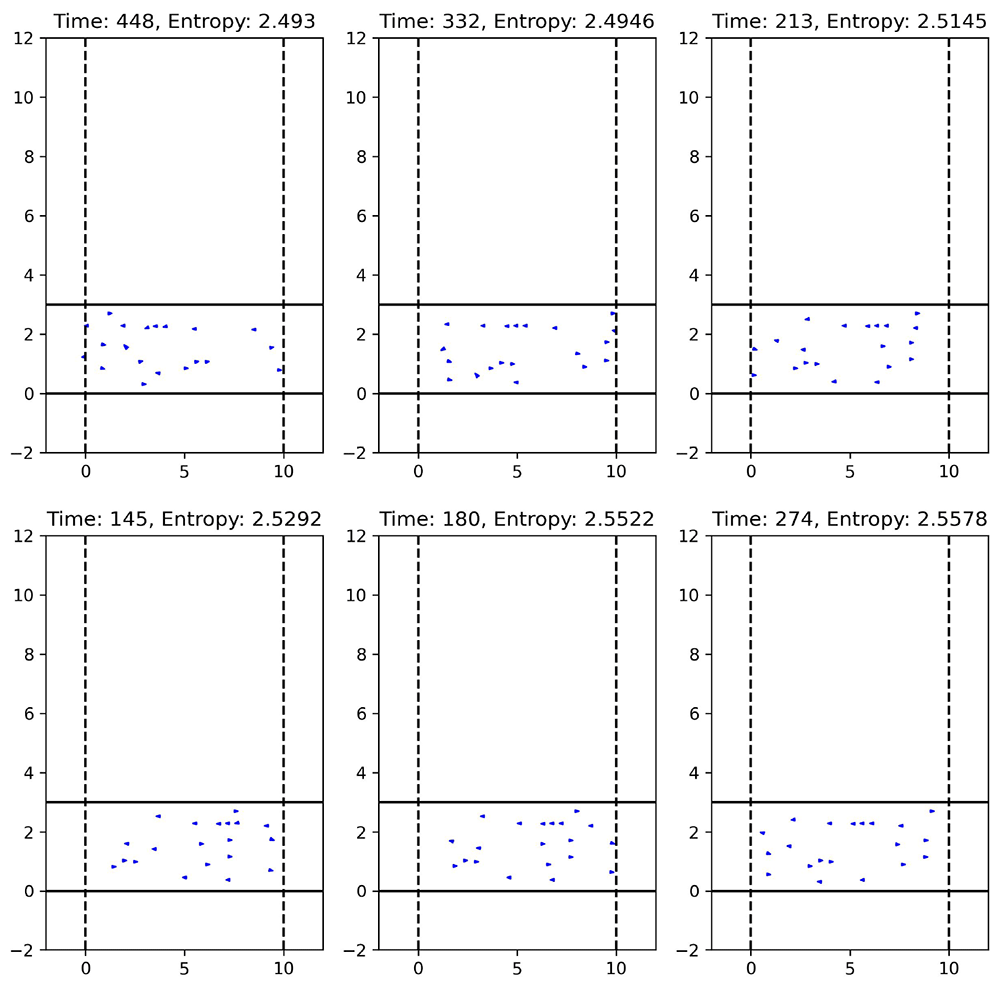
Figure 35. Time steps with high entropy of a simulation run with 20 agents, where agents followed the HL behavior.

Lower entropy means that intervals are more unevenly distributed and suggests less dispersion of the agents, so that some agents are somewhat clustered together in one area of space, and others are further apart in another area, leaving areas somewhat empty. In Figure 36, we show the point clouds corresponding to local minima with a minimum distance of 20 time steps between them, as consecutive minima may not indicate significant changes.

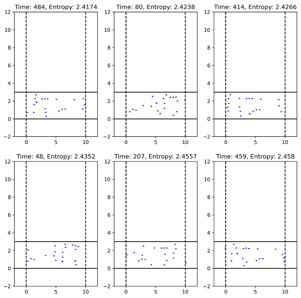
Figure 36. Time steps with low entropy of a simulation run with 20 agents, where agents followed the HL behavior.

Summing up, a specific time step in a simulation run with higher entropy indicates greater dispersion among the agents, that is, a more uniform distribution of the agents across the space, with fewer clusters and fewer empty or sparsely populated regions. Conversely, lower entropy suggests less dispersion of the agents, with agents more likely to concentrate in specific areas, forming clusters and leaving other regions empty.

Similarly, we executed a single simulation run with 20 agents, where each agent followed the ORCA navigation behavior. This simulation run consists of 500 time steps with a time increment of 0.1 seconds between each step, lasting a total of 50 seconds. We obtain similar results for this behavior as before. We explain the distribution of agents in space using persistent entropy: higher entropy suggests a greater dispersion among the agents. Conversely, lower entropy suggests less dispersion. See Figure 37 for the time steps corresponding to the different deciles of the entropy time series, where we illustrate how persistent entropy reflects the spatial distribution of agents. Figure 38 presents the time series of the persistent entropy time series obtained using ORCA behavior. In this case, entropy fluctuates between 2.325 and 2.5, showing a general downward trend over time. This indicates that the agents tend to cluster more over time, leaving some areas of space emptier.

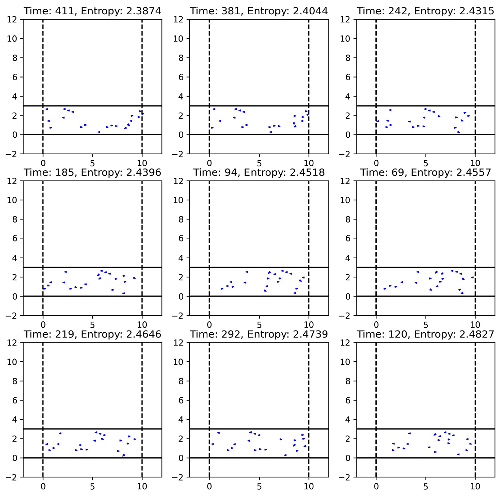
Figure 37. Time step of the different deciles of the persistent entropy time series for a simulation run with 20 agents, where agents followed the ORCA behavior.

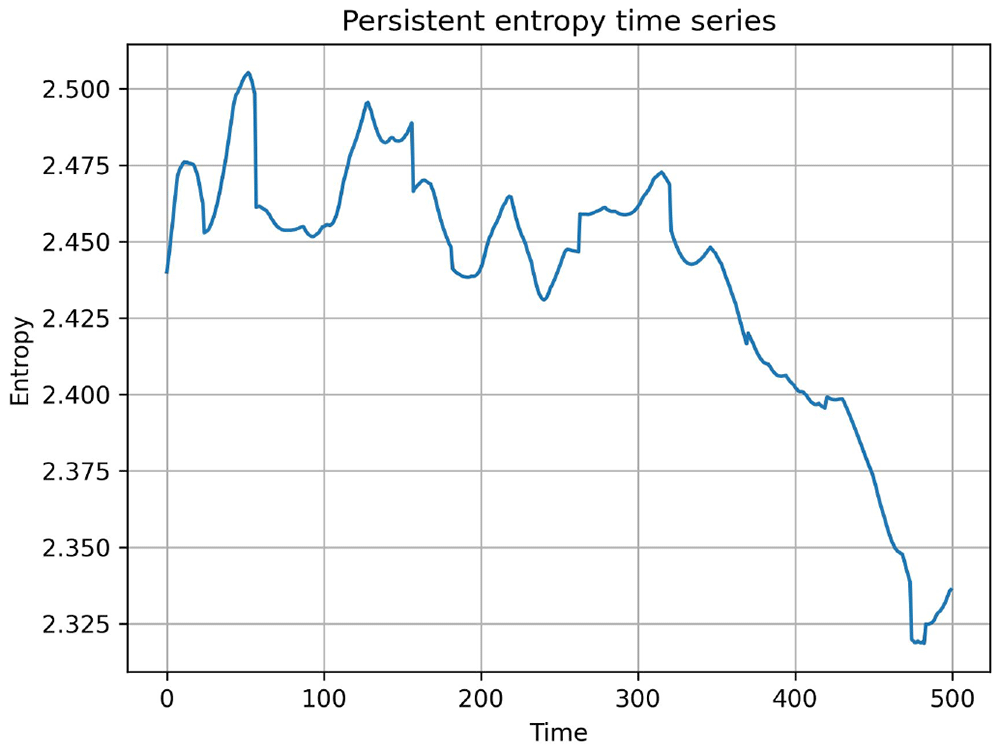
Figure 38. Persistent entropy time series of a simulation run with the agents following the ORCA behavior.

Figure 34 and Figure 38 show the persistent entropy time series for a simulation run following the HL and ORCA behaviors, respectively. As we can observe, the two series do not follow a similar pattern or shape. While HL persistent entropy time series shows an initial dispersion pattern followed by moderate clustering, ORCA persistent entropy time series tends towards more pronounced clustering over time.

Secondly, we executed N = 10 simulation runs with 20 agents, where agents followed the same behavior (HL or ORCA). Each simulation run consisted of 3000 time steps with a time increment of 0.1 seconds between each step, in a total duration of 300 seconds. We aimed to compare both behaviors through the persistent entropy time series. The safety_margin parameter was not fixed, but uniformly distributed between 0 and 0.5. The 10 simulation runs for each behavior were conducted with identical parameters, including the same safety_margin. We can see the persistent entropy time series obtained for the simulation runs using the HL and the ORCA behavior in Figure 39 and Figure 40, respectively. Several differences were noted:

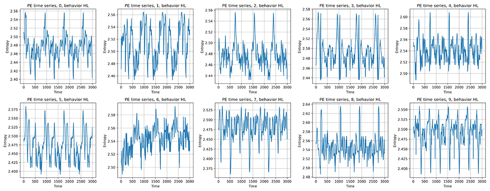
Figure 39. Persistent entropy time series for different simulation runs with the agents following the HL behavior.

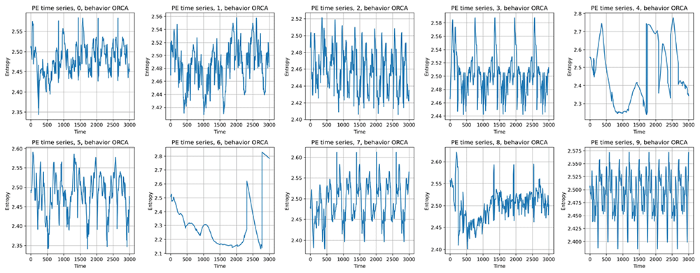
Figure 40. Persistent entropy time series for different simulation runs with the agents following the ORCA behavior.

Oscillation patterns: The persistent entropy time series for the HL behavior exhibit smooth and regular oscillations. The amplitude of these oscillations remains consistent over time, indicating a stable and predictable behavior of the system. In contrast, the time series for ORCA exhibit more irregular oscillations with greater variability in amplitude. There are more pronounced and less predictable fluctuations, suggesting a more unstable behavior.
Persistent entropy stability: The persistent entropy in HL simulation runs remains within a narrow range of values, showing little variation between different simulation runs. This denotes high stability and consistency in the agent’s behavior under this mode. On the other hand, ORCA simulation runs exhibit greater dispersion in persistent entropy values. Some experiments show significant variations, which indicate that the behavior is more sensitive to initial conditions or changes in parameter values, such as safety_margin.
Transitions and abrupt changes: Transitions between time steps with different persistent entropy values are gradual and smooth, reflecting continuous and controlled adaptation of the system in the HL simulation runs. In ORCA simulation runs, there are more abrupt and sudden changes in the persistent entropy time series. These rapid transitions indicate more reactive responses or fluctuations in the agent’s behavior.
Consistency between simulation runs: There is a high similarity between the persistent entropy time series of different simulation runs for the HL behavior. The patterns are consistent, suggesting that the behavior is robust and less prone to random variations. On the other hand, ORCA simulation runs show greater diversity in the persistent entropy time series. Some time series differ significantly from others, which implies that this behavior is more complex or influenced by multiple factors.
General trends: In the HL simulation runs, the persistent entropy time series maintain a relatively constant trend without marked deviations, which may be associated with balanced and stable behavior. In contrast, the persistent entropy time series computed from the ORCA simulation runs exhibit upward or downward trends during certain time intervals, indicating possible changes in the system’s state or the agents’ activity.

In summary, persistent entropy time series computed from simulation runs following HL behavior tend to exhibit greater stability, consistency, and regularity. In contrast, persistent entropy time series computed from simulation runs following ORCA behavior display greater variability, characterized by more irregular oscillations and abrupt transitions. These differences suggest that agents following HL behavior operate more predictably and stably, whereas those following ORCA behavior exhibit more complex dynamics and may be more adaptive or sensitive to changes in the environment.

Thirdly, we performed an analysis comparing specific statistical properties of the persistent entropy time series for the two behaviors, using boxplots and hypothesis testing, specifically the Mann–Whitney test. The boxplots are used to visualize the distribution of different metrics (means, medians, standard deviations, interquartile range) between the two types of simulation runs (HL and ORCA), while the Mann-Whitney test is performed to determine whether the observed differences between the two types of simulation runs are statistically significant. See Figure 41.

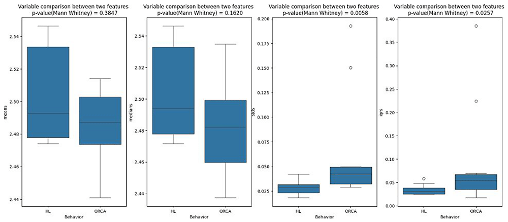
Figure 41. Boxplot analysis between HL and ORCA behaviors for the Corridor scenario.

Out of the four analyses performed, standard deviation and interquartile range show significant differences between the HL and ORCA behaviors, while the comparisons of means and medians do not present significant differences. This suggests that although the central tendency measures are similar for both behaviors, the dispersion measures differ.

Lastly, we executed N = 100 simulation runs for each behavior (HL and ORCA), with 40 agents. Each simulation run consists of 1000 time steps with 0.1 seconds between each step, lasting a total of 100 seconds, with safety_margin parameter not fixed, but uniformly distributed between 0 and 0.1. We aimed to analyze the relationship between the time series through statistical metrics (mean, median, standard deviation, skewness, and interquartile range) with collisions and simulation efficacy (which is highly related to deadlocks). First, we focus on simulation runs in which the agents follow the HL behavior and then on those in which the agents follow the ORCA behavior.

Regarding HL simulation runs, the analysis suggests that medians, standard deviations, and interquartile ranges have significant correlations with simulation efficacy. While medians are slightly positively correlated (ρ = 0.35, p-value= 0.0004), standard deviations (ρ = −0.89, p-value= 1.95 × e⁻³⁴) and interquartile range (ρ = −0.83, p-value= 6.42 × e⁻²⁷) are strongly negatively correlated with simulation efficacy, meaning that simulation runs with lower standard deviations and interquartile range about the persistent entropy time series will have a higher efficacy. Means and skewness do not show a significant relationship with efficacy. See, in Figure 42, the scatter plots between these statistical metrics of the persistent entropy time series and simulation efficacy, where we show the relationships we have discussed. Also, some examples of persistent entropy time series of simulation runs with lower efficacy are shown in Figure 43, and higher efficacy in Figure 44.

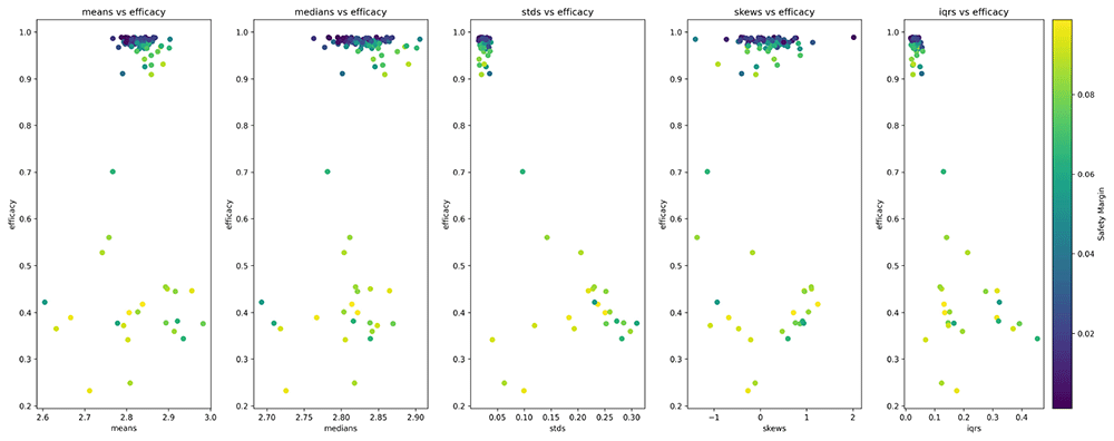
Figure 42. Scatter plots between statistical metrics of the persistent entropy time series and simulation efficacy for the HL behavior.

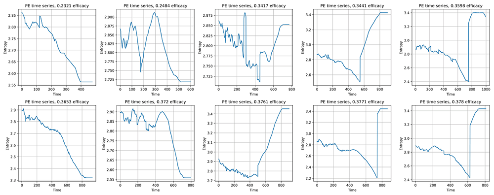
Figure 43. Persistent entropy time series of Navground simulation runs with less efficacy for the HL behavior.

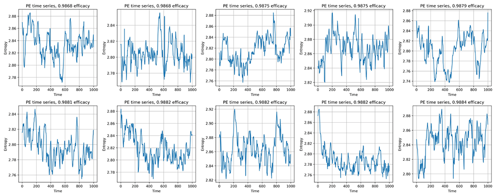
Figure 44. Persistent entropy time series of Navground simulation runs with greater efficacy for the HL behavior.

Different patterns can be observed, particularly in the time series of simulation runs with low efficacy, which show very pronounced drops or increases in entropy until they stabilize completely. This indicates that all the agents are likely in a deadlock state, with no movement occurring. In contrast, simulation runs with high efficacy exhibit the constant oscillations and periodicity that we have seen in previous graphs. On the other hand, if we make a similar analysis with collisions, we do not have any significant correlation between these metrics and collisions.

Regarding ORCA simulation runs, the analysis also suggests that standard deviations and interquartile ranges have significant negative correlations with simulation efficacy, meaning that simulation runs with lower standard deviations and interquartile ranges in reference to the persistent entropy time series will have a higher efficacy. See in Figure 45, the scatter plots between these statistical metrics of the persistent entropy time series and simulation efficacy, where the relationships we have discussed previously are shown. In the same way, the differences between persistent entropy time series of simulation runs with lower efficacy and higher efficacy persist for ORCA behavior.

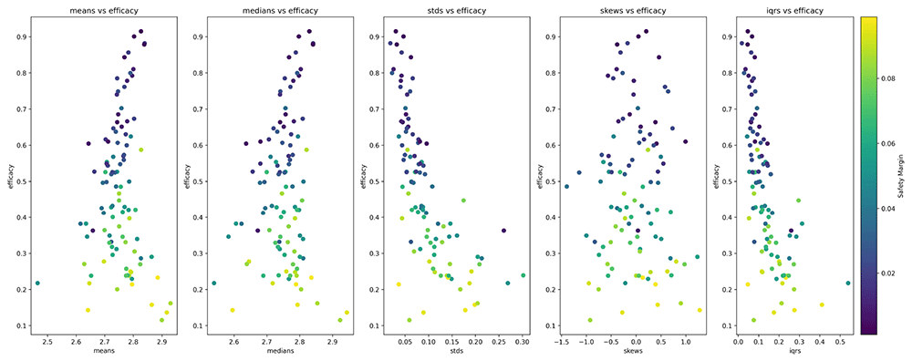
Figure 45. Scatter plots between statistical metrics of the persistent entropy time series and simulation efficacy for the ORCA behavior.

In addition, in ORCA simulation runs, the analysis suggests that while standard deviations and interquartile range are slightly positively correlated with simulation efficacy, means and medians are negatively correlated with simulation efficacy, meaning that simulation runs with lower means and medians in reference to the persistent entropy time series will be more efficient. Skewness does not show a significant relationship with efficiency. See in Figure 46, the scatter plots between these statistical metrics for the persistent entropy time series and safety.

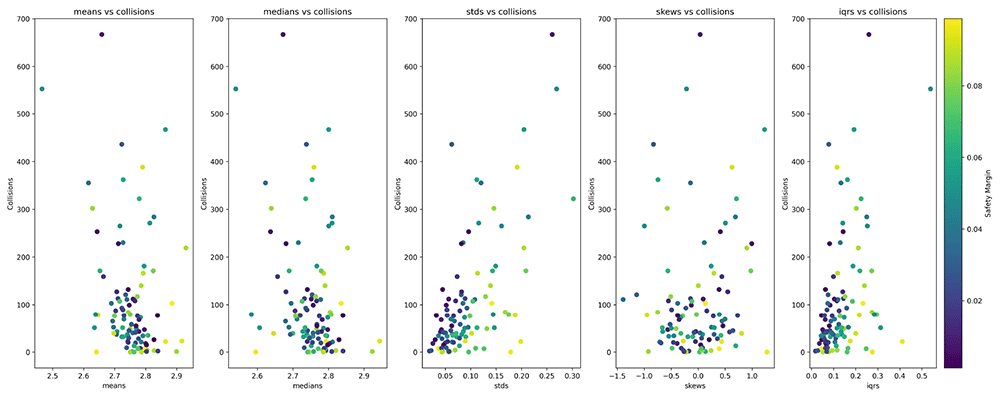
Figure 46. Scatter plots between statistical metrics of the persistent entropy time series and collisions for the ORCA behavior.

Cross scenario. For this scenario, we have limited ourselves to commenting and explaining the results obtained, without adding figures, in order not to extend the document any further.

First, we executed a single simulation run for each behavior, with 20 agents, where each agent followed the specific navigation behavior (ORCA or HL). This simulation run consists of 500 time steps with a time increment of 0.1 seconds between each step, lasting a total of 50 seconds.

As for the Corridor scenario, once again, a time step with a higher entropy indicates a greater dispersion among the agents in relation how they are distributed around the space, without agent clusters in certain areas and without empty areas or areas with few agents, being less likely to have empty areas and to form cluster of agents very grouped and another ones very far away, while a lower entropy indicates that less dispersion between the agents, being more likely to occupy specific regions of space and form clusters.

Regarding the study of the correlation between the persistent entropy changes between two consecutive time steps and the total distance traveled by the agents during these steps, we found a slightly significant correlation (ρ = 0.21, p-value= 3.2 × e⁻⁶ for ORCA and ρ = 0.15, p-value= 0.001 for HL), meaning that if there is a larger persistent entropy change in space due to the agents’ movement between two consecutive steps, the total distance traveled by the agents will be greater than in steps with lower or slight entropy changes, where the agents move less. This slightly positive significant correlation indicates a weak positive relationship between these two variables. Additionally, it is worth noting that between two consecutive time steps, the total distance traveled by the agents is greater for ORCA than for HL in the Corridor scenario, while the opposite occurs in the Cross scenario. Comparing different simulation runs in this type of scenario with HL and ORCA behaviors, they exhibit notable differences in several aspects. In terms of general trends, the HL simulation runs show persistent entropy values that remain within a relatively high range, whereas several ORCA simulation runs show a more pronounced downward trend, suggesting that the average entropy may be decreasing over time. Regarding variability and oscillations, HL simulation runs exhibit significant fluctuations but within a more constrained range, while for ORCA simulation runs, although oscillations are also present, some time series show a more pronounced decrease with lower minimum values.

The range of entropy values also differs between the two behaviors. In the HL simulation runs, the values appear to be concentrated between 2.55 and 2.75. In contrast, in the ORCA simulation runs, a wider range is observed, approximately between 2.3 and 2.8, indicating greater variability. Additionally, the long-term behavior shows that in the HL simulation runs, entropy remains relatively stable, fluctuating without a clear trend, while in the ORCA simulation runs, some time series exhibit a more evident decline, suggesting that this behavior tends to become more predictable over time.

In conclusion, the ORCA simulation runs display greater variability and a tendency toward persistent entropy reduction in some series, while in the HL simulation runs, entropy remains more stable and higher. This could indicate that the ORCA behavior generates a more structured or less chaotic pattern over time compared to the HL behaviour.

An analysis is also conducted that involves comparing certain statistical variables for the two behaviors using boxplots and hypothesis testing, specifically the Mann-Whitney test. In the boxplots that correspond to the means and medians of the time series, HL behavior shows slightly higher values compared to ORCA behavior, although the distributions overlap considerably. The p-value of 0.1859 indicates that this difference is not statistically significant, suggesting that the differences in mean and median entropy between the two behaviors are inconclusive. On the other hand, the boxplots representing standard deviation and interquartile range reveal more noticeable differences. In particular, ORCA behavior exhibits a higher standard deviation, indicating greater variability in entropy compared to HL behavior. The p-value of 0.0140 suggests that this difference is statistically significant. Additionally, kurtosis is also higher in ORCA behavior, meaning that its distribution has heavier tails or is more concentrated around certain values compared to HL behavior. The p-value of 0.0058 confirms that this difference is also significant.

In conclusion, while the mean and median entropy values do not show significant differences between HL and ORCA behaviors, the variability and distribution characteristics do. ORCA behavior exhibits greater dispersion and a more extreme distribution compared to HL behavior, supporting the idea that ORCA generates a more variable and less stable dynamic over time.

Lastly, we execute N = 100 simulation runs for each behavior (HL and ORCA), with 40 agents. Each simulation run consists of 1000 time steps with a time increment of 0.1 seconds between each step, lasting a total of 100 seconds. As we want to compare both behaviors through the persistent entropy time series for each simulation run, safety_margin parameter is not fixed, but uniformly distributed between 0 and 0.1. Regarding the HL simulation runs, the analysis suggests that the ranges of means and medians in the persistent entropy time series have a strong negative significant correlation with the number of collisions (ρ = −0.64 for the mean and the number of collisions, and ρ = −0.62 for the median and the number of collisions). This implies that simulation runs with lower mean or median persistent entropy are more likely to experience a higher number of collisions among agents. In contrast, standard deviation, skewness, and interquartile range do not show a significant relationship with the number of collisions.

Similarly, these variables exhibit the same relationship with simulation efficacy (ρ = −0.59 for the mean and the simulation efficacy, and ρ = −0.55 for the median and the simulation efficacy): the lower the mean or median persistent entropy, the higher the efficacy. In other words, a lower mean or median entropy value reduces the likelihood of deadlocks, as higher efficacy indicates that agents move at a speed close to the optimal one. This suggests that lower entropy states may correspond to more structured and coordinated agent movements, allowing for smoother navigation and fewer disruptions caused by congestion or erratic behavior.

The results obtained suggest that there is a strong, positive, and significant correlation between the mean and median time series with both the number of collisions (ρ = −0.57 for the mean and the number of collisions, and ρ = −0.57 for the median and the number of collisions) and simulation efficacy (ρ = −0.88 for the mean and the efficacy, and ρ = −0.88 for the median and the efficacy).

These aspects, which show differences between the behaviors in both scenarios, suggest that we could create a classifier that, using the time series of persistent entropy as input, could predict the type of behavior followed by the agents in the simulation run.

5.2.2 L2: Topology-based safety region construction for collision and deadlock avoidance. Using Navground, we generated a suitable dataset to study the safety of agents’ movement while avoiding collisions, deadlocks, and both of them, via probabilistic scaling and conformal prediction methods, with interpretation via rule-based classifiers. We executed N = 10000 simulation runs, each with 2000 time steps, with a time increment of 0.1 seconds. We considered a fleet of 20 agents. Each agent follows the HL behavior with the following parameters:

v_opt = 0.12 m/s
τ_rot = 0.5 s
σ sampled uniformly from [0.0 m, 0.1 m] for collision avoidance, and from [0.0 m, 0.5 m] for deadlock avoidance and safe and efficient simulation runs.
τ and η sampled uniformly from [0.0 s, 1.0 s]

The HL parameters σ, η and τ (see Table 2) have been sampled to generate simulation runs of all types, including safe, aggressive, cautious, or efficient simulation runs.

For each simulation run, we apply the methodology explained in Subsection 5.1, recording the following values:

x = (m e a n E n t r o p y, m e d i a n E n t r o p y, s t d E n t r o p y, ​ i q r E n t r o p y),

Then, we assigned a binary label y to each simulation run through the following criteria, depending on the avoidance event:

Safe simulation run (avoiding collision):
$y = {\begin{array}{l} + 1 & if number of collisions = 0, \\ - 1 & if number of collisions > 0. \end{array}$
Efficient simulation run (avoiding deadlocks):
$y = {\begin{array}{l} + 1 & if number of deadlocks = 0, \\ - 1 & if number of deadlocks > 0. \end{array}$
Compliant simulation run (avoiding both collision and deadlocks):
$y = {\begin{array}{l} + 1 & if number of collisions & deadlocks = 0, \\ - 1 & if number of collisions & deadlocks > 0. \end{array}$

Finally, we obtained there dataset $T_{nav}^{i}$ = {(x_j, y_j) | j = 1, . . . , N} for i = 1, 2, 3, corresponding to the three criteria, respectively.

A first visual inspection of how classes are distributed in the datasets is useful to understand the nontrivial nature of the problem. In Figure 47a, Figure 47b and Figure 47c, the relationships among the four entropy-based metrics — mean entropy, median entropy, standard deviation of entropy, and interquartile range of entropy — are visualized for the three binary classifications: collision avoidance, deadlock avoidance, and compliant simulation runs. Each plot displays pairwise scatterplots, overlaid with kernel density estimation (KDE) curves along the diagonals to depict distributions for each class. Simulation runs with lower meanEntropy and medianEntropy values are more closely associated with collisions, indicating that decreased entropy could signal potential collisions between agents. Higher values of meanEntropy and medianEntropy are more closely associated with the “deadlock” class, indicating that increased persistent entropy in the system could signal a potential deadlock situation. In this way, we can observe how safe and efficient simulation runs, without collisions or deadlocks, have relatively stable values for mean entropy and median entropy.

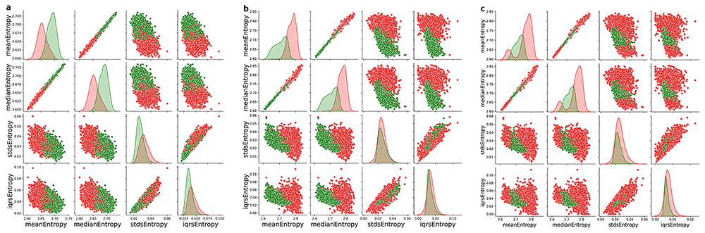
Figure 47. Pairwise class distributions of the features in $T_{nav}^{i}$ for i = 1, 2, 3.

(a) Safety: green = no collision, red = collision. (b) Efficiency: green = no deadlock, red = deadlock. (c) Compliance: green= no collision or deadlock.

Across all three classifications — safe, efficient, and compliant simulation runs — meanEntropy and medianEntropy stand out as the most informative features for distinguishing between classes. While stdEntropy and iqrsEntropy provide less individual discriminatory power, they may still offer complementary information when used in combination with the other metrics. These insights highlight the potential of persistent entropy-based metrics for identifying critical system states and suggest a strong basis for further model development and optimization.

Results. First, we compare training a rule-based model with the behavior parameters (as is done in 36) against training it with the topological features extracted with our methodology for collision avoidance. For that, we use SkopeRules¹⁰, which is a rule-based ML algorithm that learns interpretable and diversified rules for “scoping” a target class of interest, i.e., detecting samples from this class with high precision. In practical applications, the SkopeRules model has been applied to several safety-critical classification tasks, as well as anomaly detection problems or cluster description.

Table 3 highlights the superior performance of SkopeRules using topological features compared to using behavior parameters. The topological model achieves higher accuracy (84.6% vs. 83.6%), F1-score (84.6% vs. 81.9%), and true negative rate (81.3% vs. 72.5%) while significantly reducing the false positive rate (18.7% vs. 27.5%). Although its true positive rate (87.1% vs. 92.0%) is slightly lower, and the false negative rate (12.9% vs. 8.0%) is higher, these trade-offs are outweighed by its improved balance across metrics. Remember that the positive class is the non-collision class (+1).

Table 3. Performance comparison between the adopted rule-based models.

The first column refers to the input features. The second column reports the number of generated rules. The other columns refer to the following metrics (expressed in %): accuracy (ACC), F1-score (F1), true positive rate (TPR), false positive rate (FPR), false negative rate (FNR), true negative rate (TNR).

	# of rules	ACC	F1	TPR	FPR	FNR	TNR
SkopeRules-behavior parameters	8	83.6	81.9	92.0	27.5	8.0	72.5
SkopeRules-topological features	20	84.6	84.6	87.1	18.7	12.9	81.3

The use of 20 rules, compared to 8 for behavior parameters, suggests the topological model captures more complex relationships, enhancing its robustness. Models with fewer rules have the advantage of being more interpretable, but the richest ones may generate more fine-grained rules with better discriminative ability. Overall, topological features provide a more discriminative representation, making this model preferable for scenarios prioritizing accuracy and minimizing false positives.

Also, we compared the safety regions generated using these two types of input features. Specifically, we considered a Gaussian kernel SVM, with a sigma set to 0.5, with a regularization parameter set to 0.3, and a weighting of 0.5. With this base model, before any error control, we achieved the following performance: 78.2% accuracy, 80.6% F1-score, 82.8% TPR, 72.7% TNR, 27.3% FPR, 17.2% FNR using behavior parameters as input and 85% accuracy, 88.1% F1-score, 91.6% TPR, 75% TNR, 25% FPR, 8.4% FNR using topological features as input.

Topological features consistently show better performance than behavior parameters across all metrics, both in baseline classification and in safety region generation. Among the methods for generating safety regions (see Table 4), conformal prediction demonstrates superior accuracy and F1-scores, particularly with topological features, making it the preferred approach for ensuring robust safety guarantees.

Table 4. Performance comparison between the adopted techniques for finding safety regions at ϵ = 0.1.

The first column refers to the input features used for training the classification models, the second column refers to the adopted techniques for finding safety regions (probabilistic scaling - PS, and conformal prediction - CP), and the third one reports the optimal scaling parameter. The other columns refer to the following metrics (expressed in %): accuracy (ACC), F1-score (F1), true positive rate (TPR), false positive rate (FPR), false negative rate (FNR), true negative rate (TNR).

	Method	ρ_ϵ	ACC	F1	TPR	FPR	FNR	TNR
Behavior parameters	PS	0.49	77.9	77	67.8	9.9	32.1	90.1
Behavior parameters	CP	0.44	78.5	77.8	69	10.1	31	89.9
Topological Features	PS	0.42	79.8	81.6	74.3	11.9	25.7	88.1
Topological Features	CP	0.21	83.7	86.2	84.1	16.9	15.9	83.1

Now, we derive interpretable approximations for both regions in the form of decision rules. Local rule extraction via Anchors was performed on a set of steps labeled as +1 by the adjustable classifiers and sampled at a small distance d ≤ 0.05 from their border.

The results in Table 5 demonstrate the advantages of using topological features over behavior parameters in the context of local rule extraction with Anchors. Notably, the number of generated rules (anchors) is significantly reduced when using topological features—only 2 rules compared to 5 rules for behavior parameters:

Table 5. Performance comparison between the rules obtained using Anchors from the obtained adjustable classifiers (SVM).

The first column refers to the input features used for training the adjustable classifiers, the second refers to the adopted techniques for finding safety regions, and the third column reports the number of generated rules (anchors). Coverage and error percentages are reported for the logical union of the anchors being tested with respect to the labels assigned via PS and CP (Method labels column), and the real labels (Ground truth column). Coverage measures the proportion of correctly classified positive samples, and error represents the proportion of false positives, in the total predictions. Probabilistic scaling is denoted as PS, and conformal prediction is denoted as CP.

			Method labels		Ground truth
	Method	# of anchors	Coverage	Error	Coverage	Error
Behavior parameters	PS	5	86	36	73	29
Behavior parameters	CP	5	85	35	73	29
Topological features	PS	2	79	0	69	9
Topological features	CP	2	100	30	100	26

Topological features—rules: meanEntropy > 2.68 and medianEntropy > 2.68 for PS method, and meanEntropy > 2.66 and medianEntropy > 2.65 for CP method. Entropy above these values refers to simulation runs free of collision situations.
Behavior parameters -rules: the same 5 rules for both methods: η > 0.75, τ ≤ 0.5, τ ≤ 0.25, τ ≤ 0.76 and σ > 0.08.

This reduction highlights a key advantage: the rules obtained with topological features are simpler, more concise, and easier to interpret, which enhances their applicability in decision-making tasks. In addition, for topological features, the error rates are significantly lower. For step, under probabilistic scaling (PS), the error drops to 9%, compared to 29% with behavior parameters. Even with conformal prediction (CP), the error decreases to 26%, while achieving a perfect 100% coverage. Despite having fewer rules, topological features maintain competitive or superior coverage compared to behavior parameters.

These findings emphasize that topological features not only simplify the decision rules by reducing their number but also improve their accuracy and reliability, making them a more effective and interpretable choice for defining local decision regions.

Once we have verified that the proposed methodology achieves better results for differentiating between safe (no agent collisions) and non-safe simulation runs, we proceed to extend its use to the case of distinguishing between efficient (no deadlocks) and non-efficient simulation runs. We follow the same steps as above, but this time we do not compare the results/performance with those obtained using behavior parameters (σ, η and τ).

Using the SkopeRules method and topological features to classify non-efficient simulation runs (i.e., with deadlocks) versus efficient simulation runs (i.e., without them), we derive a total of 18 rules, achieving highly positive performance: 89% accuracy, 88.5% F1-score, 93% TPR, and 84% TNR. This demonstrates that these features achieve even better performance for deadlock avoidance than for collision avoidance when using SkopeRules.

Next, we generate the safety regions using these features in the same manner as before. We considered a Gaussian kernel SVM, with a sigma set to 0.5, a regularization parameter set to 0.3, and a weighting of 0.5. With this base model, prior to any error control, we achieve the following performance: 86% accuracy, 82.3% F1-score, 74.7% TPR, 94.7% TNR. Using PS method we achieve the following performance: ρ_ε equal to -0.12, 87.2% accuracy, 84.6% F1-score, 80.1% TPR, 92.7% TNR; and using the CP method, we achieve the following performance: ρ_ε equal to 0.17, 83.6% accuracy, 77.9% F1-score, 66% TPR, 97.3% TNR.

Again, local rule extraction via Anchors was performed on a set of steps labeled as +1 by the adjustable classifiers and sampled at a small distance d ≤ 0.05 from their border. The number of generated rules (anchors) is 2 (same for both methods: meanEntropy ≤ 2.75 and medianEntropy ≤ 2.75. Persistent entropy below these values refers to simulation runs free of deadlock situations, so again, the rules obtained are very simple and easy to interpret. We evaluate the logical union of the anchors being tested concerning the labels assigned via the method used, and the real labels, obtaining the following results:

91% coverage and 21% error for ground truth labels, and 100% coverage and 22% for method labels for PS method.
91% coverage and 21% error for ground truth labels, and 100% coverage and 39% for method labels for PS method.

We can see how, with the PS method, we obtain a better performance in terms of error and, with the CS method, a better performance in terms of covering (as for collision avoidance using topological features), although the rules are the same, obviously obtaining the same performance for the real labels. Considering the non-trivial nature of the problem and of approximating a complex SVM shape via hyper-rectangular shapes (rules) while keeping the error bound as low as possible, we consider our results as a promising compromise between safety and transparency.

Thus, if we focus on distinguishing between compliant (safe and efficient) simulation runs (i.e., free of collisions and deadlocks) and non-compliant simulation runs, we obtain very simple rules for both methods:

2.68 ≤ meanEntropy ≤ 2.75 and 2.68 ≤ medianEntropy ≤ 2.75 for the PS method.
2.66 ≤ meanEntropy ≤ 2.75 and 2.65 ≤ medianEntropy ≤ 2.75 for the CP method.

In summary, our results highlight the advantages of using topological features in rule-based explanations and the generation of safety regions for classification. First, for differentiating between safe and unsafe simulation runs, we achieve better results compared to not using these topological features. The results were even more favorable for distinguishing between efficient and non-efficient simulation runs, ultimately yielding a very simple rule for differentiating between compliant and non-compliant simulation runs. These findings confirm the suitability of topological features for enhancing transparency and reliability in classification and safety detection tasks.

Finally, since these rules are a posteriori to the simulation runs — meaning that we need to have the complete simulation run and calculate these topological features to determine whether it falls within the safety margins defined by the obtained rules — it would be interesting to explore how to define the simulation parameters a priori so that the resulting runs exhibit a safe persistent entropy value, that is, one that falls within the range identified as safe by the rules.

The results presented in Figure 48 and Figure 49 analyze the relationship between three parameters (σ, η and τ) and the classification of simulation runs into safety or non-safety, based on a posteriori safety rule evaluation. The goal is to understand how these parameters influence the safety classification and derive insights that could help define simulation parameters a priori to ensure safety.

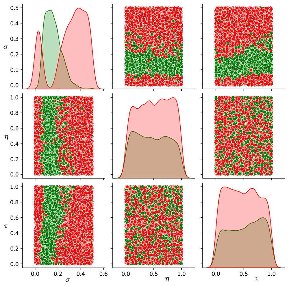
Figure 48. Pairwise class distributions between simulation parameters (σ, η and τ) and the compliance classification (green color refers to “safe” label, and red color to “non-safe” label) based on the a posteriori safety rule (using the PS method rules, since it has a lower error for both collision and deadlock avoidance than the CP method rule).

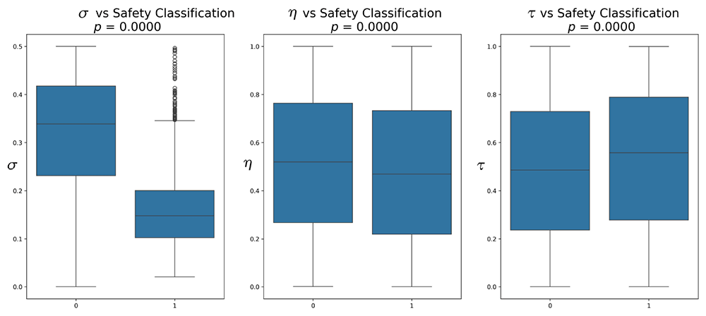
Figure 49. Statistical comparison using boxplots for the parameters σ, η and τ, and the safety classification (0: unsafe, 1: safe), evaluated based on the a posteriori safety rule.

The p-values fromthe Mann-Whitney test indicate statistically significant differences between the safety categories (p ≤ 0.05).

The findings suggest that σ is the most influential parameter for determining whether a simulation run satisfies the safety rule. Specifically, setting lower values of σ a priori increases the likelihood of achieving a safe outcome. Setting σ within a low range (0.1–0.2) a priori may increase the likelihood of meeting the safety rule. While η and τ also show statistically significant relationships with safety, their influence appears more subtle and may act as secondary contributors. To optimize simulation parameters for safety adherence, prioritizing low σ values, with careful consideration of η and τ, is recommended. This analysis provides a robust foundation for a priori parameter selection in simulation runs, enabling a more systematic and predictive approach to ensuring safety compliance.

An important aspect to consider is that these ranges are sensitive to the number of agents and the scenario, meaning these results cannot be generalized to all cases. Additionally, it is necessary to assess whether it is also sensitive to the type of behavior used.

6 Navigation behavior characterization with matching diagrams

In this section, we develop a novel data analysis method based on matching diagrams, designed to track the evolution of clusters from Navground simulation runs. In a nutshell, the proposed method tracks the evolution of groups of autonomous agents, which gives a characterization of the fleet behavior. Specifically, our method analyses the evolution of agents’ states to characterize different Navground behaviors.

The intuitive idea that inspires our approach is that order or chaos in autonomous fleet behavior can be measured by the formation of groups of agents, see 37. As persistent homology quantifies the importance of clusters in a metric space, it is a natural signature for measuring such order or chaotic behavior. Our contribution could also be used in other applications from science or industry, where the aim is to characterize the movement of agents or particles.

We have divided the section into two subsections depending on the input data and the similarity measure used to compute the matching diagrams. In 6.1, we use the agents’ pose and twist as the input data and the ambient Euclidean metric as the similarity measure, whereas in 6.2 we use times series obtained from the agents’ trajectories as the input data and the DTW distance as the similarity measure.

6.1 Euclidean metric as the similarity measure for behavior characterization with matching diagrams

We compare pairs of time steps to detect differences in the configuration of agents. We have developed a new data analysis technique based on 0-dimensional persistent homology.

Recall that 0-dimensional persistent homology gives a measure of clusters in a point cloud. To compare agent positions between pairs of time steps, we use the block function, which we introduced in Subsection 2.6. Our proposed methodology is specifically designed to track the formation of groups in a simulation run along the time steps. In addition, our method is versatile and can be used in a wide variety of contexts.

We proceed now to explain our method overall and show the experiments conducted on Navground.

6.1.1 Methodology. As mentioned in Subsection 3.2, there is an amount of data that one obtains after running a simulation, which depends on the simulation length, number of agents, among other factors. Our proposed pipeline is divided into four steps, whose input is the data saved from running a simulation.

1. Construct a sequence of similarity matrices ${(L_{t}, R_{t})}_{t = 1}^{M},$ for all integers 1 ≤ t ≤ M, from the pairs of time steps (X_t, Y_t).
2. Compute the matching diagrams D(X_t, Y_t) for all 1 ≤ t ≤ M,
3. Vectorize the sequence ${D (X_{t}, Y_{t})}_{t = 1}^{M},$ and
4. Perform data analysis on the output vectors.

Next, we describe in detail the workflow, which is depicted in Figure 50.

Figure 50. Pipeline of the proposed methodology.

1. Navground simulation data. Let us now detail how to obtain a pair of matrices (L, R) from the Navground output.

To start, for a time value t, the output Navground data for the i-th agent, 1 ≤ i ≤ N, consists of the agent’s poses and twists $x_{t}^{i}$ ∈ ℝ⁶, given as a tuple (x, y, α, v_x, v_y, v_α).

Now, we consider pairs of sequences of time values $A_{t} = (a_{1}^{t} < a_{2}^{t} < \cdot \cdot \cdot < a_{T}^{t})$ and $B_{t} : = (b_{1}^{t} < b_{2}^{t} < \cdot \cdot \cdot < b_{T}^{t}),$ with 1 ≤ t ≤ M.

Next, for the i-th agent, 1 ≤ i ≤ N, and for each t, 1 ≤ t ≤ M, there is a pair of vectors of simulation coordinates $x_{A_{t}}^{i} = (x_{a_{1}^{t}}^{i}, x_{a_{2}^{t}}^{i}, ..., x_{a_{T}^{t}}^{i})$ ∈ ℝ^6T and $x_{B_{t}}^{i} = (x_{b_{1}^{t}}^{i}, x_{b_{2}^{t}}^{i}, ..., x_{b_{T}^{t}}^{i})$ ∈ ℝ^6T. This leads to the sets $X^{t} = {x_{A_{t}}^{i}}_{i = 1}^{N}$ and $Y^{t} = {x_{B_{t}}^{i}}_{i = 1}^{N} .$ Next, we obtain the similarity matrices L_t and R_t by considering the ambient Euclidean metric, from which we construct the sequence ${(L_{t}, R_{t})}_{t = 1}^{M} .$

Notice that one needs to specify a few parameters, which we describe next:

the step shift ϵ, which is the difference $b_{1}^{t}$ − $a_{1}^{t}$ , which is constant along 1 ≤ t ≤ M, and where $a_{1}^{t}$ < $b_{1}^{t}$ holds for all 1 ≤ t ≤ M,
the initial step list, which is a list of evenly spaced values over which $a_{1}^{t}$ ranges,
the embedding length which is the length of sequences A_t and B_t; that is, the integer T,
the time delay δ, which is the difference $a_{j + 1}^{t} - a_{j}^{t} = b_{j + 1}^{t} - b_{j}^{t}$ which remains constant along 1 ≤ j < T and 1 ≤ t ≤ M,
the similarity measure; in this case, we consider the ambient Euclidean metric.

For example, suppose that we have M = 10. We take as step shift ϵ = 30, the initial step list equal to {1, 6, 11, . . . , 51}, the embedding length T = 3 and the time delay δ = 5. This leads to two sequences of time values A_t = (t, t + 5, t + 10) and B_t = (t + 30, t + 35, t + 40) parametrized by t ∈ {1, 6, 11, . . . , 51}. We then obtain a sequence of matrices ${(L_{t}, R_{t})}_{t = 1}^{10}$ by using an appropriate notion of similarity.

Now, notice that some scaling might be necessary to avoid a feature dominating over the others. We perform such scaling to give more or less importance to velocities. More precisely, an output Navground data $x_{t}^{i}$ ∈ ℝ⁶ for the i-th agent, 1 ≤ i ≤ N, is given as a tuple (x, y, α, v_x, v_y, v_α). It might be replaced by the tuple (x, y, α, wv_x, wv_y, wv_α) for some weight w > 0. In addition, we also discard some of the features, as for example, considering X^t and Y^t to consist only of the agents’ positions. An example of two time steps using Navground on the CrossTorus scenario is depicted in Figure 51.

Figure 51. Twelve agents moving on the CrossTorus scenario following the ORCA behavior.

The figure shows their positions at two time steps, connected by lines. In particular, notice that boundaries are periodic both horizontally and vertically.

2. Computation of the matching diagrams. Next, we take a list of pairs of time steps s(i) < t(i) with i = 1, . . . , M, and compute the matching diagrams $D = {D_{i} = D (X_{s (i)}, X_{t (i)})}_{i = 1}^{M}$ , as explained in Subsection 2.6. They satisfy that if N is the number of agents, then each matching diagram contains N − 1 points.

Consider the example depicted in Figure 51. We computed the corresponding matching diagram for some time step (dsee Figure 52). We considered matching diagrams for weights equal to w = 1 and w = 1.8 respectively, as well as step shifts equal to 10 and 30 respectively. Here, in our case N − 1 = 11. Notice that the matching diagrams change significantly by giving different weights and step shifts. In Figure 53, we superposed matching diagrams across time, considering the initial steps list.

Figure 52. Matching diagrams for weights taking values 1 and 3 and for steps shifts (epsilon) equal to 10 and 30 steps respectively.

Figure 53. Superposed matching diagrams ranging over the initial time steps.

Notice that the first two diagrams have a smaller scale than the others.

Example 4. In this example, we consider a simulation run on the Cross scenario. In particular, we take two pairs of time steps starting at 150 and 153 respectively, which we depict on the left of Figure 54. For each pair of time steps, we compute their respective matching diagrams and plot them on the right of Figure 54. We can see that the resulting matching diagrams remain stable. Furthermore, we can also see that the bijection from Theorem 1 holds.

Figure 54. Depiction of two time steps on the CrossTorus scenario at initial step 150 (left) and 153 (middle).

On the right, we depict their corresponding persistence diagrams, using red and blue colors respectively.

3. Vectorizations for matching diagrams. Once we have computed the matching diagrams, we vectorize 𝒟. We consider three possible ways for vectorization.

Our point of departure is a sequence of matching diagrams $D = {D_{t}}_{t = 1}^{M}$ which we vectorize to perform further data analysis. We consider three vectorizations: means of persistence images, persistence divergence images, and absolute persistence divergence. Next, we describe them in further detail.

1. Mean persistence images consists of a single persistence image, which results from computing the mean across several persistence images in a single simulation run. Specifically, we compute the persistence image ℐ(𝒟_t) of each matching diagram 𝒟_t for all t = 1, . . . , M; where we recall that persistence images are briefly described within Subsection 2.7. In particular, we consider persistence images with a constant weight equal to 1. Then, we consider the sum ℐ = (1/M) $\sum_{t = 1}^{M} I (D_{t})$ and call it the mean persistence image of 𝒟. For example, following this rule, we computed the vectorizations for the diagrams depicted in Figure 53, obtaining the resulting images in Figure 55. Notice that in these images, higher values occur around the middle horizontal line, which corresponds to the diagonal from matching diagrams.
2. Divergence image is a single image that summarizes the points that are far from the diagonal across time. Specifically, for each matching diagram 𝒟_t, we compute its divergence vector $V_{t} = {(b_{t}^{i} - a_{t}^{i})}_{t = 1}^{M - 1}$ which consists of the differences ranging over points in $D_{t} = {(a_{t}^{i}, b_{t}^{i})}_{i = 1}^{N - 1}$ for t = 1, . . . , M. We sort the entries in each divergence vector V_t from lower to higher values, and we store them as columns in a single matrix. The divergence image is the image depiction of such a matrix. Some example divergence images are depicted in Figure 56.
3. Absolute divergence: This vectorization is very similar to persistence images, but simpler. Specifically, we compute the sum $A_{i} = \sum_{i = 1}^{N - 1} | b_{t}^{i} - a_{t}^{i} |$ which adds up the absolute differences ranging over points in $D_{t} = {(a_{t}^{i}, b_{t}^{i})}_{i = 1}^{N - 1}$ for t = 1, . . . , M. This leads to a single vector ${(A_{t})}_{t = 1}^{M}$ which we call the absolute divergence. An example of such absolute divergence is depicted in Figure 57.
4. Data Analysis. The last step is to extract information from these vectorizations. For example, we can see that a change in the step shift significantly affects the output vectorization. See Figure 57.

Figure 55. Mean persistence images.

Figure 56. Persistence divergence images.

Figure 57. Absolute divergence.

6.1.2 Experiments. In our experiments, we compute matching diagrams throughout the simulation run and detect significant differences in the behaviors of the agent fleets.

We compare the results obtained using four behaviors — ORCA, HL, SFM, and HRVO — across three scenarios - Corridor, Cross, and CrossTorus. For all scenarios, we consider a few variables that are common across simulation runs. In particular, for each behavior, we run 15 simulations, each consisting of 500 steps with a time increment of 0.1 seconds. In each simulation, 12 agents move following some objective, which depends on the scenario. Each agent has a radius of 0.4 m and a safety margin of 0.1 m. The agents move with a maximum speed of 1.66 m/s and their optimal velocities are taken randomly, following a uniform distribution on the interval [1, 1.5]. As for matching diagram variables, we consider a step shift equal to 20 time steps, with an initial time step list equal to {1, 6, 11, . . . , 476} and a velocity weight of 1.

Experiments in the Corridor scenario. We consider simulation runs conducted in a corridor measuring 15 m in length and 3.5 m in width. For example, in Figure 58, the density of agents in the corridor is relatively high, and sometimes they move slowly because of the formation of groups, as can be seen on the HL time step depiction on the left. This is why the matching diagram related to the HL behavior contains all points around the diagonal, with small values being paired. On the other hand, for the time step considered, the simulation run on the ORCA behavior is moving more smoothly in some parts, while there are about three agents that seem to be stuck.

Figure 58. Movement of agents (left) and matching diagrams (right) for two time steps using HL and ORCA behaviors.

We computed the matching diagrams across the initial step list and depicted the superposition of the diagrams in Figure 59. As can be seen, the diagrams change significantly across behaviors.

Figure 59. Evolution of matching diagrams on the Corridor scenario across time, for the four behaviors considered.

To gauge how well the matching diagrams can detect behavior differences, we computed the mean persistence image on the various simulation runs. We projected them in two dimensions using the PCA projection, obtaining the projection depicted in the picture (a) in Figure 60. As we can see, the behaviors lie in different zones, with some overlap between the HL and the ORCA behaviors. We also perform the vectorizations of persistence divergence images and absolute divergences. We depict their PCA projections in the pictures (b) and (c) in Figure 60. We can see that the vectorization using persistence images is the one that performs best in a behavior classification task.

Figure 60. PCA of vectorizations of simulation runs on the Corridor scenario.

(a) PCA persistence images. (b) PCA persistence divergence. (c) PCA absolute divergence.

Experiments in the Cross scenario. We run simulations on the Cross scenario, with a side of 10 m. A depiction of two time steps, with their corresponding matching diagrams, is shown in Figure 61. We can see that the HL behavior tends to be more crowded than the ORCA behavior. This is reflected by the matching diagrams, where the points on the HL behavior are clustered around one portion of the diagonal, while the points from the ORCA matching diagram are more dispersed. Besides, we inspect the persistence images for a simulation run across behaviors, see Figure 62. In this case, although we appreciate the differences between the images, it is difficult to know whether these are due to the particular run or the behavior.

Figure 61. Two time steps on the Cross scenario (left), and the corresponding matching diagrams (right).

Figure 62. Cross scenario, persistence images across behaviors.

Next, we consider the PCA projections of the various vectorizations and depict them in Figure 63. The one that seems to work better is, again, persistence images. However, in this case, ORCA seems to be all over the place.

Figure 63. PCA projections of vectorizations of simulation runs on the Cross scenario.

(a) PCA persistence images. (b) PCA persistence divergence. (c) PCA absolute divergence.

Experiments in the CrossTorus scenario. We run simulations on the CrossTorus scenario, with a side of 6.5 m.

A depiction of two time steps, with their corresponding matching diagrams, is shown in Figure 64. In this case, the absolute divergence vectorization separates effectively the various simulation runs, as depicted in Figure 65. We also consider the PCA projections as in Figure 63. In this case, the absolute divergence is able to distinguish the behaviors. Furthermore, we can see that the PCA projection of divergence images is almost identical to that from absolute divergence. We can also see that the projection using persistence images also works quite well.

Figure 64. Two time steps on the CrossTorus scenario (left) and the corresponding matching diagrams (right).

Figure 65. Absolute divergence across time, for the CrossTorus scenario.

Each colored band corresponds to a single behavior. The middle line is the mean, while the upper and lower bounds from the shaded regions correspond to the first and third quantiles.

We conclude that in the CrossTorus scenario, all behaviors qualitatively show significant differences. Interestingly, we can see that the runs of ORCA and HL appear as spanning a large region in (a) from Figure 66 while in (b) and (c) from the same figure, they appear much smaller. The opposite behavior, in a much less dramatic fashion, seems to happen with the steps from HRVO simulation runs.

Figure 66. PCA of vectorizations of Navground runs on the CrossTorus scenario.

(a) PCA persistence images. (b) PCA persistence divergence. (c) PCA absolute divergence.

6.2 Dynamic time warping as the similarity measure for behavior characterization with matching diagrams

We aim to extract topological information from various social navigation simulation runs generated with Navground, in order to identify measures of good ordering and to distinguish between the navigation behaviors HL, ORCA, and SFM. HRVO is not included in the analysis as it does not consider walls when generating agent trajectories.

The problem of finding differences between navigation styles using topological tools has already been addressed in papers such as 38, but with limited success. This may be due to the fact that the dataset construction in that case was very elementary and did not capture as much information as would be desirable. In contrast, we approach this problem with more advanced topological techniques, such as persistent entropy (defined in Subsection 2.7), the Wasserstein distance (defined in Subsection 2.4), and the matching distance (defined in Subsection 2.6). Thanks to these tools, we generate a time series for each simulation run and analyze the resulting datasets using the techniques described in Subsection 2.2.

Next, we explain the methodology followed in the experiments and present the experimental results in the Corridor, CrossTorus, and Cross scenarios.

6.2.1 Methodology. We set the number of time steps M of each simulation run and label the agents in the simulation runs as A¹, A², . . . , A^N. We extract the following three time series for each agent Aⁱ:

Pose time series: a 3-dimensional time series that stores the pose of the agent (composed by the position and orientation) at each time t:
$P^{i} = {p_{t}^{i} = (x_{t}^{i}, y_{t}^{i}, α_{t}^{i}) \in ℝ^{2} \times [0, 2 π)}_{t = 1}^{M}$
Efficacy time series: a 1-dimensional time series that stores at each time t the ratio between the projection of the velocity of agent Aⁱ on the target direction and its optimal speed:
$E^{i} = {e_{t}^{i} = \frac{projection of the speed of A^{i} on its target direction at time step t}{optimal speed of A^{i}}}_{t = 1}^{M}$
Safety violation time series: a 1-dimensional time series that stores at each time step t the violations of the safety margin of Aⁱ measured in meters:
$S^{i} = {s_{t}^{i} = violation of the safety marign of A_{i} at time step t}_{t = 1}^{M}$

Next, we generate several time series characterizing the entire simulation run, providing an intuitive sense of order, to see if it can help us distinguish between one behavior and another. The two most basic signals calculated are the average efficacy E and the average safety violation S, which are defined as:

E = {e_{t} = \frac{1}{N} \sum_{i = 1}^{N} e_{t}^{i}}_{t = 1}^{M}, S = {s_{t} = \frac{1}{N} \sum_{i = 1}^{N} s_{t}^{i}}_{t = 1}^{M}

These two time series give an initial idea of a good organization within the agent fleet. A simulation run where the values of E are close to 1 indicates that the agents are navigating efficiently, while a simulation run where the values of S are close to 0 indicates that the agents are navigating safely. Neither of the two series alone would provide complete information about the overall development of the simulation run, but the combination of both in the bivariate time series

E S = {(e_{t}, s_{t})}_{t = 1}^{M}

allow for the simultaneous analysis of both the efficiency and safety of the navigation. For this reason, the ES signal is the first applied order measure within the agent fleet and is used as a baseline for our experiments.

The coordination between the agents can also be measured by analyzing the formation of groups that navigate together and remain stable over time. In general, we consider that a simulation run where the agents are able to group together is more ordered than one in which each agent acts independently. Throughout this section, we explain how to use the topological concepts introduced in Section 2 to measure group formation and generate time series with them.

As we know, each agent Aⁱ has a 3-dimensional time series Pⁱ storing its poses throughout the simulation run. Assuming a similarity measure, as the DTW distance, d_P : (ℝ² × [0, 2π)) × (ℝ² × [0, 2π)) → ℝ⁺ to compare poses, we calculate a sequence of similarity matrices $L = {L_{t}}_{t = 1}^{M}$ , where $L_{t} (i, j) = d_{p} (p_{t}^{i}, p_{t}^{j})$ . Using these similarity matrices and building Vietoris-Rips filtrations, we compute a sequence of barcodes $B = {B_{t}}_{t = 1}^{N}$ . From this sequence of barcodes, we generate three types of time series:

Entropy time series: It is a univariate time series that stores the evolution of the persistent entropy of the group of agents at each time step:
$P E = {p e_{t} = P E (B_{t})}_{t = 1}^{M}$
High values of PE indicate that the agent fleet is dispersed and the agents are spaced apart, while low values indicate that the agents are organized into well-defined groups.
Wasserstein time series: it is an univariate time series that stores the 1-Wasserstein distance between pairs of barcodes separated by ϵ time steps:
$W = {w_{t} = W_{1} (B_{t}, B_{t + ε})}_{t = 1}^{M - ε}$
These values tell us how much the configuration of the agent fleet changes. If w_t is high, it indicates that the agent fleet at time step t has a spatial distribution very different from what it will have at step t + ϵ. On the other hand, if w_t is low, it indicates that the agent fleet has hardly changed during those steps. Note that this time series is, by construction, shorter than the above since it only contains M – ϵ values.
Matching time series: it is an univariate time series that stores the 1-matching distance between pairs of barcodes separated by ϵ time steps:
$I M = {m_{t} = d_{f}^{1} (B_{t}, B_{t + ε})}_{t = 1}^{M - ε}$

The function f here is the trivial bijection given by mapping the pose of agent Aⁱ in step t to its own pose in step t + ϵ. As we already said in Subsection 2.6, w_t ≤ m_t for any t = 1, . . . , MN – ϵ.

So far, we have 3 topological time series tracking the evolution of groups within the fleet. Now, we take a step further and compare not only how the agents’ positions cluster but also how their trajectories evolve. To achieve this, we follow a similar procedure but, instead of just comparing poses, we compare sub-time series (also called windows) of the poses series Pⁱ.

Let’s fix a time delay δ and an embedding length λ. The windows that we compare are formed by λ steps separated by δ. Then, for each time series Pⁱ and each t = 1, 2, . . . , M – (λ – 1) · δ, we define the sub-time series

P_{t}^{i} = {p_{t}^{i}, p_{t + δ}^{i}, \dots, p_{t + (λ - 1) \cdot δ}^{i}} .

Using these sub-time series, we compute a sequence of similarity matrices $D^{'} = {{D^{'}}_{t}}_{t = 1}^{M - (λ - 1) \cdot δ}$ , where ${D^{'}}_{t} (i, j) = d_{D T W} (P_{t}^{i}, P_{t}^{j})$ . By using these similarity matrices and constructing Vietoris-Rips filtrations, we compute a sequence of barcodes $B^{'} = {{B^{'}}_{t}}_{t = 1}^{N - (λ - 1) \cdot δ}$ . Analogously, we generate three time series:

Persistent entropy time series with DTW:
$P E^{'} = {p {e^{'}}_{t} = P E ({B^{'}}_{t})}_{t = 1}^{M - (λ - 1) \cdot δ}$
Wasserstein time series with DTW:
$W^{'} = {w_{t}^{1} = W_{1} (B_{t}^{'}, B_{t + ε}^{'},)}_{t = 1}^{M - ε - (λ - 1) \cdot δ}$
Matching time series with DTW:
$M^{'} = {{m^{'}}_{t} = d_{f}^{1} ({B^{'}}_{t}, {B^{'}}_{t + ε})}_{t = 1}^{M - ε - (λ - 1) \cdot δ}$

We also consider combined signals such as:

E S P E = {(e_{t}, s_{t}, p e_{t})}_{t = 1}^{M} E S W = {(e_{t}, s_{t}, w_{t})}_{t = 1}^{M - ε} E S W^{'} = {(e_{t}, s_{t}, {w^{'}}_{t})}_{t = 1}^{M - ε - (λ - 1) \cdot δ}

E S P E^{'} = {(e_{t}, s_{t}, p {e^{'}}_{t})}_{t = 1}^{M - ε} E S W = {(e_{t}, s_{t}, m_{t})}_{t = 1}^{M - ε} E S W^{'} = {(e_{t}, s_{t}, {m^{'}}_{t})}_{t = 1}^{M - ε - (λ - 1) \cdot δ}

Next, we compare the ability of all these time series to distinguish between HL, ORCA, and SFM navigation behaviors in different scenarios.

6.2.2 Experiments. We run 600 simulation runs with 900 time steps on the same scenario, 200 following HL behavior, 200 following ORCA, and 200 following SFM. The setting of the scenario and the agent fleet are the same in all the simulation runs, but the random seed to initialize the simulation runs is different each time.

We computed, for each simulation run, all the time series defined previously, resulting in 15 different time series datasets, one for each type: $X = {(X^{i}, y^{i})}_{i = 1}^{600},$ , where Xⁱ is the time series associated to the i-th simulation run and yⁱ ∈ {HL, ORCA, SFM} is the label telling us which navigation behavior was applied. We split 𝔛 into the three clusters:

X_{HL} = {(X^{i}, y^{i}) | y^{i} = HL}, X_{ORCA} = {(X^{i}, y^{i}) | y^{i} = ORCA}, X_{SFM} = {(X^{i}, y^{i}) | y^{i} = SFM}

To assess whether the three clusters are correctly separated or not, we computed the silhouette value s(Xⁱ) for each time series; and the silhouette score σ(𝔛) and the fraction of positive silhouettes π(𝔛) of the whole dataset (see Subsection 2.2 for more details). If both σ(𝔛) and π(𝔛) are close to 1, that means that the 3 clusters 𝔛_HL, 𝔛_ORCA and 𝔛_SFM are well separated and therefore the time series are useful to distinguish the navigation behaviors.

In our experiments, we generated simulation runs of a fixed number of seconds, but this might be more than necessary. Then, a question that arises is: how much observation time is needed to distinguish the navigation behaviors? To answer this question, we proceed as follows:

Select a type of time series and consider the corresponding dataset $X = {(X^{i} = {x_{t}^{i}}_{t = 1}^{M}, y^{i})}_{i} .$ .
For each n = 1, 2, . . . , M, consider the dataset of time sub-series
$X_{n} = {(X_{n}^{i} = {x_{t}^{i}}_{t = 1}^{n}, y^{i})}_{i}$
and compute σ(𝔛_n) and π(𝔛_n).
Plot the evolution of σ(𝔛_n) and π(𝔛_n) to see how many steps are needed to find a good distinction between the three behaviors.

Below, we perform 3 experiments, one for each scenario (Corridor, CrossTorus, and Cross), to evaluate whether the topology-based time series defined previously can distinguish between the three behaviors HL, ORCA, and SFM.

Corridor scenario. The first experiments were conducted in the Corridor scenario, which represents a 15 m long and 3.5 m wide corridor, with both ends connected. In this scenario, we placed 10 agents with a radius of 0.4 m, a safety margin of 0.1 m, 2WDiff kinematics, and an optimal speed of 1.2 m/s. Five of these agents try to navigate to the right, and the other five try to navigate to the left, all of them with the same navigation behavior.

We created 600 simulation runs in this scenario with different random seeds, 200 using HL behavior, 200 with ORCA behavior, and 200 with SFM behavior. Once this was done, we created the different signals we explained above. The first step for this is to define a similarity measure between the poses of the agents. In all three experiments, we used this general formula:

d_{p} (p_{t}^{i}, p_{t}^{j}) = ω_{x} d_{x} (x_{t}^{i}, x_{t}^{j}) + ω_{y} d_{y} (y_{t}^{i}, y_{t}^{j}) + ω_{α} d_{α} (α_{t}^{i}, α_{t}^{j}),

where d_x is a distance measure between the x coordinates, d_y is a distance measure between the y coordinates, d_α is a distance measure between the orientations, and ω_x, ω_y, ω_α are three non-negative weights that indicate the importance of each component.

To ensure that all summands in d_p are bounded between 0 and 1 and therefore all components of the pose have the same importance in the calculation of the similarity matrices, we decided to use the following distances and weights:

\begin{array}{l} \cdot d_{x} (x_{t}^{i}, x_{t}^{j}) = \min {| x_{t}^{i} - x_{t}^{j} |, 15 - | x_{t}^{i} - x_{t}^{j} |} & \cdot ω_{x} = \frac{2}{15} \\ \cdot d_{y} (y_{t}^{i}, y_{t}^{j}) = | y_{t}^{i} - y_{t}^{j} | & \cdot ω_{y} = \frac{1}{3.5} \\ \cdot d_{α} (α_{t}^{i}, α_{t}^{j}) = \min {| α_{t}^{i} - α_{t}^{j} |, 2 π - | α_{t}^{i} - α_{t}^{j} |} & \cdot ω_{α} = \frac{1}{π} \end{array}

Knowing the exact definition of the distance d_p and setting the parameters λ = 11, δ = 5, and ε = 50, we calculate for each simulation run all the time series described previously. Figure 67 shows a summary of all the univariate signals obtained, which are E (mean efficacy), S (mean safety violation), PE (persistent entropy), W (Wasserstein), M (induced matching), PE′ (persistent entropy with the DTW distance), W′ (Wasserstein with the DTW distance), and IM′ (induced matching with the DTW distance). In each plot, a thick line is shown representing the median time series for each behavior (blue for HL, red for ORCA, and green for SFM), along with a semi-transparent band around it that shows the interquartile range (i.e., the interval between the 25th and 75th percentiles). In general, it is observed that all the time series exhibit distinct behavior depending on their behavior type, which indicates that in this scenario, it is easy to differentiate between behaviors using the order measures we have designed.

Figure 67. Summary of all the defined univariate time series (from left to right and from top to bottom: E, S, PE, PE′,W,W′, IM, IM′) for the Corridor scenario (HL in blue, ORCA in red, and SFM in green).

Analyzing the time series of type E, we observe that the HL behavior tends to make agents reach their optimal speed very quickly, whereas SFM and ORCA require more time to reach the desired speed. Examining the S series, we note that SFM tends to reduce safety margin violations, whereas HL and ORCA are unable to keep agents’ margins safe. Moreover, all safety margin violations occur due to agent proximity to walls, rather than between agent pairs.

Regarding the rest of the time series, we consistently observe the same general pattern. The three behaviors tend to drive the time series toward 0 (which is the desired value, as it indicates the formation of stable groups of agents aligned in lanes), but at different rates. While HL achieves this relatively quickly, SFM takes longer, and ORCA fails to form stable groups in most cases.

We now continue analyzing the quality of the separation between behaviors. We compared the time series using the term-by-term difference (not using the DTW distance) and the 1-norm as the distance between their values. Table 6 shows both the silhouette score and the fraction of positive silhouettes for each time series dataset.

Table 6. Silhouette measures for the time series of the Corridor scenario.

Time series	σ	π	Time series	σ	π	Time series	σ	π
E	0.25	72%	S	0.17	72%	ES	0.25	78%
PE	0.16	67%	W	0.14	59%	IM	0.13	55%
PE′	0.22	62%	W′	0.18	59%	IM′	0.18	59%
ESPE	0.24	82%	ESW	0.23	80%	ESM	0.23	79%
ESPE′	0.26	85%	ESW′	0.24	80%	ESM′	0.24	80%

If we take the ES series as the baseline for the order measures, we see that none of the topology-based time series (PE, W, M, PE′, W′, M′) improve their results either in terms of the silhouette score σ or the fraction π of items with a positive silhouette. However, all time series that combine efficacy and safety information with topological information (ESPE, ESW, ESM, ESPE′, ESW′, ESM′) improve the π value, while only ESPE′ improves the silhouette score σ.

It seems that most of the time series we have generated for the Corridor scenario effectively distinguish between navigation behaviors. Figure 68 and Figure 69 show the evolution of σ(𝔛_n) and π(𝔛_n) as n increases for each type of time series. In both cases, it is generally observed that the first 150 to 200 steps of the simulation runs are enough. Beyond this point, the results either remain stable or worsen, but never improve.

Figure 68. Silhouette scores for all the types of time series in the Corridor scenario.

Figure 69. Fraction of positive silhouettes for all the types of time series in the Corridor scenario.

Finally, we visually show the separation between the multivariate time series. For this, we use the Uniform Manifold Approximation and Projection (UMAP)³⁹. This method applies a category of objects called fuzzy simplicial sets to draw low-dimensional embeddings of complex datasets like those we are analyzing. Figure 70 shows a 2-dimensional UMAP projection of all the multivariate time series. Visually, it appears to confirm that the three behaviors are well separated, although a few time series are completely misclassified within the opposite clusters.

Figure 70. UMAP projection of all the multivariate time series for the Corridor scenario.

CrossTorus scenario. This scenario represents a square with no walls, 6 m on each side, such that each side of the square is connected to its opposite. In this scenario, we placed 10 agents with a radius of 0.4 m, a safety margin of 0.1 m, 2WDiff kinematics, and an optimal speed of 1.2 m/s. Three agents try to navigate upwards, two downwards, three to the left, and two to the right, all of them with the same navigation behavior. In this case, we selected the following distances and weights:

\begin{array}{l} \cdot d_{x} (x_{t}^{i}, x_{t}^{j}) = \min {| x_{t}^{i} - x_{t}^{j} |, 6 - | x_{t}^{i} - x_{t}^{j} |} & \cdot ω_{x} = \frac{2}{6} \\ \cdot d_{y} (y_{t}^{i}, y_{t}^{j}) = \min {| y_{t}^{i} - y_{t}^{j} |, 6 - | y_{t}^{i} - y_{t}^{j} |} & \cdot ω_{y} = \frac{2}{6} \\ \cdot d_{α} (α_{t}^{i}, α_{t}^{j}) = \min {| α_{t}^{i} - α_{t}^{j} |, 2 π - | α_{t}^{i} - α_{t}^{j} |} & \cdot ω_{α} = \frac{1}{π} \end{array}

Following the same procedure as previously and using the same values for λ, δ, ε, we have generated a dataset of time series for each different type. Figure 71 presents a summary of the univariate time series we obtained.

Figure 71. Summary of all the univariate time series for the CrossTorus scenario.

In this case, we observe that the time series associated with simulation runs using the SFM behavior are distinguishable from those associated with HL and ORCA. Analyzing the E series, we see that both HL and ORCA take little time to make their agents travel at optimal speed, whereas SFM generally fails to bring the entire fleet to optimum performance.

The S series reveals that HL and ORCA exhibit very few safety margin violations in the CrossTorus scenario (where there are no walls, unlike in the Corridor), whereas SFM maintains a significant number of violations throughout the simulation runs. Regarding the other types of time series, the same general trend is observed. Both HL and ORCA tend toward 0 at a similar rate (as indicated by the substantial overlap in their interquartile bands), while SFM fails to do so and instead keeps the values of these order measures stable.

Regarding the quality of behavior separation, Table 7 presents some interesting results. The dataset with the highest percentage of items with a positive silhouette score corresponds to the E time series, where 78% of them are well integrated into their class.

Table 7. Silhouette measures for the time series of the CrossTorus scenario.

Time series	σ	π	Time series	σ	π	Time series	σ	π
E	0.19	78%	S	0.20	66%	ES	0.20	68%
P E	0.04	56%	W	0.06	63%	M	0.12	70%
P E′	0.09	64%	W′	0.08	67%	M′	0.12	70%
ES P E	0.15	67%	ESW	0.15	67%	ES M	0.17	70%
ES P E′	0.16	68%	ESW′	0.16	69%	ES M′	0.17	70%

Following closely behind are all the time series that incorporate the matching distance in some way (M, M′, ESM, ESM′), with 70%. Regarding the average silhouette score σ, all values are positive, reaching their maximum for the datasets with S and ES series.

Figure 72 and Figure 73 show how σ(𝔛_n) and π(𝔛_n) evolve as n increases for each type of time series. In Figure 72, we observe that the silhouette scores σ(𝔛_n) tend to stabilize very quickly. On the other hand, Figure 73 shows that univariate signals tend to improve the percentage of time series with a positive silhouette score π(𝔛_n), whereas multivariate series start with very high values and then tend to stabilize at similar levels.

Figure 72. Silhouette scores for all the types of time series in the CrossTorus scenario.

Figure 73. Fraction of positive silhouettes for all the types of time series in the CrossTorus scenario.

If we consider only the multivariate series, we see that to achieve an almost perfect separation of the three behaviors, we should analyze only the first 50 to 100 steps of each simulation run. In other words, the most relevant factor in distinguishing one behavior from another is how the agents start the simulation run. Once all agents navigate normally, the distinction becomes more challenging. Figure 74 presents the UMAP projections of the different time series datasets. The results support the intuitive idea discussed when analyzing Figure 71: the SFM behavior is perfectly separated, while HL and ORCA exhibit more similar behavior, making their distinction more difficult.

Figure 74. UMAP projection of all the multivariate time series for the CrossTorus scenario.

Cross scenario. This is an open scenario, where each agent continuously navigates between two waypoints. There are 10 agents with a radius of 0.4 m, a safety margin of 0.1 m, 2WDiff kinematics, and an optimal speed of 1.2 m/s. Five of them attempt to navigate vertically between the points (6, 0) and (6, 12), and the other five attempt to navigate horizontally between (0, 6) and (12, 6), all of them with the same navigation behavior. Both groups of agents must avoid collisions and deadlocks around the point (6, 6). In this case, we selected the following distances and weights:

\begin{array}{l} \cdot d_{x} (x_{t}^{i}, x_{t}^{j}) = | x_{t}^{i} - x_{t}^{j} | & \cdot ω_{x} = \frac{1}{12} \\ \cdot d_{y} (y_{t}^{i}, y_{t}^{j}) = | y_{t}^{i} - y_{t}^{j} | & \cdot ω_{y} = \frac{1}{12} \\ \cdot d_{α} (α_{t}^{i}, α_{t}^{j}) = \min {| α_{t}^{i} - α_{t}^{j} |, 2 π - | α_{t}^{i} - α_{t}^{j} |} & \cdot ω_{α} = \frac{1}{π} \end{array}

Following the same procedure as previously and using the same parameters λ, δ, ε, we generated time series datasets. Figure 75 shows a summary of the univariate time series that we obtained. In this case, we observe considerable overlap between the time series of the three types of behaviors, particularly among those of types W, W′, M, M′. However, a more noticeable difference appears in the signals of type S, where the SFM behavior stands out negatively due to the frequency with which agents following this behavior experience violations of their safety margin.

Figure 75. Summary of all the univariate time series for the Cross scenario.

Table 8 quantitatively illustrates the poor distinction achieved by our time series in the Cross scenario. Regarding the silhouette score, the best distinction is made by the ESPE series, with only σ = 0.04. In terms of the fraction of items with a positive silhouette, the best results are obtained with the PE series, which successfully distinguishes 62% of the items.

Table 8. Silhouette measures for the time series of the Cross scenario.

Time series	σ	π	Time series	σ	π	Time series	σ	π
E	0.0	46%	S	0.05	54%	ES	0.03	52%
PE	0.03	62%	W	0.00	44%	M	0.00	40%
PE′	0.02	57%	W′	−0.01	39%	M′	0.00	48%
ESPE	0.05	60%	ESW	0.02	51%	ESM	0.01	51%
ESPE′	0.04	60%	ESW′	0.01	50%	ESM′	0.01	51%

Analyzing Figure 76 and Figure 77, we reach the same conclusion as in the Corridor and the CrossTorus scenarios: it is sufficient to observe the first 150 to 200 steps of the simulation runs to attempt to differentiate between behaviors. Extending the duration of the simulation runs does not significantly improve the information in this regard.

Figure 76. Silhouette scores for all the types of time series in the Cross scenario.

Figure 77. Fraction of positive silhouettes for all the types of time series in the Cross scenario.

Observing the UMAP projections in Figure 78, we see that, in all cases, the time series associated with the SFM behavior are distinguishable from the rest (mainly because the E signals are very different). However, distinguishing between HL and ORCA groups is a challenge, as they overlap quite a bit. Only in the UMAP projections of the time series ESPE and ESPE′ a clearer separation between HL and ORCA can be seen, which is consistent with the results in Table 8 and Figure 77.

Figure 78. UMAP projection of all the multivariate time series for the Cross scenario.

7 Conclusions

We have presented a suite of topology-based methods designed to analyze and enhance the reliability of fleet behavior models for autonomous agents. Through the application of persistent homology, persistent entropy, matching diagrams, and graph-based modulation, we show the practical value these techniques bring to improving agent fleet coordination and behavior.

Graph-based modulation: We have developed a behavior modulation designed as a complement to the navigation behaviors available in Navground. This modulation models the agents’ environment and the proximity relationships between different objects using graphs. Thanks to this modeling, the two key objectives achieved are:
- 1. Detecting regions in space where only one agent can navigate at a time, which we call narrow regions.
- 2. Identifying groups of agents traveling together in the same direction that are obstructing a circulation path, creating potential safety issues.
Basic measures were developed to address these two situations when detected. We tested this modulation in a scenario simulating an environment with individual rooms, corridors, and common areas. We performed hundreds of simulation runs to assess whether the navigation behaviors HL, ORCA, and SFM improve when the modulation is applied. Our results show that the number of collisions was significantly reduced in all cases. Deadlocks also decreased considerably when using the HL behavior. However, in the cases of ORCA and SFM, deadlocks slightly worsen. A more detailed future analysis is needed to determine the cause of this issue and propose potential improvements.
Persistent entropy-based safety regions: We have introduced an XAI approach based on TDA for designing safety regions, along with a rule-based model for interpretable classification. We leveraged topological features, specifically from persistent entropy, as input data to classify and characterize different behaviors. Initially applied to collision avoidance, this approach improved the results from 36, which did not use topological features to construct the safety regions. We further extended this approach to address deadlock avoidance. Finally, we combined the safety regions and rules for both events, deriving the corresponding safety regions and rules for ensuring compliant (safe and efficient) simulation runs that prevent collisions and deadlocks. This approach supports the development of robust and explainable AI models, where topological insights can enhance transparency and performance in defining safe (without collisions), efficient (without deadlocks), and compliant (free of collisions and deadlocks) navigation strategies.
Matching diagrams to differentiate agent behaviors: We have developed an innovative data analysis tool, called the matching diagram, capable of tracking the evolution of clusters from Navground simulation runs. This contribution leverages the computation of matching diagrams throughout the simulation run, differentiating agents’ behaviors, as the matching diagrams vary depending on the type of behavior. We have also vectorized the matching diagrams with mean persistence images, divergence images and absolute divergence. We used PCA to plot a 2-dimensional embedding of these vectorizations to distinguish between different navigation behaviors. After performing different experiments in the Corridor, Cross and the CrossTorus scenarios, we concluded that the best vectorization of the matching diagrams is the one given by the mean persistence images.
We have also defined novel order measures within the fleet of autonomous agents. To do this, we have recorded at each time step the positions, orientations, and velocities of all agents, as well as the violation of their safety margins. With this data, we generated several types of time series, both univariate and multivariate, which allow us to compare the performance of different navigation behaviors in identical scenarios. Finally, to quantitatively measure the capability of these time series to distinguish behaviors, we used the concept of silhouette from clustering analysis. As a result, we observed that, in simple scenarios such as the Corridor, our topological measures are effective in making good distinctions between behaviors, while in more complex scenarios like the CrossTorus or the Cross, the distinction is not as clear. Nevertheless, in all cases, there is at least one topological tool that improves the results obtained by non-topological order measures. Moreover, in all experiments conducted in the three mentioned scenarios, it was observed that the clearest distinction between behaviors occurs in the first few seconds of the simulation run, from the moment the agents are stationary until they find a stable organizational pattern over time.
In this work, we only considered the Euclidean metric and the dynamic time warping as similarity measures. Our method is flexible and can be used with any other construction, which leads to a pair of similarity matrices from two finite sets.

In conclusion, the use of topological tools enhances the safety and efficiency of agent fleet behavior. These methods contribute to a deeper understanding of agent fleet behaviors, supporting the development of safer, more efficient, and explainable autonomous systems. Future work will focus on applying these methods to more complex, realistic environments and exploring alternative similarity measures to improve behavior distinction.

Ethics and consent

Ethical approval and consent were not required.

Data availability

The data and code for all the experiments presented in the paper are available via accessible links on the Zenodo platform:

Matching-diagram: The experiments from Subsection 3.2 and Subsection 6.1 can be found on 40. The dataset is available at https://doi.org/10.5281/zenodo.15610077.
Graph-based behavior modulation: The experiments from Subsection 4.3, regarding the navigation improvement through graph-based behavior modulations, can be found at 41. The dataset is available at https://doi.org/10.5281/zenodo.15599075.
Persistent entropy-based patterns: The experiments from Subsection 5.2 can be found at 42 for the research line L1: Detection of stable topological patterns using persistent entropy. The dataset is available at https://doi.org/10.5281/zenodo.15582585.
Persistent entropy-based regions: The experiments from Subsection 5.2 can be found at at 43 for the research line L2: Topology-based safety region construction for collision and deadlock avoidance. The dataset is available at https://doi.org/10.5281/zenodo.15582509.
DTW and matching diagrams: The experiments from Subsection 6.2 regarding the use of dynamic time warping as the similarity measure for the behavior characterization with matching diagrams, can be found at 44. The dataset is available at https://doi.org/10.5281/zenodo.15599075.

Data are available under the terms of the Creative Commons Attribution 4.0 International license (CC-BY 4.0).

Software availability

Source code available from: https://github.com/Cimagroup/navground-blofun/tree/main, Archived software available from: https://doi.org/10.5281/zenodo.15610077, https://doi.org/10.5281/zenodo.15599075, https://doi.org/10.5281/zenodo.15582585. https://doi.org/10.5281/zenodo.15582509, https://doi.org/10.5281/zenodo.15599075.

License: MIT License

Contribution statement

All the authors have made substantial contributions to the conception and design, drafting and revising the manuscript, and have approved the final version.

Rocio Gonzalez-Diaz has made substantial contributions to supervision and funding acquisition. Javier Perera-Lago, Victor Toscano-Duran and Alvaro Torras-Casas have made substantial contributions to the acquisition of data, analysis, and interpretation.

Acknowledgements

The work was supported in part by the European Union HORIZON-CL4-2021-HUMAN-01-01 under grant agreement 101070028 (REXASI-PRO) and the French Agence Nationale de la Recherche through the project reference ANR-22-CPJ1-0047-01.

ChatGPT (GPT-4) was used to improve the clarity and language of the manuscript. All AI-assisted content was reviewed and approved by the authors, who take full responsibility for the accuracy and integrity of the final text.

Footnotes

¹https://idsia-robotics.github.io/navground/_build/html/index.html

²https://cordis.europa.eu/project/id/101070028

³https://rexasi-pro.spindoxlabs.com/

⁴https://github.com/idsia-agentics/navground

⁵Kinematics is the study of the relationship between an agent’s joint coordinates and its spatial layout.

⁶https://idsia-agentics.github.io/navground/latest/tutorials/deadlocks_and_collisions.html

⁷https://kam.mff.cuni.cz/conferences/eurocg2025/

⁸https://xaiworldconference.com/2025/

⁹Anchors is a model-agnostic local rule extraction technique that generates high-precision rules for explaining individual predictions of any black-box classifier³⁶.

¹⁰https://github.com/scikit-learn-contrib/skope-rules

Faculty Opinions recommended

References

1. Carlsson G: Topology and data. Bull Am Math Soc. 2009; 46(2): 255–308. Publisher Full Text
2. Edelsbrunner H, Harer J: Computational topology: an introduction. American Mathematical Society, 2022. Reference Source
3. Lum PY, Singh G, Lehman A, et al.: Extracting insights from the shape of complex data using topology. Sci Rep. 2013; 3(1): 1236. PubMed Abstract | Publisher Full Text | Free Full Text
4. Otter N, Porter MA, Tillmann U, et al.: A roadmap for the computation of persistent homology. EPJ Data Sci. 2017; 6(1): 17. PubMed Abstract | Publisher Full Text | Free Full Text
5. Marcus DA: Graph theory. American Mathematical Soc., 2020; 53. . Reference Source
6. Sankoff D, Kruskal JB: Time warps, string edits, and macromolecules: the theory and practice of sequence comparison. Reading: Addison-Wesley Publication, 1983. Reference Source
7. Rousseeuw PJ: Silhouettes: a graphical aid to the interpretation and validation of cluster analysis. J Comput Appl Math. 1987; 20: 53–65. Publisher Full Text
8. Carlsson G, Vejdemo-Johansson M: Topological data analysis with applications. Cambridge University Press, Cambridge, 2021. Publisher Full Text
9. Bubenik P, Dłotko P: A persistence landscapes toolbox for topological statistics. J Symb Comput. 2017; 78: 91–114. Publisher Full Text
10. Chazal F, Cohen-Steiner D, Glisse M, et al.: Proximity of persistence modules and their diagrams. In: Proceedings of the twenty-fifth annual symposium on Computational geometry. 2009; 237–246. Publisher Full Text
11. Cohen-Steiner D, Edelsbrunner H, Harer J: Extending persistence using Poincaré and Lefschetz duality. Found Comput Math. 2009; 9(1): 79–103. Publisher Full Text
12. Chazal F, de Silva V, Glisse M, et al.: The structure and stability of persistence modules. Springer International Publishing, 2016. Publisher Full Text
13. Oudot S: Persistence theory: from quiver representations to data analysis. Mathematical Surveys and Monographs, (AMS), 2015; 209. . Publisher Full Text
14. Cohen-Steiner D, Edelsbrunner H, Harer J: Stability of persistence diagrams. Discrete Comput Geom. 2007; 37: 103–120. Publisher Full Text
15. Bauer U, Lesnick M: Induced matchings of barcodes and the algebraic stability of persistence. Proceedings of the Annual Symposium on Computational Geometry. 2014; 6. : 355–364. Publisher Full Text
16. Chazal F, de Silva V, Oudot S: Persistence stability for geometric complexes. Geom Dedicata. 2014; 173: 193–214. Publisher Full Text
17. Cohen-Steiner D, Edelsbrunner H, Harer J, et al.: Lipschitz functions have L_p -stable persistence. Found Comut Math. 2010; 10: 127–139. Publisher Full Text
18. Patel A, Gülen AB, Mémoli F: ℓp-stability of weighted persistence diagrams. arXiv preprint. 2025. Publisher Full Text
19. Skraba P, Turner K: Wasserstein stability for persistence diagrams. arXiv preprint. 2020. Publisher Full Text
20. Smirnov D, Morozov D: Triplet merge trees. In: Topological Methods in Data Analysis and Visualization V. 2020; 19–36. Publisher Full Text
21. Gonzalez-Diaz R, Soriano-Trigueros M, Torras-Casas A: Partial matchings induced by morphisms between persistence modules. Comp Geom. 2023; 112: 101985. Publisher Full Text
22. Perera-Lago J, Torras-Casas A, Guzzi J, et al.: The induced matching distance: a novel topological metric with applications in robotics. arXiv preprint. Accepted at the European Conf. EuroCG2025, 2025. Publisher Full Text
23. Torras-Casas A, Gonzalez-Diaz R: Properties and stability of persistence matching diagrams. arXiv preprint. 2024. Publisher Full Text
24. Torras-Casas A, Paluzo-Hidalgo E, Gonzalez-Diaz R: Topological quality of subsets via persistence matching diagrams. arXiv preprint. 2024. Publisher Full Text
25. Chintakunta H, Gentimis T, Gonzalez-Diaz R, et al.: An entropy-based persistence barcode. Pattern Recogn. 2015; 48(2): 391–401. Publisher Full Text
26. Adams H, Emerson T, Kirby M, et al.: Persistence images: a stable vector representation of persistent homology. J Mach Learn Res. 2017; 18(8): 1–35. Reference Source
27. Zhang W, Wang Q, Li J, et al.: Dynamic fleet management with rewriting deep reinforcement learning. IEEE Access. 2020; 8: 143333–143341. Publisher Full Text
28. Mouha RA: Deep learning for robotics. J Data Anal Inform Proc. 2021; 9(2): 63–76. Publisher Full Text
29. Murphy RR: Introduction to AI robotics. MIT press, 2019.
30. Guzzi J, Giusti A, Gambardella LM, et al.: Human-friendly robot navigation in dynamic environments. In: 2013 IEEE International Conference on Robotics and Automation. 2013; 423–430. Publisher Full Text
31. van den Berg J, Guy SJ, Lin M, et al.: Reciprocal n-body collision avoidance. In: Robotics Research. 2011; 3–19. Publisher Full Text
32. Snape J, van den Berg J, Guy SJ, et al.: The hybrid reciprocal velocity obstacle. IEEE Trans Robot. 2011; 27(4): 696–706. Publisher Full Text
33. Helbing D, Molnar P: Social force model for pedestrian dynamics. Phys Rev E. 1998; 51(5). Publisher Full Text
34. Jolliffe IT: Principal component analysis. Springer Series in Statistics. Springer, 2nd edition, 2002. Reference Source
35. Toscano-Duran V, Narteni S, Carlevaro A, et al.: Safe and efficient social navigation through explainable safety regions based on topological features. arXiv preprint. accepted at Int. Conf. XAI2025, 2025. Publisher Full Text
36. Narteni S, Carlevaro A, Guzzi J, et al.: Ensuring safe social navigation via explainable probabilistic and conformal safety regions. In: Luca Longo, Sebastian Lapuschkin, and Christin Seifert, editors, Explainable Artificial Intelligence, Cham, Springer Nature Switzerland, 2024; 396–417. Publisher Full Text
37. Guzzi J, Giusti A, Gambardella LM, et al.: Bio-Inspired models of network, information, and computing systems. Springer International Publishing, 2014; 134. . Publisher Full Text
38. Akai N, Matsubayashi S, Miwa K, et al.: Navigation style classification using persistent homology. In: 2022 IEEE/SICE International Symposium on System Integration (SII). IEEE, 2022; 161–164. Publisher Full Text
39. McInnes L, Healy J, Melville J: Umap: Uniform manifold approximation and projection for dimension reduction. arXiv preprint. 2018. Publisher Full Text
40. Torras-Casas A: Matching diagrams on navground datasets. 2025. http://www.doi.org/10.5281/zenodo.15610077
41. Perera-Lago J: Navigation improvement through graph-based behavior modulation. 2025. http://www.doi.org/10.5281/zenodo.15599075
42. Toscano-Duran V: Experiments for the detection of stable topological patterns using persistent entropy. 2025. http://www.doi.org/10.5281/zenodo.15582585
43. Toscano-Duran V: Experiments on persistent entropy with safety regions. 2025. http://www.doi.org/10.5281/zenodo.15582509
44. Perera-Lago J: Dynamic time warping as the similarity measure for navigation behavior characterization with matching diagrams. 2025. http://www.doi.org/10.5281/zenodo.15599091

Comments

Publication information

Section

Method Article

Published

July 29, 2025

DOI

https://doi.org/10.12688/openreseurope.20760.1

Versions

July 29, 2025 (Version of Record 1.0)

Included in

Funding data

French Agence Nationale de la Recherche

Grant ID(s): ANR-22-CPJ1-0047-01
European Commission

Grant ID(s): 101070028

Metrics

Views

Downloads

Citations

See full metrics

Keywords

Computational topology, topological data analysis, persistent entropy, persistent divergence, partial matchings, reliability, explainability, agent fleet behavior.

Comments

Javier Perera-Lago

Universidad de Sevilla Instituto Universitario de Investigacion de las Matematicas Antonio de Castro Brzezicki, Seville, Andalusia, Spain

Roles

Corresponding Author, Co-Author, Conceptualization, Data Curation, Formal Analysis, Investigation, Methodology, Software, Validation, Visualization, Writing – Original Draft Preparation, Writing – Review & Editing

0009-0009-4536-4020

jperera@us.es

Victor Toscano-Duran

Universidad de Sevilla Instituto Universitario de Investigacion de las Matematicas Antonio de Castro Brzezicki, Seville, Andalusia, Spain

Roles

Co-Author, Conceptualization, Data Curation, Formal Analysis, Investigation, Methodology, Software, Validation, Visualization, Writing – Original Draft Preparation, Writing – Review & Editing

0009-0006-1316-9026

vtoscano@us.es

Alvaro Torras-Casas

Inserm, INRAE, Centre for Research in Epidemiology and Statistics, University Paris Cité, Paris, Île-de-France, France

Roles

Co-Author, Conceptualization, Data Curation, Formal Analysis, Investigation, Methodology, Software, Supervision, Validation, Visualization, Writing – Original Draft Preparation, Writing – Review & Editing

alvaro.torras-casas@inserm.fr

Rocio Gonzalez-Diaz

Universidad de Sevilla Instituto Universitario de Investigacion de las Matematicas Antonio de Castro Brzezicki, Seville, Andalusia, Spain

Roles

Co-Author, Conceptualization, Funding Acquisition, Methodology, Project Administration, Resources, Supervision, Writing – Review & Editing

0000-0001-9937-0033

rogodi@us.es

Downloads over the last 12 months:

Cited by

via Crossref

View citing articles

[1] 1. Carlsson G: Topology and data. Bull Am Math Soc. 2009; 46(2): 255–308. Publisher Full Text

[2] 2. Edelsbrunner H, Harer J: Computational topology: an introduction. American Mathematical Society, 2022. Reference Source

[3] 3. Lum PY, Singh G, Lehman A, et al.: Extracting insights from the shape of complex data using topology. Sci Rep. 2013; 3(1): 1236. PubMed Abstract | Publisher Full Text | Free Full Text

[4] 4. Otter N, Porter MA, Tillmann U, et al.: A roadmap for the computation of persistent homology. EPJ Data Sci. 2017; 6(1): 17. PubMed Abstract | Publisher Full Text | Free Full Text

[5] 5. Marcus DA: Graph theory. American Mathematical Soc., 2020; 53. . Reference Source

[6] 6. Sankoff D, Kruskal JB: Time warps, string edits, and macromolecules: the theory and practice of sequence comparison. Reading: Addison-Wesley Publication, 1983. Reference Source

[7] 7. Rousseeuw PJ: Silhouettes: a graphical aid to the interpretation and validation of cluster analysis. J Comput Appl Math. 1987; 20: 53–65. Publisher Full Text

[8] 8. Carlsson G, Vejdemo-Johansson M: Topological data analysis with applications. Cambridge University Press, Cambridge, 2021. Publisher Full Text

[9] 9. Bubenik P, Dłotko P: A persistence landscapes toolbox for topological statistics. J Symb Comput. 2017; 78: 91–114. Publisher Full Text

[10] 10. Chazal F, Cohen-Steiner D, Glisse M, et al.: Proximity of persistence modules and their diagrams. In: Proceedings of the twenty-fifth annual symposium on Computational geometry. 2009; 237–246. Publisher Full Text

[11] 11. Cohen-Steiner D, Edelsbrunner H, Harer J: Extending persistence using Poincaré and Lefschetz duality. Found Comput Math. 2009; 9(1): 79–103. Publisher Full Text

[12] 12. Chazal F, de Silva V, Glisse M, et al.: The structure and stability of persistence modules. Springer International Publishing, 2016. Publisher Full Text

[13] 13. Oudot S: Persistence theory: from quiver representations to data analysis. Mathematical Surveys and Monographs, (AMS), 2015; 209. . Publisher Full Text

[14] 14. Cohen-Steiner D, Edelsbrunner H, Harer J: Stability of persistence diagrams. Discrete Comput Geom. 2007; 37: 103–120. Publisher Full Text

[15] 15. Bauer U, Lesnick M: Induced matchings of barcodes and the algebraic stability of persistence. Proceedings of the Annual Symposium on Computational Geometry. 2014; 6. : 355–364. Publisher Full Text

[16] 16. Chazal F, de Silva V, Oudot S: Persistence stability for geometric complexes. Geom Dedicata. 2014; 173: 193–214. Publisher Full Text

[17] 17. Cohen-Steiner D, Edelsbrunner H, Harer J, et al.: Lipschitz functions have L_p -stable persistence. Found Comut Math. 2010; 10: 127–139. Publisher Full Text

[18] 18. Patel A, Gülen AB, Mémoli F: ℓp-stability of weighted persistence diagrams. arXiv preprint. 2025. Publisher Full Text

[19] 19. Skraba P, Turner K: Wasserstein stability for persistence diagrams. arXiv preprint. 2020. Publisher Full Text

[20] 20. Smirnov D, Morozov D: Triplet merge trees. In: Topological Methods in Data Analysis and Visualization V. 2020; 19–36. Publisher Full Text

[21] 21. Gonzalez-Diaz R, Soriano-Trigueros M, Torras-Casas A: Partial matchings induced by morphisms between persistence modules. Comp Geom. 2023; 112: 101985. Publisher Full Text

[22] 22. Perera-Lago J, Torras-Casas A, Guzzi J, et al.: The induced matching distance: a novel topological metric with applications in robotics. arXiv preprint. Accepted at the European Conf. EuroCG2025, 2025. Publisher Full Text

[23] 23. Torras-Casas A, Gonzalez-Diaz R: Properties and stability of persistence matching diagrams. arXiv preprint. 2024. Publisher Full Text

[24] 24. Torras-Casas A, Paluzo-Hidalgo E, Gonzalez-Diaz R: Topological quality of subsets via persistence matching diagrams. arXiv preprint. 2024. Publisher Full Text

[25] 25. Chintakunta H, Gentimis T, Gonzalez-Diaz R, et al.: An entropy-based persistence barcode. Pattern Recogn. 2015; 48(2): 391–401. Publisher Full Text

[26] 26. Adams H, Emerson T, Kirby M, et al.: Persistence images: a stable vector representation of persistent homology. J Mach Learn Res. 2017; 18(8): 1–35. Reference Source

[27] 27. Zhang W, Wang Q, Li J, et al.: Dynamic fleet management with rewriting deep reinforcement learning. IEEE Access. 2020; 8: 143333–143341. Publisher Full Text

[28] 28. Mouha RA: Deep learning for robotics. J Data Anal Inform Proc. 2021; 9(2): 63–76. Publisher Full Text

[29] 29. Murphy RR: Introduction to AI robotics. MIT press, 2019.

[30] 30. Guzzi J, Giusti A, Gambardella LM, et al.: Human-friendly robot navigation in dynamic environments. In: 2013 IEEE International Conference on Robotics and Automation. 2013; 423–430. Publisher Full Text

[31] 31. van den Berg J, Guy SJ, Lin M, et al.: Reciprocal n-body collision avoidance. In: Robotics Research. 2011; 3–19. Publisher Full Text

[32] 32. Snape J, van den Berg J, Guy SJ, et al.: The hybrid reciprocal velocity obstacle. IEEE Trans Robot. 2011; 27(4): 696–706. Publisher Full Text

[33] 33. Helbing D, Molnar P: Social force model for pedestrian dynamics. Phys Rev E. 1998; 51(5). Publisher Full Text

[34] 34. Jolliffe IT: Principal component analysis. Springer Series in Statistics. Springer, 2nd edition, 2002. Reference Source

[35] 35. Toscano-Duran V, Narteni S, Carlevaro A, et al.: Safe and efficient social navigation through explainable safety regions based on topological features. arXiv preprint. accepted at Int. Conf. XAI2025, 2025. Publisher Full Text

[36] 36. Narteni S, Carlevaro A, Guzzi J, et al.: Ensuring safe social navigation via explainable probabilistic and conformal safety regions. In: Luca Longo, Sebastian Lapuschkin, and Christin Seifert, editors, Explainable Artificial Intelligence, Cham, Springer Nature Switzerland, 2024; 396–417. Publisher Full Text

[37] 37. Guzzi J, Giusti A, Gambardella LM, et al.: Bio-Inspired models of network, information, and computing systems. Springer International Publishing, 2014; 134. . Publisher Full Text

[38] 38. Akai N, Matsubayashi S, Miwa K, et al.: Navigation style classification using persistent homology. In: 2022 IEEE/SICE International Symposium on System Integration (SII). IEEE, 2022; 161–164. Publisher Full Text

[39] 39. McInnes L, Healy J, Melville J: Umap: Uniform manifold approximation and projection for dimension reduction. arXiv preprint. 2018. Publisher Full Text

[40] 40. Torras-Casas A: Matching diagrams on navground datasets. 2025. http://www.doi.org/10.5281/zenodo.15610077

[41] 41. Perera-Lago J: Navigation improvement through graph-based behavior modulation. 2025. http://www.doi.org/10.5281/zenodo.15599075

[42] 42. Toscano-Duran V: Experiments for the detection of stable topological patterns using persistent entropy. 2025. http://www.doi.org/10.5281/zenodo.15582585

[43] 43. Toscano-Duran V: Experiments on persistent entropy with safety regions. 2025. http://www.doi.org/10.5281/zenodo.15582509

[44] 44. Perera-Lago J: Dynamic time warping as the similarity measure for navigation behavior characterization with matching diagrams. 2025. http://www.doi.org/10.5281/zenodo.15599091

Topology-based analysis and optimization for agent fleet behavior

List of Authors

Peer review

Publication information

Included in

Funding data

Metrics

Keywords

Comments

Abstract

Comments

Publication information

Included in

Funding data

Metrics

Keywords

Comments

Authors & roles

Javier Perera-Lago

Victor Toscano-Duran

Alvaro Torras-Casas

Rocio Gonzalez-Diaz

Downloads over the last 12 months:

Cited by

via Crossref