1. Introduction
Gross primary productivity (GPP) quantifies the gross CO2 uptake flux in the global carbon cycle. However, when measuring the net ecosystem exchange (NEE) of CO2, separating the GPP signal from respiration is challenging (Reichstein et al., 2005; Wohlfahrt & Gu, 2015). Carbonyl Sulfide (COS) is an atmospheric trace gas that has been identified as a promising tracer for GPP and several studies have explored its utility extensively (Asaf et al., 2013; Campbell et al., 2008; Kohonen et al., 2022; Montzka et al., 2007). COS primarily originates from anthropogenic sources and oceans, while vegetation predominantly acts as its sink (Berry et al., 2013; Kettle et al., 2002).
The application of COS to estimate GPP has been suggested because COS uptake by leaves proceeds through a stomatal pathway similar to uptake of CO2. Importantly, COS is assumed not to be released by plants due to its irreversible hydrolysis catalyzed by carbonic anhydrase (CA) (Notni et al., 2007; Protoschill-Krebs et al., 1996; Stimler et al., 2010). With this advantage of COS, the leaf relative uptake ratio (LRU) of deposition velocities of COS and CO2 has been introduced to scaling COS leaf uptake to photosynthesis (Campbell et al., 2008; Sandoval-Soto et al., 2005) (a detailed LRU description is provided in Section 2.1.2).
Meanwhile, previous studies have emphasized that LRU responds differently to environmental factors (Cochavi et al., 2021; Kooijmans et al., 2019; Stimler et al., 2010; Sun et al., 2018; Wohlfahrt et al., 2018). Unlike photosynthesis, COS uptake by CA remains unaffected by light, rendering it a robust proxy for stomatal conductance to water vapor (gsw). Recent studies have used ecosystem-level COS exchange as a proxy for gsw, shedding light on differences between stomatal and biochemical contributions to CO2 uptake (Cochavi et al., 2021; Wohlfahrt et al., 2018).
Differences in COS and CO2 responses to changes in leaf temperature (Tleaf) and vapor pressure deficit (VPD) were observed under constant light conditions (Kooijmans et al., 2019; Stimler et al., 2010; Sun et al., 2018). Kooijmans et al. (2019) measured that LRU decreases with increasing temperatures (from 13 to 23 °C) or increasing VPD (from 0.5 to 2.5 kPa) at the boreal forest site Hyytiälä in Finland, while CO2 uptake remained relatively stable. The reasons for these LRU variations are not fully understood. Understanding these variations is imperative for utilizing COS measurements to infer information about GPP.
Here, we investigate three potential explanations for the different responses of COS and CO2 uptake to increasing Tleaf and VPD at high light levels, with the aim to improve understanding for better estimation of GPP and gsw using COS data.
First, the pronounced reduction in COS leaf uptake compared to CO2 uptake at higher Tleaf might be due to a potential COS compensation point (ΓCOS) at higher Tleaf (Hypothesis 1), which occurs when uptake and production are equal. If the mole fraction increases above ΓCOS, it generally indicates a predominance of uptake over production. Conversely, below this point, production can exceed uptake, resulting in a net release of COS to the atmosphere. ΓCOS have been reported in a few vascular plants, algae, crops, and lichen fields (Belviso et al., 2022; Geng & Mu, 2004; Goldan et al., 1988; Kesselmeier & Merk, 1993; Kuhn & Kesselmeier, 2000; Maseyk et al., 2014). These measured ΓCOS values are lower than typical atmospheric COS mole fractions (≈ 500 pmol mol−1), which is why net COS uptake is observed. Hypothesis 1 suggests that the observed uptake results from simultaneous uptake and production, with ΓCOS being temperature-dependent. In plants without stomata, Gimeno et al. (2017) observed a ΓCOS at two temperatures and suggested an exponential increase in COS production in bryophytes with increasing Tleaf. However, ΓCOS of vascular plants and its temperature dependence have not been studied systematically.
Second, COS leaf uptake might respond more strongly to stomatal closure than CO2 uptake (Hypothesis 2). Plants react to variations in VPD to optimize their water use efficiency (Farquhar & Sharkey, 1982). VPD-induced stomatal closure reduces CO2 inflow, but CO2 is still consumed within the mesophyll cells. Consequently, the leaf’s internal concentration of CO2 is reduced, increasing the CO2 gradient between internal and ambient air. This larger gradient could sustain CO2 uptake despite stomatal closure.
In contrast, the internal COS concentration is assumed to be much lower than ambient levels due to the higher catalytic efficiency of the CA enzyme (Protoschill-Krebs et al., 1996; Seibt et al., 2010; Tcherkez et al., 2006). Assuming that the internal COS concentration is (near-)zero, this concentration can not reduce much further when stomata close, unlike the CO2 internal concentration. Consequently, in response to stomatal closure, the COS gradient between internal and ambient air will likely not reduce as much as the CO2 gradient, and so the COS gradient will not counteract the stomatal closure like is the case for CO2. Thus, decreasing gsw is expected to reduce COS uptake more than CO2 uptake.
Third, the enzyme CA could behave optimally at a lower temperature than the RuBisCO enzyme responsible for CO2 fixation (Cho et al., 2023; Stimler et al., 2010). Consequently, when Tleaf rises above the optimum temperature of CA but below that of RuBisCO, COS uptake could decrease while CO2 uptake still increases (Hypothesis 3). Enzyme activity typically increases with temperature until reaching an optimum temperature, and the rate and the optimum temperature might differ between enzymes. Optimum temperatures for the CA enzyme in previous models simulating leaf and soil COS uptake ranged from 15 °C to 40 °C (Cho et al., 2023; Ogée et al., 2016; Sun et al., 2015), significantly lower than the optimal temperature of 50 °C reported for RuBisCO (Salvucci et al., 2001).
Disentangling these hypotheses using field measurements is challenging due to interrelated and simultaneous variations of environmental conditions (e.g. Tleaf, VPD, and gsw). Laboratory experiments offer the advantage of observing COS and CO2 uptake changes at a leaf level under controlled conditions while independently varying environmental factors.
To validate the three hypotheses, we aim to investigate the existence of COS compensation points and responses of COS and CO2 leaf uptake to varying gsw and Tleaf. We will present measurement results from leaf gas exchange experiments with sunflowers under controlled environmental conditions. We will interpret the experimental results using a leaf conductance model (Adnew et al., 2020; Adnew et al., 2021; Adnew et al., 2023) optimized using the experiments’ dataset.
2. Materials and methods
2.1. Leaf gas-exchange measurements
2.1.1. Leaf cuvette system. We measured deposition velocities of COS and CO2 (VCOS and VCO2), i.e. fluxes normalized by mole fractions in air, using a leaf cuvette system. These experiments were conducted using sunflower plants (Helianthus Annuus L. cv. ‘Sunsation’), which are C3 photosynthesis type plants cultivated in a local plant nursery (Evanthia, Maasdijk, Netherlands). The species Helianthus annuus was originally described by Linnaeus (Species Plantarum, Vol. 2, p.904, 1753). Each sunflower plant was used for a maximum of 5 daytime hours to minimize physiological stress caused by prolonged exposure to experimental conditions.
Tleaf was monitored within the leaf cuvette using a thermocouple touching the abaxial side of the leaf. A synthetic air mixture, composed of 79 % nitrogen and 21 % oxygen, was mixed and controlled using mass flow controllers (Bronkhorst, Veenendaal, the Netherlands) and humidified using a dew point generator (LI-610, Li-Cor). CO2 and COS were supplied from controlled gas cylinders and then added to the air-stream entering the LI-6800 system. CO2 mole fractions in the leaf cuvette were kept around 445.1 ± 3.5 µmol mol−1. COS was introduced from a gas mixture with synthetic air with a COS mole fraction of around 700 nmol mol−1, regulated by a mass flow controller (Analyt-MTC, Müllheim, Germany). Except for the first experiment to check ΓCOS, COS mole fraction levels were intentionally elevated (in the range of 900 to 1100 pmol mol−1), relative to typically atmospheric mole fractions (approximately 500 pmol mol−1). This setup aimed to improve the detectability of COS uptake. Air in the leaf cuvette was mixed by a fan, operated at approximately 10,000 rpm, and the boundary conductance near the leaf surface was maintained at about 2.44 mol m−2 s−1.
To control gsw, adjustments were made to the VPD. gsw (mol m−2 s−1) was estimated by measuring the total conductance of H2O (gtw (mol m−2 s−1)) and applying a corresponding boundary conductance of H2O (gbw (mol m−2 s−1)) according to the LI-6800 manual. We assumed equal distribution of stomata between the upper to lower side of the leaf and therefore applied a stomatal ratio of K = 0.5.
COS and CO2 mole fractions of the inflowing and outflowing air were measured using a quantum cascade laser spectrometer (QCLS) (Aerodyne Research Inc., Billerica, MA, USA). The air subjected to QCLS analysis was initially passed through a magnesium perchlorate (Mg(ClO4)2) drying trap to eliminate water vapor. Magnesium perchlorate hexahydrate (99% purity; Sigma-Aldrich, Product Code: 309303-100G, Linear Formula: Mg(ClO4)2·6H2O) was used for this purpose. The water vapor scrubber tubes employed were 50 cc stainless steel tubes with 0.25 inch tube fittings. Measurements of air from cylinders with known COS and CO2 mole fractions were performed for hourly calibration.
Once a leaf reached steady-state under the given conditions, data was recorded. The LI-6800 measured every second and was set to log data automatically every 3 minutes. Each log consisted of an average taken over 15 measurements within the preceding 15 seconds. The QCLS was set to automatically record data every second, totaling 150 measurements over each 150-second period. Then, the median over this 150-second interval was taken as the "data point". Each QCLS interval had a corresponding LI-6800 log.
The air was passed through the analyzer at an approximate flow rate (AF (mol s−1)) of 0.35 mmol s−1. Subsequently, leaf assimilation rates (Fgas) of COS (FCOS (pmol m−2 s−1)) and CO2 (FCO2 (µmol m−2 s−1)) were calculated by:
Here, the [gas]in and [gas]out represent the mole fractions of COS (pmol mol−1) and CO2 (µmol mol−1) in the air entering and exiting the chamber as determined by the QCLS. The leaf area S (m2) was 9 cm2. The CO2 leaf assimilation rates obtained from the QCLS measurements closely matched those from the LI-6800 (R = 0.96, mean difference = 0.18 µmol m−2 s−1), confirming the accuracy of the CO2 flux measurements.
Instrument drift of the QCLS was corrected with hourly calibration of COS and CO2 mole fractions. Data points were excluded when the dew point temperature approached or exceeded the air temperature in any experiment.
To account for COS emissions at higher temperatures from chamber material (Maseyk et al., 2014), we conducted empty chamber experiments across a similar range of inflowing COS mole fractions (750 – 900 pmol mol−1) and temperatures with experimental conditions. Additional experiments with low mole fraction (40 – 75 pmol mol−1) were conducted to evaluate potential emission increases originating from large concentration gradients between sampling air and chamber materials. Figure 1 shows a slight increase in COS emissions with rising temperature, with no significant effect from inflowing COS mole fractions. Measurements were conducted under 40 % relative humidity (RH), to avoid potential condensation or other artifacts during the empty chamber experiment. Leaf COS flux measurements were corrected using a linear fit of emissions against temperature in the empty chamber (R2 = 0.45) with chamber emissions averaging 6.7 % of observed leaf COS flux.
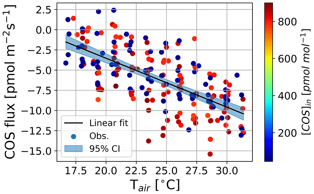
Figure 1. Measurements of COS flux at different air temperatures in the empty chamber.
Dots represent measurement data points and their colors indicate injected COS mole fractions in a chamber, black lines are linear fit equations, and filled areas indicate 95 % confidential interval.
2.1.2. Experiments. Table 1 lists the environmental factors that were used in the three experiments. We manipulated inflowing COS mole fractions, humidity, and air temperatures while keeping other environmental conditions constant, as specified in each experimental design. All environmental changes were introduced gradually to allow the leaf sufficient time to adapt to chamber conditions. For instance, we applied humidity (to achieve a desired gsw) and temperature changes of approximately 0.8 mol m−2 s−1 and 10 °C, respectively, over a period of two hours. This gradual adjustment ensured that measurements reflect steady-state conditions and minimize transient effects from rapid environmental changes. To exclude the effects of light on VCOS and VCO2, we maintained a high light intensity, similar to growth conditions, of 600 µmol m−2 s−1 throughout the experiments.
Table 1. Environmental conditions during the three experiments.
The range of controlled and constant variables for each experiment is expressed as minimum ~ maximum and mean ± standard deviation, respectively. Experiment 1 (Sunflower 1) aims to detect COS compensation points at two temperatures. Experiments 2 (Sunflower 2, 3, and 4) and 3 (Sunflower 2 and 4) are designed to investigate responses of VCOS and VCO2 to gs and gm, respectively. We controlled a designated variable in each experiment while other variables including light intensity, air flow rate, and mixing fan speed were kept constant.
Experiment
(Control) | Experiment 1 ([COS]in) | Experiment 2 (gsw) | Experiment 3 (Tleaf) |
|---|
Sunflower
number (-) | 1 | 1 | 2 | 3 | 4 | 2 | 3 |
gsw (mol
m−2s−1) | 0.8 ± 0.0 | 0.9 ±0.1 | 0.4 ~ 1.1 | 0.3 ~ 1.0 | 0.3 ~ 0.6 | 0.6 ± 0.1 | 0.6 ± 0.0 |
| VPD (kPa) | 0.5 ± 0.0 | 0.5 ± 0.0 | 0.6 ± 0.1 | 0.7 ± 0.2 | 0.9 ± 0.3 | 0.7 ± 0.2 | 0.9 ± 0.3 |
| Tleaf (°C) | 19.8 ± 0.0 | 25.0 ±0.3 | 25.1 ± 0.0 | 26.4 ± 0.1 | 24.8 ± 0.3 | 19.1 ~ 30.9 | 19.0 ~ 29.8 |
[COS]in
(pmol m−2s−1) | 94.11 ~ 589.05 | 104.50 ~ 706.96 | 1096.4 ± 12.6 | 1181.9 ±
11.1 | 914.4 ± 29.6 | 1087.7 ±
41.1 | 926.8 ±
14.0 |
[CO2]in (µmol
m−2s−1) | 446.5 ± 0.1 | 449.1 ± 0.3 | 441.0 ± 0.4 | 446.2 ±
1.5 | 447.5 ± 1.7 | 439.9 ± 3.1 | 447.3 ± 1.4 |
The first experiment (Experiment 1) aimed to detect COS compensation points and their temperature dependence. To determine the existence of ΓCOS and its temperature response, we measured FCOS at four distinct inflow COS mole fractions ranging from 94 to 589 pmol mol−1 at two different leaf temperatures (19.8 °C and 25.0 °C). As in Gimeno et al. (2017), the values of the ΓCOS were subsequently calculated for each temperature by extrapolating the COS mole fraction at which FCOS reaches zero using a linear regression.
The second experiment (Experiment 2) aimed to compare responses of COS and CO2 uptake to stomatal closure. We examined the responses of VCOS and VCO2 to gsw while keeping other environmental factors constant, including air temperature (approximately 25 °C). Thus, changes in VCOS and VCO2 predominantly reflect responses to changes in gsw. The modulation of gsw was accomplished by adjusting humidity within the leaf cuvette – hence modifying VPD – using the humidifier.
The last experiment (Experiment 3) aimed to compare responses of COS and CO2 uptake to changing temperatures. We observed VCOS and VCO2 while controlling the air temperature (Tair) within the leaf cuvette and maintaining other variables constant, including gsw. The desired gsw value was sustained by manipulating chamber humidity and thus VPD when necessary. The resulting leaf temperatures varied between 19.0 and 30.9 °C.
Regarding a repetition of experiments, Experiment 1 was executed once with a single sunflower plant (Sunflower 1), while Experiments 2 and 3 were replicated with three different sunflower plants over three days (Sunflower 2, 3, and 4). During the measurement of COS, CO2, and H2O mole fractions in Experiment 3, the complete temperature range could not be covered consistently across all three repetitions due to fluctuating gsw conditions. Due to this limitation, data from Sunflower 3 were omitted from the analysis of Experiment 3. Overall, we collected 15 data points from Experiment 1 and 48 data points from Experiments 2 and 3.
The measured VCOS and VCO2 were used to calculate the LRU (-), which was used to characterize differing response of COS and CO2 from Experiments 2 and 3:
where ACOS (pmol m−2 s−1) and ACO2 (µmol m−2 s−1) are assimilation rates of COS and CO2, respectively. These rates were normalized by outflowing concentrations [COS]out and [CO2]out.
2.2. Conductance model
2.2.1. General concept. Since the observations were somewhat limited in exploring internal leaf processes, we developed a conductance model and applied an optimization method using 48 data points from Experiments 2 and 3. Experiment 1 (15 data points) was used to provide initial information of ΓCOS and its temperature dependence to the model (Section 3.2.2).
Our leaf conductance model simulates the concurrent exchange of COS, CO2, and H2O in a plant leaf with the conditions of the laboratory experiments. Since these gases share the same stomatal pathway, their simultaneous modeling helps us understand the mechanisms of leaf conductance. The model assumes that gas exchange reaches equilibrium, a steady-state condition we tried to attain in the conducted experiments (see Section 2.1.1). All constant variables used in the model are listed in Table 2. Variables excluded from Table 2 are targets for optimization as explained in Section 2.3.
Table 2. Model constants used in the model.
Variables in all gases were used for all models, while those specific to COS, CO2, and H2O were applied to their respective model. The molar volume (Vm) is at standard temperature (298 K) and pressure (100 kPa).
| Gas | Symbol | Description | Unit | Value | Q10 |
|---|
| All | S | Leaf area | cm2 | 9.0 | |
| R | Universal molar gas constant | J K−1 mol−1 | 8.314 | |
| Vm | Molar volume | m3 mol−1 | 0.0248 | |
| Vcν | Cuvette volume | cm3 | 109a | |
| COS | ∆Ha,CA | Activation energy of CA | kJ mol−1 | 40b | |
| ∆Heq,CA | Enthalpy change of CA | kJ mol−1 | 100b | |
| CO2 | τ298K | Specificity factor between CO2
and O2 at 298 K | - | 2600c | 0.57 |
| Kc,298K | Michaelis-Menten constant for
carboxylation at 298 K | Pa | 30c | 2.1 |
| Ko,298K | Michaelis-Menten constant for
oxygenation at 298 K | Pa | 30000c | 1.2 |
| Rd | Dark respiration at 298 K | µmol m−2 s−1 | 3.0c | 2.0 |
| p[O2]i | Partial pressure of internal O2 | Pa | 20900c | |
| H2O | gmw | Mesophyll conductance for H2O | mol m−2 s−1 | 10 | |
Figure 2a illustrates the methodology for the gas exchange experiments. As described in Section 2.1.2, environmental conditions, including [COS]in, Tair, and VPD, were manipulated to test the hypotheses while keeping other variables, such as light levels, constant. The cuvette received controlled mole fractions of the three gases via the airflow. Figure 2b depicts the exchange pathways of COS, CO2, and H2O within the sunflower leaf, which form the basis for the conductance model. We assumed that COS, CO2, and H2O production or consumption within the plant were governed by three conductances: boundary layer conductance (gb (mol m−2 s−1)), stomatal conductance (gs (mol m−2 s−1)), and mesophyll conductance (gm (mol m−2 s−1)) limited by physical or biochemical processes
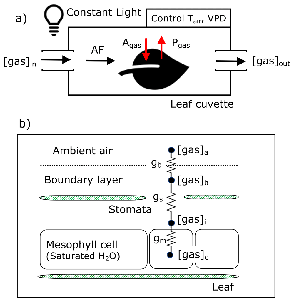
Figure 2. Schemes of leaf cuvette experiments (a) and diffusion pathways of COS, CO2, and H2O into and out of a leaf in the conductance model (b).
Agas and Pgas indicate the assimilation rate and production rate of each gas. gb, gs, and gm represent boundary, stomatal, and mesophyll conductance, respectively.
With a designated set of conductance values, the model simulates the mole fractions of the three gases in each layer: ambient air ([gas]a), boundary layer ([gas]b), and inter-cellular airspace ([gas]i)), and mesophyll level ([gas]c). The mole fractions of COS, CO2, and H2O are represented in units of pmol mol−1, µmol mol−1, and mmol mol−1, respectively.
The following rate equations describe the gas exchanges tendencies, assuming they achieve a steady state:
Here, Vm (m3 mol−1) is the molar volume, and Vcv (m3) is the cuvette volume. To account for the different properties of COS and CO2 to H2O, the stomatal conductances (gs,COS and gs,CO2) and the boundary layer conductances (gb,COS and gb,CO2) are scaled proportionally to the conductance of water vapor (gsw and gbw) (gs,CO2 = gsw/1.6, gb,CO2 = gbw/1.4, gs,COS= gsw/1.94, gb,COS = gbw/1.56) (Bonan, 2008; Seibt et al., 2010; Stimler et al., 2010).
For the COS and CO2 exchange at the stomatal level, a ternary system with H2O and air should be considered, because the transpiration (FH2O (mol m−2 s−1)) is significantly larger than COS and CO2 assimilation (Jarman, 1974; von Caemmerer & Farquhar, 1981). Thus, we added the ternary term in Equation 4 and Equation 5 for the COS and CO2 models:
Considering the H2O ternary system is important, but it did not significantly impact the calculations of mole fractions. To investigate the effects of [gas]i to flux to evaluate Hypothesis 2, we calculated flux using Equation 3, Equation 6, Equation 7:
Here, gb∼s denotes the conductance from the leaf boundary layer to the stomata. The deposition velocity (Vgas (mol m−2 s−1)) can be calculated as follows:
Here, (1-[gas]i [gas]a-1) represents the effect of changes between internal and ambient mole fractions on the gas conductance and deposition velocity, and this term is named Ambient Fraction Remaining (AFR). This concept is utilized in Section 3.2.3 for interpreting Hypothesis 2.
This set of coupled rate equations can be solved analytically, resulting in mole fractions of the three gases in each layer. Conductance at the mesophyll level (gm) and [gas]c were calculated using a different model for each gas. Descriptions of the individual biophysical processes at the mesophyll level for each gas are provided in subsequent sections.
From experiments, we measured [gas]out, while the leaf conductance model calculates [gas]a. To interpret experimental results using the leaf conductance model, [gas]out,est was used for [gas]a because thorough mixing ensures they are the same. In the model, the estimated mole fractions for COS and CO2 are based on wet air. As [gas]out,obs of COS and CO2 are based on dry air, we eliminated the diluting effects of H2O from [gas]out,est and the equivalent dry mole fraction is:
where [H2O]out,obs is the observed outgoing H2O mole fraction (mmol mol−1).
Since [COS]in,obs was measured after moisture removal, we used Equation 10 to convert [COS]in,obs from a dry air basis to wet air basis for use in the conductance model, substituting [H2O]in,obs for [H2O]out,obs.
Finally, net fluxes of the three gases were calculated using the same methodology as employed for the observations (Equation 1).
2.2.2. Water vapor model. In our experiments, we observed water evaporation from leaves. We aimed to model this evaporation at the mesophyll level and its subsequent transport out of the leaves, governed by gsw. The unit of H2O mole fractions in all layers is mmol mol−1, and the unit of the flux is mmol m−2 s−1.
[H2O]c was calculated assuming that water vapor within the mesophyll intercellular airspace is saturated. However, we allowed for relative humidity within the intercellular airspace (RHi (%)) to be less than 100 %, based on previous studies (Cernusak et al., 2018; Wong et al., 2022). To achieve this, we introduced a mesophyll conductance for water vapor (gmw) and set it to an arbitrary value of 10 mol m−2 s−1, approximately ten times the largest observed value of gsw.
We introduced a mesophyll conductance for water vapor (gmw) of 10 mol m−2 s−1. The expression for [H2O]c relies on Tleaf (°C) and air pressure (Pair (Pa)):
Using these assumptions, we calculated the water vapor mole fractions in the atmosphere ([H2O]a), boundary layer ([H2O]b), and interior ([H2O]i) by solving Equation 3, Equation 4, and Equation 5. Finally, we estimated the RHi (%) from the calculated [H2O]c and [H2O]i :
2.2.3. CO2 model. We aimed to simulate the gross CO2 flux (FCO2, µmol m−2 s−1) and mole fractions of CO2 in each layer (µmol mol−1) using the model proposed by Farquhar et al. (1980). In this model, the gross CO2 uptake rate is calculated as the minimum value among assimilation limited by enzymes (Am), light (AE), and sucrose synthesis (AS), minus the dark respiration (Rd) :
Our experiments were conducted under a constant light intensity (PAR = 600 µmol m−2 s−1). We assumed that the AE and AS pathways were saturated, as light saturation points previously were obtained above 500 µmol m−2 s−1 (Lobo et al., 2013). Consequently, we calculated gm,CO2 ([CO2]i − [CO2]c) in Equation 7 with Am −Rd. Rd was estimated by Collatz et al. (1991).
Am is calculated by multiplying the maximum rate of RuBisCO carboxylation (Vmax,Rub) with the partial pressure changes from RuBP partitioning between the CO2 carboxylation and O2 oxygenation reactions:
where p[CO2]i (Pa) and p[O2]i (Pa) are the partial pressures of CO2 and O2 in the inter-cellular air space. Kc (Pa) and Ko (Pa) are Michaelis-Menten constants for CO2 and O2, respectively. Γ∗CO2 (Pa) stands for the CO2 compensation point independent of dark respiration. The estimation of Γ∗CO2 is based on the partial pressure of oxygen linked to the side reaction of RuBisCO:
Here, T2 corresponds to Tleaf, and T1 is 25 °C for the CO2 parameters Kc, Ko, and Γ∗CO2. The temperature function of Vmax,Rub (µmol m−2 s−1) at Tleaf (°C) is calculated by (Badger & Collatz, 1977):
where ∆Ha,Rub (J mol−1) is the activation energy of RuBisCO, valued at 60.0 kJ mol−1 (von Caemmerer & Evans, 2015), and Tref,Rub (K) is the reference temperature (298 K). R is the universal molar gas constant (8.314 J K−1 mol−1).
2.2.4. COS model. We constructed the COS model to estimate the gross COS flux rate (FCOS, pmol m−2 s−1) and mole fractions of COS in each layer (pmol mol−1).
The biochemical conductance of COS in the mesophyll (gm,COS (mol m−2 s−1)) was calculated using the temperature function of CA, based on an specified Arrhenius equation and Michaelis-Menten Kinetics (Cho et al., 2023; Daniel et al., 2010; Ogée et al., 2016; Sun et al., 2015):
Here, Vmax,CA (mol m−2 s−1) is the maximum catalyzation velocity of CA, ∆Ha,CA (J mol−1) represents the activation free energy of CA and ∆Heq,CA (J mol−1) is the enthalpy change when the enzyme transits from activation to inactivation. Teq,CA (°C) stands for the optimum temperature at which the concentrations of activated and inactivated enzymes are equal (Daniel et al., 2010; Ogée et al., 2016; Sun et al., 2015). We adopted the normalization factor AT as the value of fCA(Teq,CA)−1.
Lastly, we applied the ΓCOS into [COS]c. We proposed four temperature functions of ΓCOS based on Experiment 1 data. For model S1, ΓCOS was set to zero across all temperatures, assuming no compensation point effects. For model S2, ΓCOS was represented as a linear function:
where Tref (°C) is the intercept temperature (16.4 °C), determined from the linear regression of two ΓCOS values detected in Experiment 1 (Section 3.1.1). The slope mCOS (pmol mol−1 K−1) was set to 16.2 pmol mol−1 K−1, also derived from Experiment 1. At low temperatures, where ΓCOS becomes negative, we assumed ΓCOS = 0.
For model S3, ΓCOS was calculated using the Arrhenius function with a observation-based value of 55.0 pmol mol−1 at 293 K from Experiment 1:
and for model S4, ΓCOS was similarly computed using a reference value of 138.7 pmol mol−1 at 298 K:
where ∆Ha,Γ (kJ mol−1) represents the activation energy for ΓCOS. By solving for ∆Ha,Γ using the two derived ΓCOS values, we determined an initial activation energy of 134.3 kJ mol−1.
These four ΓCOS functions (S1–S4), along with their imposed uncertainties, are visualized in Figure 3.
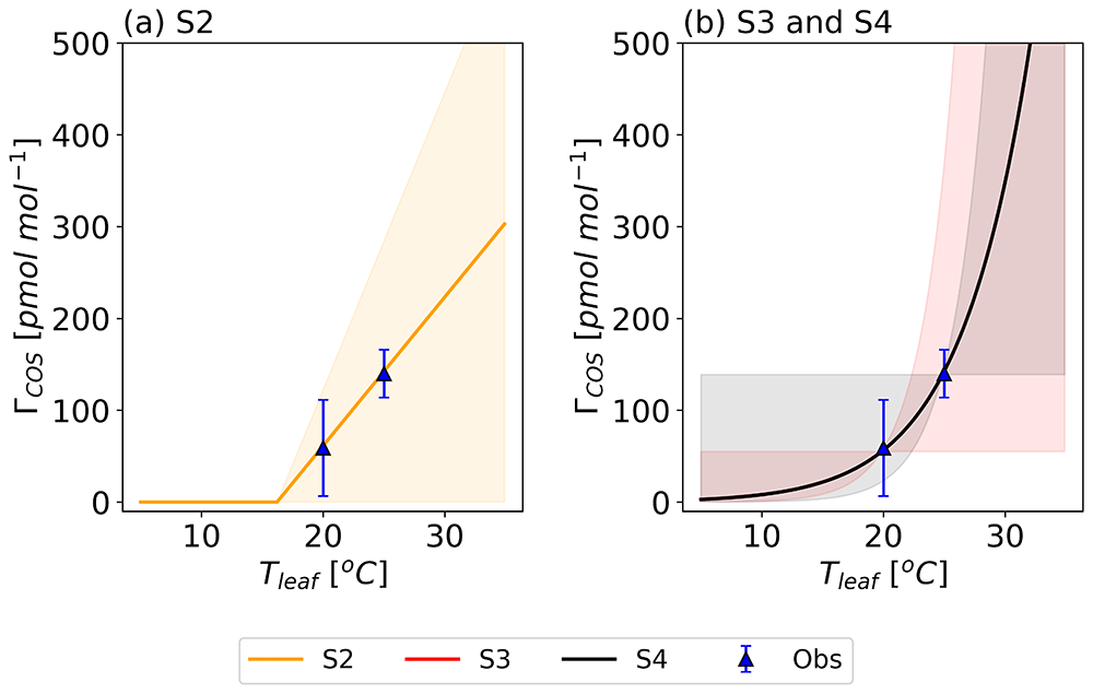
Figure 3. Prior temperature functions of the COS compensation point (ΓCOS) (lines) with their error ranges (shaded area) compared to the regression-derived ΓCOS from Experiment 1 (blue triangles and error bars corresponding dataset in Figure 4).
The S1 model assumed ΓCOS = 0 pmol mol−1. Model S2 describes ΓCOS as a linear relationship with Tleaf (a), while models S3 and S4 use an Arrhenius equation (b).
2.3. Indirectly derived COS compensation point
To support the robustness and consistency of our analysis to detect ΓCOS, we incorporated the indirectly derived ΓCOS from 48 data points in Experiments 2 and 3. We calculated [COS]c, equivalent to ΓCOS, using our optimized model parameters in Equation 3, Equation 6, and Equation 7. First, we calculated [COS]b from the measured COS mole fractions with the rearranged Equation 3:
where [COS]in and [COS]a, along with AF, S, and gb,COS, were applied from Experiments 2 and 3. Due to thorough mixing within the cuvette, we assumed [COS]out to be equivalent to [COS]a and used it accordingly (refer to Section 2.2). Here, [COS]in and [COS]out were converted a dry air basis to a wet air basis. We then used the derived [COS]b to calculate [COS]i using the rearranged Equation 6:
FH2O was calculated using Equation 1 with the observed [H2O]in and obtained [H2O]a by the H2O model. We used optimized gsw value in the H2O model and gs,COS. The reason for using the model-calculated [H2O]a instead of the observed [H2O]out is to consider the optimized gsw in FH2O.
[COS]i is then used in Equation 7 to derive [COS]c :
where gm,COS was determined using Equation 18 with optimized parameters Vmax,CA and Teq,CA.
It is important to note that these indirectly calculated ΓCOS values vary depending on the chosen temperature-dependent functions of ΓCOS, which influence other parameters. Note that indirect derived ΓCOS values differ from ΓCOS functions due to their impact on the optimized parameters used in the calculations.
2.4. Parameter optimization
2.4.1. Optimization setting. Beginning with the model state parameter (x), we calculated [gas]out,est and compared these to the observed values [gas]out,obs. We aimed to minimize the differences between our model and the observations during each optimization step. To accomplish this, we defined a cost function (Jtot) consisting of a background term (Jbg) and three observational terms that account for the differences between model estimations and observations of COS (JCOS), CO2 (JCO2), and H2O (JH2O):
The first term of the cost function penalizes deviations of the state x from the prior state vector xa. This penalty depends on σ, which represents the prior error in the state vector. This background term is introduced to keep state variables within reasonable boundaries (Brasseur & Jacob, 2017). The last three terms of the cost function calculate the costs associated with deviations between modeled ([gas]out,est) and observed mole fractions ([gas]out,obs) for COS, CO2, and H2O. Each term is balanced by optimization weights (Wbg, WCOS, WCO2, and WH2O) to account for the differences in background and observational errors. The detailed determination of these weights is provided in the following section.
The costs related to observations (JCOS, JCO2, and JH2O) are influenced by observational errors (σCOS, σCO2, and σH2O), derived from the measured COS, CO2, and H2O mole fractions. These observational errors were determined as the standard deviation of the measured mole fractions at outflow within the the data point interval (150-second). Formally, σCOS, σCO2, and σH2O should also reflect model errors caused by model parameters not included in the state or by processes that were not modeled (Brasseur & Jacob, 2017). Note that we excluded data from Experiment 1 to validate the optimized temperature function of ΓCOS in Section 3.2.2.
Due to the larger relative error in [H2O]out,obs and [COS]out,obs than in [CO2]out,obs, the optimization procedure tended to focus on minimizing preliminary JCO2. To better utilize the non-CO2 observations, we introduced optimization weights for each cost component. The observed [CO2]out,obs values ranged from 379.4 to 390.0 µmol mol−1, with an average observational error of only 0.2 µmol mol−1 (0.05 %). [COS]out,obs values ranged from 748.2 to 1032.4 pmol mol−1, with an average error of 16.7 pmol mol−1 (1.91 %). [H2O]out,obs values ranged from 15.2 to 32.5 mmol mol−1 with a mean error of 0.3 mmol mol−1 (1.14 %).
The targeted state parameters, along with their initial values and errors, are listed in Table 3. We assumed that the parameters related to the temperature response of mesophyll cells are consistent across all experiments, as all sunflowers were cultivated in a similar climate. We constructed state vectors with variables that significantly impact the total cost and better quantify the combined leaf exchanges: Vmax,CA, Teq,CA, and mCOS for COS, Vmax,Rub and ∆Ha,Rub for CO2, and gsw for all gases.
Table 3. State parameters (x) and their prior and posterior values with their errors based on model S2.
Posterior errors are calculated from 200 optimizations in a Monte Carlo method (Section 2.5). The last column denotes the error reduction. Prior and Posterior values for gsw are averaged values across the dataset from Experiments 2 and 3. Values in "Bounds" column with brackets indicate lower and higher bounds provided to the optimization.
| Parameter | Description | Unit | Bounds | Prior ± Error | Posterior ±
Error | (b-a)/a1
(%) |
|---|
| Vmax,CA | Maximum velocity
for CA | mol m−2 s−1 | [0.01, 0.50] | 0.125 ± 0.060 | 0.217 ± 0.0372 | 38 |
| 0.189 ± 0.0293 | 52 |
| 0.230 ± 0.0424 | 30 |
| Teq,CA | Optimum
temperature for CA | °C | [1, 60] | 30.0 ± 15.0 | 39.7 ± 5.0 | 66 |
| mCOS | Slope of ΓCOS | pmol mol-1 K-1 | [1, 300] | 16.2 ± 16.2 | 22.4 ± 5.3 | 67 |
| Vmax,Rub | Maximum velocity
for RuBisCO | µmol m−2 s−1 | [1, 200] | 90.0 ± 20.0 | 94.4 ± 0.32 | 98 |
| 87.4 ± 0.53 | 98 |
| 82.9 ± 0.34 | 98 |
| ∆Ha,Rub | Activation energy for
RuBisCO | kJ mol-1 | [1, 100] | 60.0 ± 12.0 | 54.5 ± 0.9 | 92 |
| gsw | Stomatal
conductance of H2O | mol m−2 s−1 | [0, 3] | 0.62 ± 0.09 | 0.64 ± 0.05 | 43 |
Although we selected sunflower leaves at similar development stages, variations in biochemical functioning existed among individual leaves. Therefore, we optimized Vmax,CA and Vmax,Rub for each individual plant, as these largely determine mesophyll conductance (Cho et al., 2023; Le Roux et al., 2001; Williams & Flanagan, 1996). The initial Vmax,CA was based on the averaged Vmax,CA across different phenological stages from two observation sites, Hyytiälä (Finland) and Harvard Forest (United States), as introduced by Cho et al. (2023). The standard deviation of Vmax,CA was used as the state error. For Vmax,Rub, we set the initial value as Vmax,CA divided into the scaling factor 1400, derived from laboratory measurements of gas exchange in C3 plants (Berry et al., 2013; Stimler et al., 2010; Stimler et al., 2011).
Teq,CA is more crucial in determining CA’s temperature function compared to other kinetics variables (Cho et al., 2023). For Teq,CA, we used the initial value and state error reported by Cho et al. (2023).
To determine the temperature dependence of ΓCOS, we evaluated four different functions (S1 to S4) within the conductance model. Each function was optimized and compared against observation-based ΓCOS. The S1 model excludes ΓCOS, while S2 applies a linear function with mCOS of 16.2 pmol mol−1. Both S3 and S4 use a temperature dependence described by an Arrhenius relationship. All models were initialized with the same prior error for ΓCOS, including the zero-compensation point, as shown in Figure 3.
For the CO2 parameters, we optimized ∆Ha,Rub, as it is an unknown parameter for Sunflowers. We determine the initial value and error of ∆Ha,Rub using the mean and standard deviation across nine species reported by von Caemmerer and Evans (2015). Other temperature-dependent parameters were adopted from Collatz et al. (1991).
Although the Li-6800 is a well-developed and accurate gas exchange analysis system, we optimized gsw for each experiment to account for any potential observational errors resulting from several assumptions, such as the parameter K described in Section 2.1.1. Initial values for gsw were taken from the LI-6800 measurements during Experiments 2 and 3. We applied a random error of 0.08 mol m−2 s−1, representing the standard deviation of gsw from Experiment 3, despite efforts to maintain a constant gsw (± 0.06 mol m−2 s−1) and considered an extra measurement error (0.02 mol m−2 s−1). Additionally, we added individual [H2O]out,obs errors by normalizing [H2O]out,obs. The averaged initial gsw value and its standard deviation (prior error) are 0.61 mol m−2 s−1 and 0.09 mol m−2 s−1, respectively.
Assuming a Gaussian probability density function for the state parameters could lead to nonphysical values in the optimization process. Thus, we minimized Jtot using the Sequential Least SQuares Programming optimizer (SLSQP) from the SciPy Python library. This optimizer enables the specification of lower and upper bounds on the state space and is well-suited for solving nonlinear problems. The parameter bounds are listed in Table 3.
2.4.2. Weight determination. We selected weights to achieve more balanced prior costs across four components in Equation 25. The prior chi-squared value (χ2prior) was used to check the cost balance in prior condition. We set seven possible weights, and the corresponding χ2prior value ranged from 3 to 200, as listed in Table 4. Then, we optimized parameters and calculated cost reduction rates for each part of the cost function. For H2O, we found a χ2prior value of about 3, indicating that the H2O model already performs well with the prior parameter settings.
Table 4. Candidates for weights in the observational terms (WCOS, WCO2, WH2O) based on the chosen χ2prior values.
| χ2prior | WCOS | WCO2 | WH2O
|
|---|
| 3 | 0.337 | 238.8 | 3.24 |
| 10 | 0.101 | 71.6 | 0.97 |
| 30 | 0.034 | 23.9 | 0.32 |
| 50 | 0.020 | 14.3 | 0.19 |
| 100 | 0.010 | 7.2 | 0.10 |
| 150 | 0.007 | 4.8 | 0.06 |
| 200 | 0.005 | 3.6 | 0.05 |
We finally selected the weight combination that minimized the averaged reduction rates of JCOS and JCO2 and ensured that each χ2poste exceeded the value of 0.6 to avoid over-fitting, including Jbg. The selected weights (WCOS =0.034, WCO2 = 7.2, WH2O = 3.24, Wbg = 1.0), correspond to χ2prior values of 30, 100, and 3 for COS, CO2, and H2O, respectively. These weights lead to a more balanced ratio of χ2prior across the observational parts (COS : CO2 : H2O = 10 : 33 : 1), compared to the ratio without weights (1 : 329 : 4). Note that the prior value of Jbg is zero by design.
2.5. Error statistics
We evaluated the model performance using χ2 values, mean bias errors (MBEs), and root mean square errors (RMSEs). The χ2 metric was calculated by dividing the partial cost function by the number of observations or state variables (Tarantola, 2005). A posterior chi-squared value (χ2poste) of 1 indicates a good fit, as the model predictions fall within the error distribution fall within the error distribution of the observations. A χ2poste significantly greater than 1 indicates a poor fit, while a value smaller than 1 suggests potential overfitting. MBE indicates bias, with a positive value for overestimation and a negative value for underestimation. RMSE is the quadratic mean of the differences between estimation and observation, with a value of 0 indicating a perfect fit.
Note that the optimization process targets for χ2poste to reach 1.0, but we also give the improvement in MBEs and RMSEs for completeness. To assess the posterior error associated with the optimized state, we employed a Monte Carlo method. In this process, we optimized the parameters using 200 distinct ensemble members, introducing random noise within the bounds of the respective state and observational errors (Bosman & Krol, 2023; Chevallier et al., 2007; Cho et al., 2023).
Furthermore, we conducted 500 perturbed forward simulations to assess the spread in both prior and posterior models. Parameters were randomly sampled from Gaussian distributions of both the prior and posterior. Prior uncertainties were assumed uncorrelated, while for the posterior parameters, we used the correlations that were determined using the Monte Carlo optimization. We quantified the posterior covariance matrix and considered the cross-parameter correlations when sampling the parameters to evaluate the posterior model. Parameters more than three standard deviations from the mean were discarded. These simulations were conducted with designated environmental input variables: pressure = 103,100 Pa, air flow rate (AF) = 0.00035 mol s−1, [CO2]in = 400 µmol mol−1, [COS]in = 1000 pmol mol−1, [H2O]in = 15 mmol mol−1, gbw = 2.44 mol m−2 s−1, gsw = 0.6 mol m−2 s−1, and Tleaf = 25 °C. We only varied one variable at the time, to evaluate its impact on the simulation.
3. Results
3.1. Experiments
3.1.1. COS Compensation Point (Experiment 1). Figure 4 presents the results from Experiment 1 with Sunflower 1, aimed at determining ΓCOS by measuring FCOS while controlling [COS]out and maintaining constant gsw and Tleaf. Minor fluctuations in gsw occurred during temperature adjustments, resulting in an approximately 20 % increase at higher temperatures. FCOS shows a linear increase with increasing [COS]out, in agreement with findings from earlier studies (Gimeno et al., 2017; Kesselmeier & Merk, 1993; Stimler et al., 2010). We quantified the regression-based ΓCOS using a linear function at two temperatures: ΓCOS was 55.0 ± 53.2 pmol mol−1 at 19.8 °C and 138.7 ± 26.1 pmol mol−1 at 25.0 °C (error estimates denote 95 % confidence interval). These results indicate that ΓCOS increases with rising Tleaf, suggesting a potential temperature dependence.
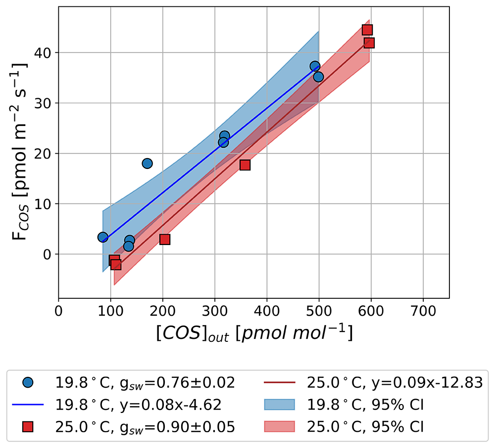
Figure 4. Observed mean COS net flux (FCOS) along an outflowing COS mole fraction ([COS]out) in the light at 25.0 °C (rectangle and red areas) and 19.8 °C (circle and blue areas) in Experiment 1.
Lines and shaded areas represent linear fits with 95 % confidence intervals. Positive values in FCOS (y axis) indicate COS uptake, and negative values indicate COS emissions.
3.1.2. Responses to Stomatal Conductance (Experiment 2). Figure 5 illustrates the observed VCOS, VCO2, and LRU as functions of optimized gsw for three sunflowers. The observed values show that both VCOS and VCO2 decrease with declining gsw, albeit at a slower rate at higher gsw values. Specifically, as gsw decreases from 1.0 mol m−2 s−1 to 0.4 mol m−2 s−1, VCOS declines by approximately 40 %, compared to a decline of about 10 % in VCO2. This difference persists even after accounting for the gsw ratio between COS and CO2 (1.21).
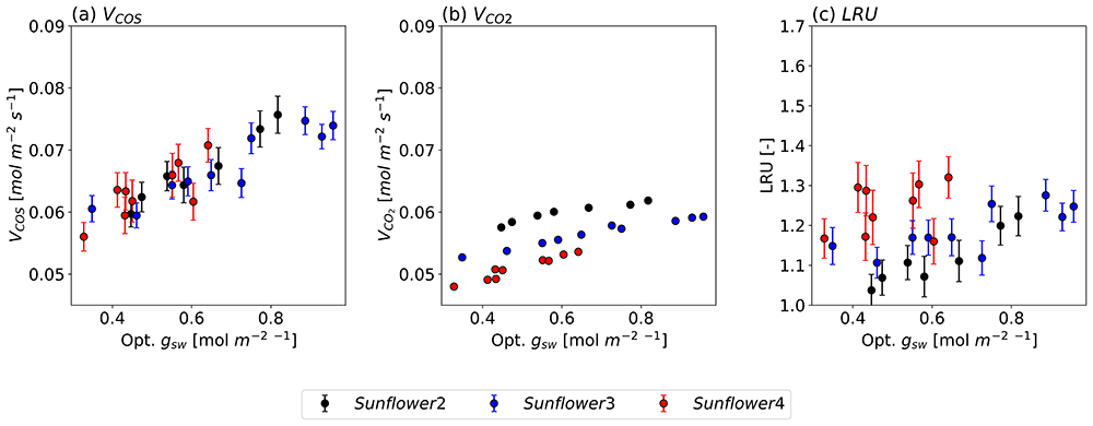
Figure 5. COS (a) and CO2 (b) deposition velocities and LRU changes (c) along the optimized gsw under leaf temperatures of approximately 25 °C for three different sunflower plants, each represented in a different color.
The circles and error bars represent the median values and standard deviations of the data points for their respective 150-second intervals.
The greater sensitivity of VCOS to changes in gsw is also reflected in the LRU, which consistently increases with gsw across all sunflowers. These findings support the hypothesis that COS uptake is more sensitive to variations in gsw compared to CO2 uptake. Meanwhile, slight differences in VCOS and VCO2 values among individual sunflowers result in variations in LRU as well.
3.1.3. Responses to Leaf Temperature (Experiment 3). Figure 6 shows the observed VCOS and VCO2, and LRU against Tleaf for two sunflowers, with gsw held approximately constant. For all sunflowers, VCOS decreases when temperatures exceed 25 °C, whereas VCO2 increases with Tleaf up to approximately 30 °C. The absolute rate of decrease in VCOS is larger than the rate of increase in VCO2. Consequently, LRU decreases as Tleaf increases. This trend can be attributed to the temperature responses of ΓCOS or/and the lower optimum temperature for CA than RuBisCO.
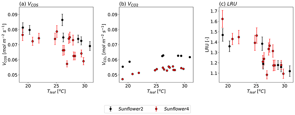
Figure 6. Same as Figure 5, but as a function of Tleaf with maintained stomatal conductance at 0.6 ± 0.1 mol m−2 s−1 (mean ± standard deviation).
The temperature-dependent variations in VCOS and VCO2 also differ slightly between individual sunflower plants. While VCOS exhibited relatively large observational errors, VCO2 showed minimal errors. This suggests that while experimental uncertainties may influence VCOS, the variations in both VCOS and VCO2 are likely driven by micro-environmental differences, plant-to-plant variability, or other natural conditions, even within the same species grown in similar environments.
3.2. Model-assisted analysis
3.2.1. Optimization Performance. We present the optimized results of model S2, as it provides the best fit to the observations (Section 3.2.2).
Table 5 quantifies how well the optimized model estimates [COS]out, [CO2]out, and [H2O]out compared to observations. The optimized model simulated the mole fractions of all three gases more accurately, reflected by mostly reduced values of χ2, MSE, and MBE. Notably, the model biases were mitigated, as shown by the low posterior MBE values for [COS]out (0.15 pmol mol−1), [CO2]out (– 0.01 µmol mol−1), and [H2O]out (0.07 mmol mol−1). The χ2poste values for [COS]out, [CO2]out, [H2O]out, and the state variables are 6.65, 1.68, 2.24, and 1.00, respectively. The large χ2poste and RMSE for [COS]out likely result from its relevantly larger observational error.
Table 5. The statistical indices of the prior and posterior estimated [COS]out, [CO2]out, and [H2O]out from model S2 compared to the observations with χ2 changes of state term (x).
The units of RMSE and MBE of [COS]out are pmol mol−1, [CO2]out is in µmol mol−1, and [H2O]out is mmol mol−1.
| Index | [COS]out | [CO2]out | [H2O]out | Background
(State x) |
|---|
| Prior | Posterior | Prior | Posterior | Prior | Posterior | Prior | Posterior |
|---|
| χ2 | 30.00 | 6.65 | 100.00 | 1.68 | 3.00 | 2.24 | 0.00 | 1.00 |
| RMSE | 16.71 | 7.93 | 3.63 | 0.71 | 0.30 | 0.45 | - | - |
| MBE | 11.77 | 0.15 | -1.52 | -0.01 | -0.14 | 0.07 | - | - |
Figure 7 presents scatter plots comparing the simulated atmospheric mole fractions from the prior and posterior models to the observed values. The optimized atmospheric mole fractions exhibit improved agreement with the observed values across all sunflowers, improving the performance of the prior simulations. The optimized model explains the variability in the observations with high R2 values from 0.93 to 0.99. The simulation errors, represented by the standard deviation of 500 forward simulations, were substantially reduced after optimization. Specifically for [COS]out, errors decreased from 47.4 pmol mol−1 to 12.5 pmol mol−1, for [CO2]out from 10.8 µmol mol−1 to 0.8 µmol mol−1, and for [H2O]out from 0.6 mmol mol−1 to 0.3 mmol mol−1. However, discrepancies remain, such as in Sunflower 2. Several posterior [COS]out and [CO2]out values of Sunflower 2 fall outside the weighted observational error range, likely due to measurement uncertainties.
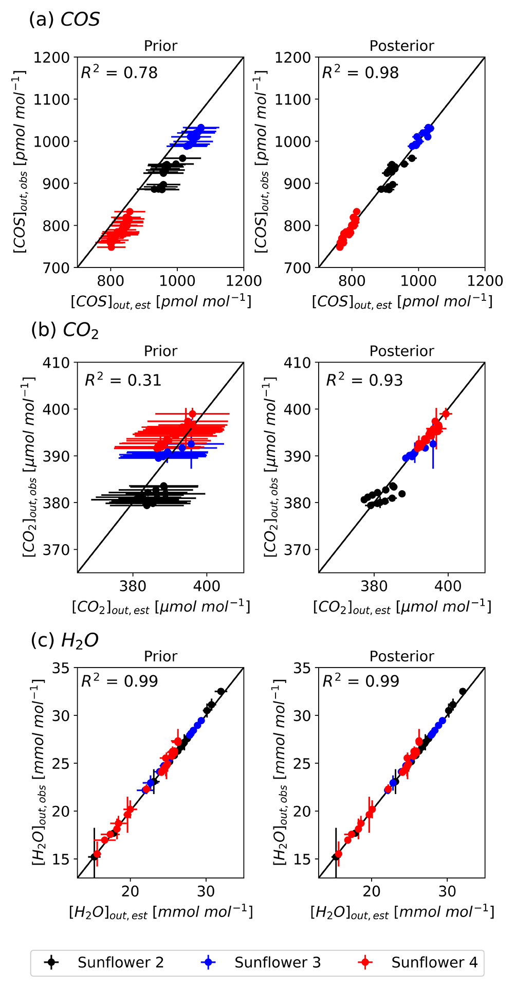
Figure 7. Scatter plots comparing the simulated (model S2) and observed atmospheric mole fractions of COS (a), CO2 (b), and H2O (c) with the prior parameters (left) and optimized parameters (right) with a 1:1 line indicating perfect agreement.
The vertical error bars represent weighted observational errors, taken as the standard deviations of measurements, and the horizontal error bars represent prior errors (left) and posterior errors (right). Colors indicate different sunflower plants (black: Sunflower 2, blue: Sunflower 3, red: Sunflower 4).
The optimized state values and their posterior errors, along with error reductions, are presented in Table 2. As expected, errors associated with all target parameters were significantly reduced, with an average error reduction of 48 %. An error reduction of more than 92 % was achieved for CO2 parameters ∆Ha,Rub and Vmax,Rub. Prior uncertainties of Teq,CA, mCOS, and Vmax,CA were reduced by more than 30 %, and the error reduction for gsw was about 43 %.
The optimized slope of ΓCOS (mCOS, 22.4 pmol mol−1 K−1) is slightly increased to the initial setting (16.2 pmol mol−1 K−1). With the optimized value of mCOS, the variable Teq,CA was adjusted to 39.7 °C, and the values of Vmax,CA for each plant were optimized ranging from 0.189 to 0.230 mol m−2 s−1. These values increased significantly from their priors, 30.0 °C and 0.125 mol m−2 s−1, indicating higher optimum temperatures and higher catalyzation velocities compared to the prior settings. The optimized Vmax,Rub ranged from 82.9 to 94.4 µmol m−2 s−1, while ∆Ha,Rub did not change substantially. The ratio of Vmax,CA to Vmax,Rub which is crucial for calculating CA activity from Vmax,Rub based on the assumption of a linear relationship, ranges from 2160 to 2770.
Comparisons of the optimized mean gsw values of 0.64 mol m−2 s−1 with the prior values of 0.62 mol m−2 s−1 reveal slight differences. Errors in gsw were reduced from 0.09 to 0.05 mol m−2 s−1. The optimized model yielded an average relative humidity within the leaf (RHi) of 98.82 ± 0.04 %.
Figure 8 illustrates the posterior covariance matrix derived from Monte Carlo calculations. Although several state variables were highly correlated after optimization (values above 0.7), they were retained as state parameters because their simulation errors were substantially reduced. For instance, three variables of COS parameters (Teq,CA, mCOS, and Vmax,CA) were highly correlated, with values ranging from 0.69 to 0.87, as these parameters are all related to the mesophyll uptake of COS.
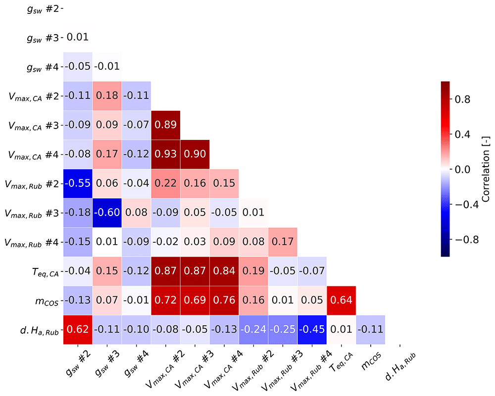
Figure 8. The covariance matrix for state variables.
Regarding gsw, only the first data point of each sunflower is marked.
3.2.2. COS Compensation Point (Hypothesis H1). Table 6 summarizes the changes in total cost (Jtot) between prior and posterior estimations for each ΓCOS temperature function. Among the tested models, the lowest total cost was achieved with the linear model (S2), followed by the Arrhenius models S4 and S3, and the model without a compensation point (S1). These results confirm that incorporating ΓCOS with a linear temperature function into the leaf exchange model provides the best agreement with observations, as it minimizes the overall cost function and improves model performance. However, the total cost difference between the S2 model and the S4 model was only 1 unit.
Table 6. Prior (Pri) and posterior (Poste) contributions to the cost function of the state term, H2O, CO2, and COS parts, depending on the prescription of ΓCOS and its temperature dependence.
Jtot is the sum of costs for the states (Jbg), H2O (JH2O), CO2 (JCO2), and COS (JCOS).
| No. | Description of ΓCOS | Cost |
|---|
| Jbg | JH2O | JCO2 | JCOS | Jtot |
|---|
| Function | Based T [°C] | Post | Pri | Post | Pri | Post | Pri | Post | Post |
|---|
| S1 | ΓCOS = 0 | - | 54 | 144 | 97 | 4800 | 80 | 2437 | 349 | 580 |
| S2 | Linear | 16.4 | 57 | 107 | 81 | 1440 | 320 | 564 |
| S3 | Arrhenius | 19.8 | 59 | 100 | 80 | 2634 | 335 | 574 |
| S4 | 25.0 | 61 | 106 | 80 | 2634 | 319 | 565 |
Figure 9 compares estimated ΓCOS with two types of observation-based values across temperatures. The first type is regression-based measurements from 15 data points at two temperatures in Experiment 1 (blue triangles; see Figure 4). The second type is indirect derived ΓCOS in Experiments 2 and 3.
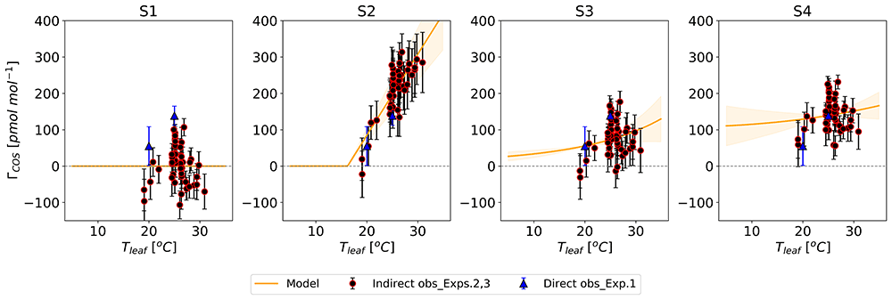
Figure 9. Posterior temperature functions for ΓCOS from S1 to S4 models, shown with orange lines and error ranges from 200 Monte Carlo simulations.
These are compared with ΓCOS values from Experiment 1 (blue triangles, regression-derived from two temperature points) and Experiments 2 and 3 (black circles with red edges, derived indirectly). Regression-derived ΓCOS measurements are 55.0 ± 53.2 pmol mol−1 at 19.8 °C and 138.7 ± 26.1 pmol mol−1 at 25.0 °C, detailed in Section 3.1.1). Indirectly derived values are averages with standard deviation error bars, calculated from parameters optimized through 200 Monte Carlo simulations (See Section 2.5.).
The optimized S2 model best captures the ΓCOS measurements derived from both regression and indirect methods, compared to other models. Specifically, the S2 model achieved the lowest RMSE with the indirect derived ΓCOS (39 pmol mol−1). The RMSE values for the other models were: S1 = 50 pmol mol−1, S3 = 49 pmol mol−1, and S4 = 41 pmol mol−1, respectively.
3.2.3. Response to stomatal conductance (Hypothesis H2). In Experiment 2, we confirmed that VCOS responds more strongly than VCO2 at low gsw values. To explore how changes in deposition velocity due to gsw are influenced by interactions with mesophyll conductance, we calculated AFR values (1 –[gas]i/[gas]a) for both gases using the optimized S2 model, as these values cannot be directly measured (Figure 10). Simulations were performed at a constant Tleaf of 25 °C.
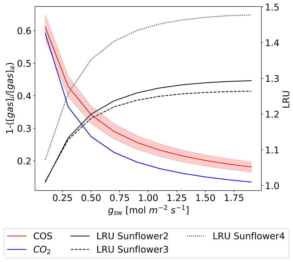
Figure 10. Simulated changes in (1 – [gas]i/[gas]a) for COS (red) and CO2 (blue) averaged among sunflowers 2, 3, and 4, with LRU (black, secondary y-axis) as a function of gsw each sunflower (Results from the S2 model).
The lines represent averages, and the filled areas indicate the standard deviation of 500 simulations using posterior error propagation.
The model results indicate that for both gases, AFR decreases as gsw increases, which provides support for Hypothesis 2. However, contrary to Hypothesis 2, which assumes that [COS]i is nearly zero thus resulting in AFR for COS close to 1, the actual modeled values range from 0.2 to 0.6 depending on gsw. This deviation indicates that [COS]i is not negligible and suggests a dynamic COS consumption within the leaf that does not bring [COS]i close to zero.
The model also reveals a distinct LRU pattern, showing sharp increases at low gsw values followed by stabilization at higher gsw. This response is consistent with observations from Experiment 2, where LRU exhibited similar trends in response to gsw. These results underscore the differing sensitivities of COS and CO2 uptake to gsw, as reflected in both experimental and modeled data.
3.2.4. Response to leaf temperature (Hypothesis H3). To investigate the temperature function of enzyme activity separated from ΓCOS in VCOS, we calculated gm,COS and gm,CO2 using the optimized model S2. Figure 11 shows the temperature dependency of gm,COS and gm,CO2 for three sunflowers. The magnitudes of these dependencies vary among plants due to differences in optimized Vmax values. The optimum temperature for gm,COS is around 35 to 40 °C, while for gm,CO2 it is approximately 35 °C, contrary to Hypothesis 3, which proposed a lower optimum temperature for gm,COS than gm,CO2.
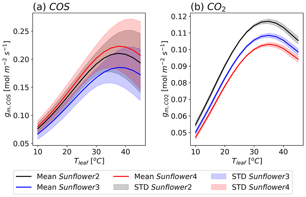
Figure 11. Modeled response of mesophyll conductances (gm) to leaf temperatures (Tleaf) for COS (a) and CO2 (b) with three sunflowers (black : sunflower 2, blue: sunflower 3, red: sunflower 4, results from the S2 model).
The lines represent averaged values, and the filled areas indicate the standard deviation from 500 simulations using posterior error propagation.
The observed decline in VCOS above 25 °C in Experiment 3 (Figure 6a) is explained by the model-predicted impact of ΓCOS on COS uptake. While the optimum temperature for gm,COS is approximately 35 to 40 °C, the influence of temperature-dependent ΓCOS results in a much lower optimum temperature for VCOS, around 20 °C. This is significantly lower than the optimum temperature for VCO2, which is approximately 30 °C.
The model results suggest that the temperature dependence of ΓCOS plays a critical role in shaping the distinct responses of VCOS and to temperature.
4. Discussion
4.1. Uncertainties in measurements and models
Through improvements in our experimental setup, especially with the LI-6800 system incorporating new gasket materials (Advanced Polymer, Polyethylene, and Neoprene) and optimized flow paths, we minimized the gas leakage issues prevalent in previous systems like the LI-6400. No significant pressure differentials were observed during experiments, supporting the effectiveness of these enhancements. Additionally, maintaining the cuvette under slight positive pressure reduces the risk of inward leakage.
Although leakage issues were minimized, the high uncertainty in COS measurements and models still requires careful interpretation. Model S2 was selected as the best model due to its minimal posterior costs and lowest RMSE with observation-based ΓCOS, despite higher H2O and background costs compared to S1, as shown in Table 6. Furthermore, the minor differences in posterior costs and RMSE with indirectly derived ΓCOS between S2 and S4 suggest that S4 is a viable alternative. The strong correlation between the temperature dependence of ΓCOS (mCOS) and Vmax,CA complicates the precise and independent determination of these two parameters. Accordingly, the exact value and temperature dependence of ΓCOS remain uncertain, but including a compensation point in the models, as in models S2 and S4, significantly improves their alignment with observations. Another point of consideration in our experiments is that our optimization was based on data from Experiments 2 and 3, conducted at temperatures ranging from 19.0 °C to 29.8 °C. Therefore, additional experiments across a broader temperature range are necessary to confirm the existence and assess the temperature dependence of ΓCOS.
In our experiment, we increased the COS mole fraction in the cuvette to approximately 1000 pmol mol−1, significantly above natural ambient levels, to enhance signal detection and reduce noise. The primary purpose of our empty chamber experiments was to eliminate the effects of emissions from chamber materials. Conducting these tests at similarly high mole fractions also helped mitigate any emissions that could arise from this higher mole fraction setting.
This high COS mole fraction possibly contributed to slightly higher AFR (Figure 10) because the high ambient mole fraction may influence the internal concentration. [COS]i/[COS]a values of about 0.63 ± 0.13 were observed under elevated ambient [COS]a conditions (Stimler et al., 2010), aligning with our results. Stimler et al. (2010) also reported a linear relationship between [COS]i/[COS]a and [COS]a, likely due to retro-diffusion from the leaves. Therefore, when applying our results to natural conditions ([COS]a about 500 pmol mol−1, the AFR may decrease. However, the high AFR is also possibly due to the influence of ΓCOS. The simulated [CO2]i/[CO2]a ranges from 0.4 to 0.9, consistent with values previously reported for C3 plants (0.5 – 0.8) (Black & Jones, 1985; Seibt et al., 2010; Tanner & Sinclair, 2015).
In Experiments 2 and 3, despite the high COS mole fractions, their consistent level throughout the experiments likely negated any impact on analyzing how gsw and temperatures relate to VCOS and VCO2.
In the model, only the enzyme CA is considered in determining the mesophyll conductance of COS. However, other enzymes, such as RuBisCO and phosphoenolpyruvate carboxylase (PEP-C), are known to catalyze COS uptake (Lorimer & Pierce, 1989; Protoschill-Krebs & Kesselmeier, 1992). The contribution of RuBisCO to COS uptake is relatively minor compared to CA (Protoschill-Krebs et al., 1996), and its activity has not yet been quantified.
4.2. Possible causes of a COS compensation point
COS emission can occur due to leaf stress induced by external factors during experiments. To minimize the risk of mechanical damage or stress, the chamber was gently attached, and leaves were inspected post-experiment for physical damage such as bruising, desiccation, or discoloration. No visible damage was observed, and the limited measurement duration further reduced the likelihood of stress-induced COS emissions.
Previous studies on COS leaf exchange experiments have reported positive ΓCOS values, but often concluded these are statistically indistinguishable from zero due to high variability. For example, Stimler et al. (2010) observed a ΓCOS of 60.7 pmol mol−1 at 25 °C, but due to experimental uncertainty, they considered it to be zero. Similarly, ΓCOS at 20.0 °C from our results was 55.0 ±53.2 pmol mol−1, making it also statistically insignificant. In contrast, our results show a significant ΓCOS at 25 °C (138.7 ±26.1 pmol mol−1). Previous studies, typically conducted below 25 °C, did not assess temperature dependence. Our modeling revealed a linear relationship between ΓCOS and temperature, consistent with Gimeno et al. (2017), who reported higher ΓCOS in mosses at elevated temperatures. Although no visible stress was observed in our plants, temperature stress may have influenced ΓCOS. Gimeno et al. (2017) suggested that COS emissions could result from protein degradation under stress, releasing COS through the breakdown of sulfur-containing amino acids. This highlights the role of temperature-driven biochemical pathways in shaping ΓCOS values and supports the inclusion of ΓCOS in leaf gas exchange models.
Differences in species physiology also contribute to ΓCOS. Mosses studied by Gimeno et al. (2017) exhibited higher ΓCOS values than in vascular plants, likely due to enzymatic activity of associated fungi and bacteria. While microbial activity is not directly applicable to vascular plants, it underscores the importance of species-specific factors in determining COS emissions. In vascular plants, rapeseed is known to produce COS due to its high sulfur content, with ΓCOS exceeding 100 pmol mol−1 during ripening and senescence (Belviso et al., 2022). However, no experiments have previously been conducted to detect ΓCOS in sunflowers.
Phenological stages also possibly influence COS emissions. Kesselmeier and Merk (1993) reported ΓCOS values ranging from 57 to 328 pmol mol−1 in rapeseed and corn during flowering, and Maseyk et al. (2014) found that COS uptake in wheat transitions from a sink to a source during ripening. In our study, measurements were conducted during the flowering phase, which could explain the observed COS emissions, although the exact source remains unclear. Sulfur emissions during senescence have been linked to the translocation of sulfur-containing amino acids and sulfur regulation in plant cells (Rennenberg, 1991).
Methodological advances may explain the discrepancies between our results and previous studies. We employed the Li-6800 system, which offers improved measurement accuracy, and evaluated an optimized conductance model incorporating temperature-dependent ΓCOS. Our findings confirm that all observations support an increase in ΓCOS with temperature.
The existence of ΓCOS and its increase at higher temperatures may result from a combination of the factors discussed above. Future research should explore the roles of plant phenology, microbial interactions, and environmental stressors to validate and extend these findings across various species and environmental conditions.
4.3. Impact of COS compensation point on Vmax,CA
The optimized ratio between Vmax,CA and Vmax,Rub ranges from 2160 to 2770, which is larger than previously obtained values of approximately 1200 from laboratory measurements with C3 plants (Berry et al., 2013). Kooijmans et al. (2021) reported an average ratio of 1616 ± 562 based on field observations in summer months. With our model that excluded ΓCOS (S1), we optimize a smaller Vmax,CA and thus obtain a smaller ratio, ranging from 1197 to 1327. Thus, models that incorporate ΓCOS result in higher optimized values of Vmax,CA and consequently to higher ratios between Vmax,CA and Vmax,Rub, indicating a higher maximum catalyzation velocity of CA.
4.4. Consequences for the COS global budget
Our evidence of decreasing VCOS between 20 and 25 °C (Figure 6a) supports lower biosphere uptake in high temperature regions. The current COS budget has a missing source of roughly 400 GgS year−1, mainly due to the large biosphere sink calculated by the Simple Biosphere model (SiB4) in the tropics (Berry et al., 2013). In warm tropical forests, biosphere uptake would be significantly reduced.
The presence of ΓCOS could have implications for the global COS budget and the utilization of COS in estimating GPP, especially under conditions such as drought, where high temperatures and low humidity persist. Despite the uncertainty concerning ΓCOS in our experiments, including ΓCOS in our model better reproduced CO2 and COS observations. This suggests that incorporating ΓCOS into global biosphere models could enhance the accuracy of COS flux estimates. Differences in temperatures and humidity responses between CO2 and COS should also be considered. To further improve the implementation of ΓCOS in biosphere models, it is recommended to measure ΓCOS and enzyme activity across diverse plant types, specifically tropical plants.
While our study focused on controlled conditions with a single species, larger variations would indeed be expected under natural conditions and across different species. Future research should therefore explore these factors in more diverse environmental settings to validate and generalize these findings.









