An understanding of the variety of life can be achieved by distinguishing between three key elements, as categorized by Heywood & Baste (1995): organismal (species) diversity, ecological (functional) diversity, and genetic diversity.
2.1. Capturing intra-species diversity (within and between individuals)
2.1.1. Use cases for chimerism
Currently, there is a lack of widely accepted standards for testing and evaluation of chimerism in multicellular organisms, including human chimeras (Rinkevich & Goulet, 2025). In cases of iatrogenic human chimerism (a frequent medical procedure), analysis typically involves identifying and quantifying specific genetic variations that distinguish donor cells from recipient cells, known as informative polymorphic markers. Monitoring changes in donor/recipient proportions over time (Rinkevich & Goulet, 2025) helps track the status of donor cell engraftment. Techniques for chimerism analysis include cytogenetics-based methods like fluorescent in situ hybridization (FISH) targeting sex chromosomes, as well as traditional molecular markers such as restriction fragment length polymorphism (RFLP), variable number of tandem repeats (VNTR), and short tandem repeat (STR) tests conducted via polymerase chain reaction (PCR), with reported sensitivities ranging from 1% to 5%. In recent years, more precise methods of chimerism analysis have emerged, capable of detecting variations down to fractions of a percent. These include real-time quantitative PCR (qPCR), digital droplet PCR (ddPCR), and next-generation sequencing (NGS) (Blouin et al., 2021; Blouin & Askar, 2022; Picard et al., 2023).
Natural chimerism is well documented in MAFs, primarily in soft corals (Barki et al., 2002; Giordano & Bramanti, 2021), hard corals (Frank et al., 1997; Jiang et al., 2015; Mizrahi et al., 2014; Puill-Stephan et al., 2009), colonial tunicates (Ben-Shlomo et al., 2001; Casso et al., 2019; Fidler et al., 2018; Paz & Rinkevich, 2002), and sponges (Blanquer & Úriz, 2011; Gauthier & Degnan, 2008; Maldonado, 1998; Mukai, 1992). In addition to morphological and histological observations utilized for tracking and identifying chimeric states in MAF species, multiple molecular techniques have been employed. These include random amplified polymorphic DNA-polymerase chain reaction (RAPD-PCR) analyses (Sommerfeldt et al., 2003) and amplified fragment length polymorphism (AFLP) profiles of chimerical combinations (Rinkevich & Yankelevich, 2004). However, microsatellite alleles have emerged as the most commonly utilized tool (Ben-Shlomo et al., 2001; Blanquer & Úriz, 2011; Guerrini et al., 2021; Pancer et al., 1995; Puill-Stephan et al., 2009; Rinkevich et al., 1998; Rinkevich et al., 2016; Schweinsberg et al., 2015; Stoner et al., 1999). A study investigating thresholds for microsatellite loci, involving 30 pairwise genotypic combinations and 330 chimeric mixtures, revealed that various genetic combinations may overlook chimerism, with the least common partner representing just 5–10% of the total DNA (Guerrini et al., 2021). More recent studies have combined the assessment of both IGH scenarios (microsatellites and somatic mutations) through the evaluation of single nucleotide polymorphisms (SNPs; see below).
2.1.2. Methodologies for establishing chimeras in corals and in colonial ascidians
Coral chimeras (both hard and soft corals) can only form during a brief window in early development; coral larvae may fuse at the planktonic stage, and young specimens can fuse up to 2–3 months post-settlement and metamorphosis (Barki et al., 2002; Frank et al., 1997; Shefy et al., 2021; Shefy et al., 2022). In contrast, chimeras in the botryllid ascidians can form between allogeneic adult conspecifics and throughout the organism’s lifespan (Rinkevich & Weissman, 1987b; Rinkevich, 2005).
Producing chimeras from the branching coral Stylophora pistillata (Figure 4)
1. Planula collection: Stylophora pistillata is a common Indo-Pacific branching species, commonly found from the very shallow waters down to 60 m depth (Shefy & Rinkevich, 2021). Collect planulae of S. pistillata nightly during the reproductive season, which lasts roughly 8–10 months per year (December/January to August/September) (Rinkevich & Loya, 1979; Shefy et al., 2018).
2. Trap setup: Use in situ planula traps to collect planulae (see Amar et al., 2007, for details). Select large colonies in shallow waters (15–25 cm diameter, 2–6 m depth). Each trap should consist of a floating plastic vessel connected to a 120-µm plankton net via a plastic funnel.
3. Trap placement: Place traps at sunset, and collect them after midnight or, more commonly, the following morning.
4. Transport to lab: Place collected traps in containers filled with fresh seawater and transport them to the lab.
5. Planulae counting: Rinse each net with filtered seawater (120 µm) to collect remaining planulae, then transfer them into Petri dishes. Rinse the traps’ containers with filtered seawater to release any attached larvae. Gravid colonies may release up to several hundred larvae per night.
6. Preconditioning dishes: Before collecting planulae, cover each Petri dish (bottom and sides) with a polyester film (“Maylor paper”; Jolybar, Israel) and precondition dishes for one month to develop microbial films that support coral larvae settlement (Shefy et al., 2021; Shefy et al., 2022).
7. Planulae placement: Place 20–40 planulae per dish. Submerge dishes to 75% of their height in a water table with running seawater to maintain ambient temperature, and cover with lids to reduce evaporation. Replace seawater daily to prevent mucus buildup and maintain natural salinity.
8. Daily monitoring: Monitor dishes daily, recording settlement rates, chimera formation, and survivorship. Note that planulae typically settle on the dish bottoms and walls.
9. Extended submersion: Most planulae will settle within the first week. Afterward, fully submerge the dishes in a water table with running seawater to allow spat establishment and additional chimera formation between closely situated spats (1–3 months).
10. Final attachment: Remove the Maylor paper from each dish, carefully cut between spats, and attach each chimera or individual, including the Maylor paper, to the chosen substrate using a drop of cyanoacrylate super glue. Alternatively, you can bend the Maylor paper to detach spats and glue them directly to substrates.
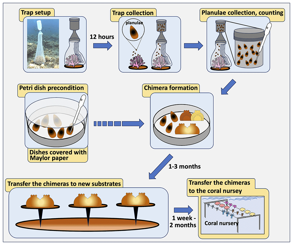
Figure 4. A flowchart for chimera formation in the branching coral Stylophora pistillata.
Producing chimeras from the colonial botryllid ascidian Botryllus schlosseri (Figure 5)
1. Animal description: B. schlosseri is a common, encrusting colonial sea squirt, likely originating from the Mediterranean, now spreading widely (Reem et al., 2022). It is also known as a model colonial species in basic and applied studies (Ben-Hamo & Rinkevich, 2021). Colonies inhabit shallow waters, attaching to rocks, algae, pilings, floats, and other substrates. Each colony consists of a few to thousands of genetically identical zooids (2–3 mm long), embedded within a gelatinous tunic. The zooids are arranged in star-shaped systems and connected through a blood vessel network with pear-shaped vascular termini (ampullae) extending to the colony's edges. For laboratory studies animals that are born and raised from oozooids under controlled conditions are preferable to animals directly collected from the field (Ben-Hamo & Rinkevich, 2021).
2. Colony maintenance: Keep each colony on 5 x 7.5 cm glass slides within glass staining racks in a 17-L glass tank (up to 20 colonies per tank). Replace seawater three times a week, maintain a 12:12 light cycle, and feed the colonies daily with commercial food or as previously described (Rinkevich & Shapira, 1998). Aerate each tank with an air stone, keeping water temperature at 20°C. Clean colonies weekly using a soft brush to remove debris and fouling organisms.
3. Chimerism potential: When two colonies come into contact naturally or in the lab, they either fuse their ampullae to form a vascular connection or develop cytotoxic lesions at the contact point (Magor et al., 1999; Rinkevich & Weissman, 1987c; Rinkevich, 2004b). This allorecognition system is genetically controlled by a single haplotype with codominantly expressed alleles, resulting in high polymorphism (Magor et al., 1999; Rinkevich, 2004b). Colonies can fuse with others, sharing at least one fusibility allele; rejecting colonies do not share fusibility alleles. Fusions are established 48–72 hours after the initial ampullae contact (Rinkevich & Shapira, 1999).
4. Isolating subclones: Following Rinkevich (1995), use a razor blade (it is best to use industrial blades) and brush to carefully clean the substrate around the colonies. Select small or large groups of zooids (1–4 systems) at the colony edges, ensuring that peripheral ampullae are long and extend outside the tunic. Cut between systems with a razor blade, isolate the growing edges without damaging the ampullae, and remove the subclones from the substrate.
5. Pairing subclones: Add a drop of water on a new, clean glass slide and then place subclones from two colonies, positioning them with a 1 mm gap between their ampullae. Absorb excess water. If ampullae are not well extended or were damaged during isolation, use cotton threads to secure the subclones to the substrate. For both, tied and untied subclones, place the slides in a moisture chamber (can be made of plastic or glass boxes) for 20–35 minutes to allow natural attachment to the substrate. Keep slides in the moisture chamber in a vertical position to remove excess water, allowing the ampullae to quickly attach to the substrate.
6. Chimera formation: Transfer slides with attached subclone pairs to 17-L standing seawater tanks for 24 hours, then move them to the seawater system. Hold slides vertically in glass staining racks, with up to five racks per tank. Observe daily, being cautious when removing slides from the tanks (in the first week), as subclones may detach easily.
7. Observations: Monitor daily for the first 1–2 weeks, then weekly. Document the number of buds and zooids, as well as signs of retreat growth (Rinkevich & Weissman, 1988) or colonial absorption (Rinkevich & Weissman, 1987b; Rinkevich et al., 1994).
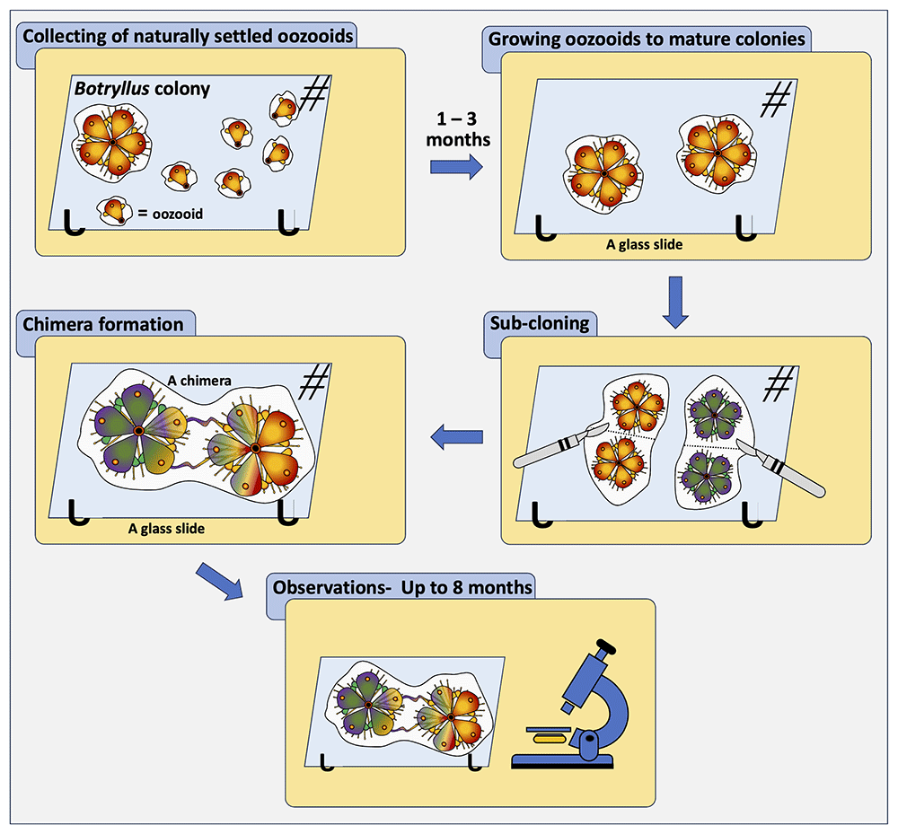
Figure 5. A flowchart for chimera formation in botryllid ascidians, worldwide-distributed colonial ascidian species of two genera, Botryllus and Botrylloides.
2.1.3 Use cases for somatic mutations
Somatic mutations are widespread among all multicellular organisms (Lynch, 2010). Due to the absence of germline and somatic cell segregation in many MAFs (Buss, 1983), germ cell differentiation occurs continuously from somatic stem cells in these taxa. Consequently, there is an increased likelihood of somatic mutations being integrated into the germ line, which are then passed on to larvae, maturing into juvenile corals. This process further facilitates a platform for selection and adaptation (Vasquez Kuntz et al., 2022). Over time, these somatic mutations progressively transform the genetically uniform MAF into a mosaic organism with distinct cell lineages (genetic mosaicism), where different regions of a single MAF organism exhibit divergent genetic compositions.
The identification of somatic mutations and mosaicism in MAFs is clarified through the application of microsatellites (Dubé et al., 2017; Maier et al., 2012; Olsen et al., 2019; Oury et al., 2020; Schweinsberg et al., 2014; Warner et al., 2016). More recently, mosaicism in MAFs is increasingly studied using SNP analysis (Casso et al., 2019; Chang et al., 2018; López-Nandam et al., 2023; Schweinsberg et al., 2015; Takata et al., 2021; Vasquez Kuntz et al., 2022). In some studies, the results are further validated through the utilization of RFLP and/or microsatellite alleles (Vasquez Kuntz et al., 2022), or by comparing Sanger electropherogram data with Illumina outcomes (López & Palumbi, 2020). Moreover, somatic mutations are differentiated from chimerism through the application of suggested arbitrarily assigned probabilities (Oury et al., 2020; Schweinsberg et al., 2015), an approach requiring further validation. A protocol for microsatellite analysis is provided in the genetic biodiversity Section (2.3.6.).
2.2. Capturing species diversity (within and between communities)
2.2.1. Use cases for capturing species diversity
Species diversity operates across multiple ecological scales, from individual localities to broader ecoregions, provinces, and biogeographic realms (as defined by Spalding et al., 2007). Among the various components of biodiversity, species diversity is often the most complex to assess for two primary reasons. First, species classifications can be influenced by arbitrary or inconsistent criteria, making it challenging to clearly define habitat boundaries. Second, larger ecological units like ecosystems and biomes integrate both biotic and abiotic elements, complicating efforts to characterize biodiversity, which is fundamentally focused on the variety of life forms (Gaston, 2010). Within this framework, we outline the use of species, taxonomic, functional, and other biotic indices that are commonly applied to assess biodiversity in Marine Animal Forest (MAF) ecosystems (Figure 6).
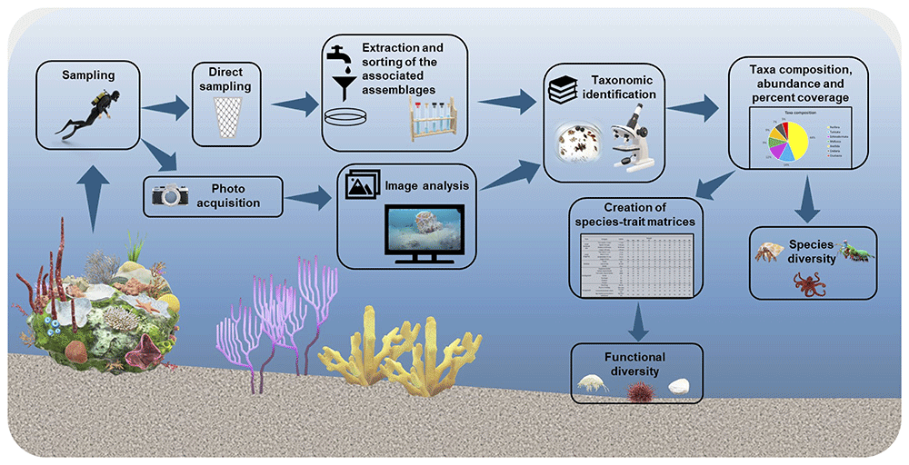
Figure 6. A flowchart representing structural and functional analysis of MAF epibenthic associated assemblages.
In macro-benthic ecology, biodiversity assessment commonly involves multivariate community analysis aimed at characterizing species diversity either within specific sites or across entire ecosystems. In habitats dominated by ecosystem engineer species, such as MAFs, these analyses often focus on the associated epibenthic assemblages, such as coral-dwelling species (Shmuel et al., 2022). This approach has proven valuable in revealing the ecological roles and importance of MAF systems. Numerous studies have investigated the epibenthic communities linked to key habitat-forming species like large bivalves (e.g., Pinna nobilis) (Addis et al., 2009; Cosentino & Giacobbe, 2007; Rabaoui et al., 2009) and gorgonians (e.g., Eunicella gazella, Leptogorgia lusitanica, Isidella elongata) (Camps-Castellà et al., 2024; Carvalho et al., 2014; Cartes et al., 2022; Ponti et al., 2018). These studies consistently demonstrate distinct biodiversity patterns and emphasize the role of ecosystem engineers as promoters of local biodiversity. However, taxonomic analyses alone may not capture the full ecological complexity within and across MAFs. To address this limitation, incorporating functional assessments of epibenthic communities is increasingly recommended. Although still relatively few, studies that combine both structural and functional analyses, such as those examining communities associated with bivalves (Iannucci et al., 2023) and corals (Pitacco et al., 2017), have produced highly informative results, highlighting the potential benefits of this integrative approach across diverse MAF systems. This section offers a concise overview of the most commonly used methods for both structural (uni- and multivariate) and functional analyses.
2.2.2. Methodologies for capturing species diversity
Sampling and sample analysis
1. Sampling: macro-benthic community sampling is usually performed by scientific scuba divers or remotely operated vehicles and typically employs two primary methods, determined by the sampling technique utilized: direct sampling (Bianchi et al., 2004) or indirect sampling through image analysis (Rossi et al., 2021). For direct sampling, regardless of the structuring species, such as massive corals, gorgonians, or bivalves, the associated macrofauna (organisms 500 µm or larger) typically inhabit the surface, interstices, or interior of empty shells. Substrate samples over a standard area (e.g., 20 × 20 cm) can be obtained underwater using a hammer and chisel or steel spatulas and collecting material in synthetic fabric bags; a small airlift device with a mesh bag may help in collecting both scraped sessile organisms and vagile ones. Alternatively, removable short- or long-term recruitment panels can be used to avoid scarification of natural substrates, in some cases also allowing analysis of interspecific interactions (Ponti et al., 2011; Ponti et al., 2014; Ponti et al., 2016) and of infauna and bioeroders (Turicchia et al., 2022). In the laboratory, macrofauna samples require careful rinsing or gentle scraping of the colonized surfaces, with the collected material later passed through 500 µm mesh sieves to isolate the organisms efficiently. In contrast, indirect sampling relies on photographic samples generally performed using digital cameras and proper flashes/lights on a standard area (typically 20 × 20 cm to 1 × 1 m), which is ensured using custom stainless-steel frames. Larger areas can be obtained by photomosaic and even using photogrammetric methods, the latter also capable of providing 3D models (Rossi et al., 2021).
2. Sorting organisms and taxonomic identification: Organisms collected directly from the field are carefully examined under a stereomicroscope for preliminary classification into major taxonomic groups. They are then identified to the lowest possible taxonomic level using morphological characteristics, aided by dichotomous or combinatorial identification keys, and subsequently counted. When morphological identification proves difficult, molecular methods—such as DNA extraction and analysis—can be employed to achieve accurate species identification, provided that reference libraries are available for comparison. For solitary species, abundance is typically reported as the number of individuals per sampling unit or per area (e.g., per square meter). In contrast, for colonial species, metrics such as percent cover, biovolume, or biomass per unit or area are more appropriate. Photographic samples are analyzed using specialized software—such as PhotoQuad (Trygonis & Sini, 2012)—to estimate the percent cover of visually dominant sessile species. Any portions of photographs obscured or rendered unusable (e.g., by foreign objects) should be excluded from analysis, and percent cover values adjusted accordingly. Estimates can also include sediment cover and bare substrate (Ponti et al., 2011; Ponti et al., 2018). For accuracy, percent cover is best assessed through superimposed grids or pixel-counting techniques, which utilize the entire image and offer consistent sampling probability across species of varying sizes and morphologies. In contrast, methods based on a fixed or random set of points resample only portions of the image, potentially biasing species representation and imposing a ceiling on the number of species detected (Ponti et al., 2018). Species identification from photographs can be difficult; hence, morpho-functional units are often used as proxies. Nevertheless, strong knowledge of local fauna and flora, along with access to comprehensive field guides and reference collections linking images to physical specimens, greatly enhances identification accuracy. Emerging artificial intelligence (AI) systems for image-based species recognition are showing promise, especially as they are trained on expanding databases of annotated underwater imagery. The integration of AI with 3D modeling could significantly advance non-invasive sampling methods, particularly in sensitive ecosystems like MAFs (Rossi et al., 2021) and marine reserves.
3. Biomass estimates for secondary production: To better understand the flow of energy and materials within a community, biomass and biovolume measurements are commonly used, as they quantify the organic matter present in both solitary and colonial species. Biomass is typically reported as wet mass (WM), dry mass (DM), or ash-free dry mass (AFDM), with AFDM providing the most accurate estimate of organic content by excluding inorganic components. Following standard procedures, WM is measured immediately after species identification, with surface water removed by gently blotting specimens with absorbent paper. This method provides a consistent baseline for assessing the organic contribution of individual species to community structure and energy dynamics. DM is determined by drying specimens at up to 80°C for at least 24 hours, or until the weight stabilizes, followed by cooling in a desiccator to prevent moisture absorption. For shelled organisms, if only the organic fraction is of interest, soft tissues must be separated from the shell before weighing (Palmerini & Bianchi, 1994), ensuring an accurate measurement of organic content. AFDM is calculated by subtracting the ash mass (AM)—obtained by incinerating the dried sample at approximately 450°C for 8 hours and weighing the remaining inorganic residue after cooling in a desiccator—from the DM. AFDM is often expressed as a percentage of DM (% loss on ignition (LOI), offering a precise indicator of organic matter crucial for evaluating ecological functions. Alternatively, CHNS analyzers can be employed to determine the elemental composition (carbon, hydrogen, nitrogen, sulfur), though they do not directly quantify total organic matter. When available, allometric equations provide a useful alternative for estimating biomass and metabolic rates based on percent cover data, enabling the application of ecological and trophic models (Donati et al., 2024).
Simple measures of species diversity
Species diversity is a key feature of compositional biodiversity at the community level. Many species diversity indices were developed as mathematical measures used to quantify the variety of species within a community (Magurran, 2004). They complementarily consider the species richness (e.g., the number of species S) or the relative abundance of each species (e.g., the Pielou J’ evenness index), or both combined aspects (e.g., the Shannon H’ species diversity, or entropy, index), as a measure of the overall species heterogeneity. There is a growing consensus among researchers to follow the unifying series proposed by Hill (1973), where N0 represents the number of species, N1 (the exponential of the Shannon index) represents the effective number of species (i.e., the number of equally abundant species needed to equal the heterogeneity of the sample), and N10 is the corresponding evenness index.
Diversity indices are typically computed and analyzed according to the experimental design with univariate parametric and non-parametric tests using statistical software such as R (R Core Team, 2024), with packages like vegan (Oksanen et al., 2024) and GAD (Sandrini-Neto et al., 2025), or PRIMER (Clarke & Gorley, 2015), based on species abundance data. These tools provide a robust framework for quantifying and comparing biodiversity in macro-benthic and MAF communities. However, despite the widespread use of these indices, especially for comparative purposes, it is important to remember that they do not provide any qualitative or functional information on the species present.
Community structure analysis
When one wants to analyze the macro-benthic assemblages associated with MAFs, compare them over time and space (beta diversity), and link community structure to environmental variables, it is necessary to resort to multivariate analyses (Anderson et al., 2011; Clarke, 1993; Clarke & Ainsworth, 1993). Starting from the sample-species abundance data matrix, a triangular (dis)similarity matrix among samples is obtained using proper resemblance measures, eventually calculated on monotonically transformed data (e.g., square root, fourth root, log x+1) to balance the effects of rare and abundant species. With a few exceptions, the most suitable similarity measure for abundance data is the Bray-Curtis index (Clarke et al., 2006). Community structure similarities within and between sampling groups can be explored, represented, and analyzed by metric and non-metric bi- and tridimensional ordination plots (e.g., nMDS, PCoA), dendrograms and cluster analysis, multivariate correlation techniques, and tested for differences according to the experimental design with parametric and nonparametric tests (e.g., permutational analysis of variance, PERMANOVA; Anderson et al., 2008).
Functional diversity
Marine functional diversity (MFD) is fundamental to sustaining biodiversity and ecosystem functioning, playing a key role in maintaining the resilience of marine and land–sea interface ecosystems. Over the past few decades, this research area has evolved rapidly, as reflected in the expanding body of primary literature and the increasing number of review articles addressing a wide range of topics and methodological approaches. MFD in macro-benthic ecology and MAFs is commonly assessed using biological traits analysis (BTA). These methods build upon the knowledge of species composition and diversity to select and evaluate the most relevant traits, ensuring they are represented with appropriate types and categories (Carlot et al., 2025). BTA involves the creation of species-trait matrices (e.g., abundance and/or biomass data) that express, for each species, the degree of affinity for a particular trait category. Before calculating functional diversity metrics, the data in species-trait matrices must be normalized. This step ensures that traits with different scales or units contribute equally to the analysis. Once normalized, species-trait data are used to compute various metrics that quantify functional diversity, providing insights into ecosystem processes, species interactions, and resilience. These metrics enable comparisons between different MAF communities, highlighting functional differences and ecological significance.
1. Selection of suitable traits and categories: Selecting appropriate traits and their corresponding categories is a challenging process, as the assignment of affinities to traits often relies on information available in the literature. Generally, BTA incorporates three types of traits: categorical traits (e.g., mobility, living habits); effect traits (e.g., feeding habits); and continuous/response traits (e.g., maximum adult size, longevity, age at sexual maturity). Each trait is further divided into one or more categories. For instance, species in MAF ecosystems can often be characterized by their degree of affinity to these trait categories, enabling a detailed functional analysis of the community. As an example, species living in MAFs can be easily characterized by the degree of mobility, which comprises three categories: sessile, semi-motile, and motile.
2. Assigning degrees of affinity and creating a species-trait matrix: Affinity for traits can be represented using either binary coding (0-1) or fuzzy coding (Chevene et al., 1994). Binary coding indicates minimal (0) or maximal (1) affinity of a species for a trait, while fuzzy coding assigns a more nuanced score ranging from 0 to 3, representing levels of affinity: no affinity (0), low affinity (1), moderate affinity (2), and high affinity (3). Fuzzy coding is generally preferred over binary coding, especially when analyzing communities composed of different taxonomic groups, as it provides a finer resolution of trait differentiation. Conversely, binary coding is sufficient for analyzing single taxonomic groups (Iannucci et al., 2023). It is noted that epibenthic assemblages associated with MAFs are generally characterized mainly by invertebrates such as sponges, crustaceans, various worms’ phyla and mollusks. Sponges show a maximum affinity to the sessile category, so the score would be 1 with binary coding or 3 with fuzzy coding, and a minimum affinity (0) to the motile category, while mollusks show a maximum affinity (1 with binary coding; 3 for fuzzy coding) for the semi-motile category, a low or moderate affinity (1-2 for fuzzy coding) for the sessile category, and a minimum affinity (0) for the motile category. In contrast, crustaceans may express a maximum affinity for the motile category (1 or 3) and a minimum affinity for the semi-motile and sessile categories (0). This methodology is repeated for all traits being analyzed until a comprehensive species-trait matrix is established. The matrix is then merged with abundance or biomass data to facilitate further analysis.
3. Measures of functional diversity: Functional diversity (FD), defined as the diversity of traits within a community, can be quantified through various indices using multivariate and univariate approaches based on normalized abundance or biomass data. Multi-trait approaches, which consider the full range of trait diversity, often rely on dendrogram-based metrics (e.g., Martini et al., 2021; Mouchet et al., 2008; Petchey & Gaston, 2007) or functional space metrics (Laliberté & Legendre, 2010; Villéger & Mouillot, 2008). Functional diversity can be defined by four main metrics, namely functional richness (FRic), functional divergence (FDiv), functional evenness (FEve) and functional dispersion (FDis) (Mason et al., 2005; Murillo et al., 2020; Villéger & Mouillot, 2008). Functional richness measures the extent of trait space occupied by the community; functional divergence defines the predominance of extreme species (with unique trait combinations) and functional differentiation in the trait space; functional evenness describes the extent to which the abundance and/or biomass of a community is distributed within the trait space, and functional dispersion represents the variability and position of species trait groups in the trait space (Villéger & Mouillot, 2008). Single-trait approaches focus on the diversity of individual traits. Metrics such as the community weighted mean (CWM) are valuable for analyzing changes in trait composition. The CWM measures the expected functional trait value in a random community sample and is instrumental in determining functional identity, which reflects the trait strategies driven by the species pool and environmental conditions of a site (Díaz et al., 2007; Iannucci et al., 2023; Pla et al., 2012). For a comprehensive explanation of single-trait and multi-trait metrics, including their mathematical calculations, refer to Pla et al. (2012). These calculations can be performed using species-trait matrices with normalized data and implemented with tools such as the F-Diversity software (Casanoves et al., 2008) or the FD package in R (Casanoves et al., 2011). Relying solely on univariate approaches may provide incomplete insights into the relationships between species abundance or biomass, trait variability, and trait values. To achieve a more thorough and informative assessment of functional diversity, integrating single-trait and multi-trait approaches is recommended.
2.3. Capturing genetic diversity
Techniques such as genetic and genomic analyses, in combination with environmental monitoring and habitat assessments, facilitate the evaluation and documentation of the extensive species diversity, genetic variation, and ecological interactions within marine ecosystems, including MAFs. Understanding ecosystem health is essential for developing effective conservation strategies and enhancing the resilience of marine environments against threats such as overfishing and climate change. Documenting and safeguarding biodiversity is a cornerstone of sustainable marine resource management. To assess genetic diversity, a range of methodologies is available, from basic DNA barcoding to more advanced techniques such as metagenomics, microsatellite analysis, single nucleotide polymorphisms (SNPs), and other omics-based approaches. This paper highlights the most widely used methods for investigating genetic diversity in marine ecosystems.
2.3.1. Use cases for DNA barcoding and species delimitation analysis (SDA)
DNA barcoding, introduced in the early 2000s, employs cytochrome c oxidase subunit I (COI) gene sequences for species identification (Hebert et al., 2003a). This method emerged to address the need for rapid and cost-effective species identification, essential for taxonomy, biodiversity assessment, and conservation. It has since been widely applied to discover new species, resolve taxonomic ambiguities, and complement traditional methods across diverse taxa (Centre for Biodiversity Genomics, University of Guelph, 2021). By using standardized genetic sequences and requiring only small tissue samples, DNA barcoding surpasses traditional morphological methods in speed and reliability (Hebert et al., 2003a; Hebert et al., 2003b). It plays a vital role in biodiversity assessments and monitoring, aiding in cataloging cryptic species and tracking biodiversity loss (Weigand et al., 2019). The use of a standardized genetic marker, such as COI, facilitates consistent comparisons across studies and geographic regions, benefiting conservation and ecological research (Hebert et al., 2003a; Hebert et al., 2003b).
Despite its effectiveness for many taxa, DNA barcoding faces limitations with closely related species, where minimal genetic divergence can lead to misidentifications (Meyer & Paulay, 2005). Its success is also contingent on comprehensive DNA reference libraries. Moreover, technical challenges, such as PCR amplification and sequencing issues, can arise, particularly with complex samples, leading to contamination or amplification biases (Paz & Rinkevich, 2021; Weigand et al., 2019). Nonetheless, DNA barcoding remains a powerful tool for species identification, especially in marine environments, where capturing biodiversity is particularly challenging.
The concept of species is a cornerstone of biodiversity research and biological science. Three primary species concepts are commonly used to identify and understand species: (a) the Biological Species Concept, which defines species based on reproductive isolation; (b) the Morphological Species Concept, which distinguishes species based on observable physical traits; and (c) the Phylogenetic Species Concept, which emphasizes evolutionary relationships and lineage histories. Despite differing approaches, all three concepts share the goal of identifying species, documenting biodiversity, and preserving species before they are lost to extinction. A major challenge in species identification lies in accurately delineating species boundaries and distinguishing between intra- and interspecific variation (Ma et al., 2022; Van Der Bank et al., 2013). SDA refers to the use of biological data to define species boundaries and infer relationships among taxa. SDA supports three key taxonomic tasks: assigning individuals to known species, classifying species into higher taxonomic categories, and describing new species that do not conform to existing classifications. For groups with subtle morphological differences, such as many invertebrates (Ge et al., 2021; Reem et al., 2022) and some vertebrates (Karahan et al., 2017), traditional morphological methods are often insufficient without genetic evidence. In the face of accelerating biodiversity loss, the development of semi-automated SDA approaches that incorporate genomic data offers a practical and efficient solution. While these methods enhance the speed and precision of taxonomic work, they are intended to complement, not replace, the expertise and judgment of taxonomists.
Molecular data used in species delimitation and diversity studies can be obtained from various types of DNA sequences, including single-locus data (e.g., DNA barcoding), multilocus data (such as that generated through techniques like Anchored Hybrid Enrichment [AHE]), and whole-genome data. Phylogenetic approaches, which involve building phylogenetic trees to depict evolutionary relationships, are frequently applied in SDA. Coalescent-based models, such as the multispecies coalescent (MSC) model, evaluate gene tree distributions within the framework of species trees (Rannala & Yang, 2003). Within this context, a variety of algorithms and computational tools have been developed—particularly Bayesian approaches—which enable the modeling of species boundaries and evolutionary relationships using genetic data. Multilocus SDA methods rely on data from multiple genes to define species boundaries more robustly. This paper provides an overview of the DNA barcoding protocol (Figure 7) and introduces a Bayesian framework for single-locus species delimitation (Figure 8).
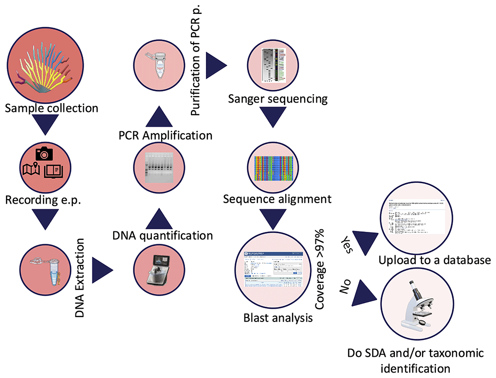
Figure 7. Workflow for DNA barcoding output.
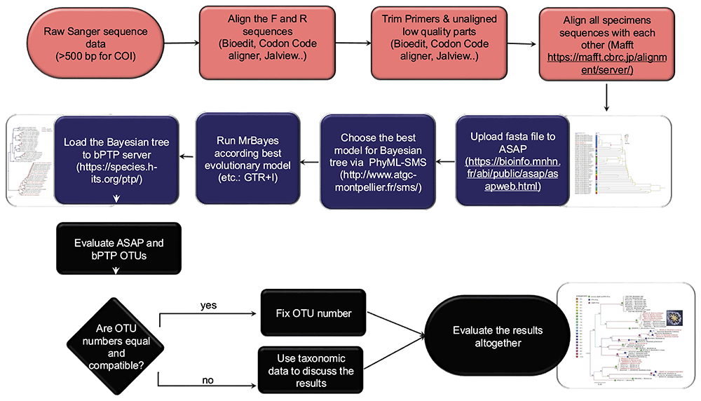
Figure 8. Species delimitation analysis workflow.
2.3.2. Methodologies for DNA barcoding and SDA
1) Sample collection: Take the picture of the whole organism before sampling it with a suitable scale and unique label. Record coordinates and physicochemical parameters. Salinity, pH, temperature, chlorophyll-a, turbidity, dissolved oxygen, and oxygen level observations will help you determine the ecological requirements of your sample. Take the samples as a whole animal (≤0.5 cm), a tissue piece, a colony fragment, etc. Preserving the animal or colony fragment in a formalin solution for taxonomic identification can be helpful if no close match is found at the end of the BLAST analysis. Put the sample in a 1.5 mL vial and label it. Store the samples for at least 24 hrs. in -20°C before DNA extraction. Samples can be stored at -20 or -80°C for a long time (until used for DNA extraction).
2) DNA extraction: Various DNA extraction techniques are available, and selecting the most appropriate method depends on the specific characteristics of the sample. Following extraction, assessing DNA quality is a critical step. Purity is typically evaluated using a Nanodrop spectrophotometer: a 260/280 absorbance ratio close to 1.8 indicates relatively pure DNA, while a 260/230 ratio between 2.0 and 2.2 suggests high-quality nucleic acids. Deviations from these values may indicate contamination by proteins, phenol, or other organic compounds, which can interfere with downstream applications. Ensuring both purity and integrity of the extracted DNA is essential for reliable molecular analyses such as PCR, sequencing, or genomic library construction. Some of the most common DNA extraction techniques are provided below.
a) Phenol-chloroform protocol: One of the best protocols for various MAF species, such as ascidians (Karahan et al., 2022; Paz et al., 2003).
b) CTAB (cetyltrimethylammonium bromide): Originally created for organisms with cellulose cell walls (e.g., plants) but works well for a wide range of MAF species such as corals and ascidians.
c) Chelex: An easy method for DNA extraction, but the DNA loses its integrity very quickly. This method is not ideal for samples collected from protected environments or those not easy to collect.
d) DNA Extraction Kit: Many commercial kits are available that suit the targeted tissue, but a commonly used one is the Qiagen DNeasy Blood & Tissue Kit.
e) Salting-out method: A cost-effective and non-toxic alternative to phenol-chloroform, this method uses high salt concentrations to precipitate proteins, leaving DNA in solution. It has been successfully applied to marine invertebrates, including echinoderms and mollusks (Miller et al., 1988).
f) SDS-Proteinase K protocol: This method uses the detergent SDS to lyse cells and Proteinase K to digest proteins. It's widely used for marine samples with tough tissues, such as sponges and cnidarians, providing high-quality DNA suitable for PCR and sequencing.
3) Amplification of Target Gene Regions: Dilute DNA—Adjust the DNA concentration by diluting with ultrapure water to a final concentration between 10 and 100 ng/µL, which is optimal for PCR amplification. Prepare PCR Reaction—Set up the PCR mix according to your polymerase manufacturer's instructions. Ensure the master mix includes buffer, dNTPs, MgCl₂ (if not pre-mixed), primers, DNA template, and Taq polymerase. Select Appropriate Primers— Choose primer pairs based on your species of interest. For DNA barcoding in marine invertebrates, the mitochondrial COI gene is widely used. Universal primers such as LCO1490 and HCO2198 (Folmer et al., 1994) are a reliable starting point. For higher resolution or species-specific amplification, consider using longer or nested primers or designing species-specific primers based on available reference sequences. Optimize PCR Conditions—Run a PCR program tailored to your primer pair’s annealing temperature and product size. Typical conditions include initial denaturation, 30–35 amplification cycles, and a final extension step. Verify PCR Success—For endpoint PCR, visualize products on a 1.5% agarose gel stained with ethidium bromide or a safe alternative. For qPCR, verify the correct product based on the melting temperature (Tm) curve to assess specificity.
4) Purification of PCR Products: Use a PCR clean-up kit (e.g., ExoSAP-IT™, Qiagen PCR Purification Kit) to remove primers, nucleotides, and enzymes that may interfere with sequencing. Purify the positive PCR products using a PCR cleanup kit (e.g., Applied Biosystems™ ExoSAP-IT™ Express PCR Product Cleanup). After a PCR reaction, purification of the targeted genes is necessary for downstream use, as it helps remove enzymes, nucleotides, detergents, primers, and buffer components.
5) Sequencing of Target Gene Regions: Submit the purified PCR product for bidirectional Sanger sequencing (forward and reverse). This improves accuracy and allows for the correction of ambiguous base calls. Choose a Reliable Sequencing Service—Send your samples to a reputable facility such as Macrogen, Eurofins, or a local genomics center. Ensure you provide primer sequences if not included in the reaction. Post-Sequencing: Check and Edit Chromatograms- Use software such as Geneious, MEGA, or Chromas to inspect chromatograms, trim low-quality ends, and assemble consensus sequences from forward and reverse reads.
6) Data analysis and getting DNA barcodes: After sequencing, follow these steps to analyze your data, generate reliable DNA barcodes, and assign taxonomic identity:
a) Trimming and sequence alignment: Begin by removing the primer regions from your raw sequence reads, as retaining them may lead to reduced alignment quality in subsequent BLAST analyses. Focus on the central, high-quality portion of the sequence. Align the forward and reverse reads to create a consensus sequence using tools such as BioEdit (Hall, 1999), Geneious Prime (http://www.geneious.com/), CodonCode Aligner (CodonCode Co.) UseGalaxy platform (Abueg et al., 2024). After alignment, manually inspect and trim low-quality regions at both ends of the consensus sequence to ensure high accuracy and reduce sequencing errors.
b) Blast analysis for taxonomic matching: Submit the consensus sequences to public databases such as BOLD Systems (Barcode of Life Data Systems; Ratnasingham & Hebert, 2007) and NCBI BLASTn (Basic Local Alignment Search Tool; Johnson et al., 2008). Record the percent identity, which indicates the similarity between your sequence and the reference. Values ≥97% are typically used as a reliable species match. Record the query coverage, which represents the portion of your sequence that aligns to the reference. A minimum of 85% query coverage is recommended. Consider running both BOLD and NCBI BLAST searches for cross-verification of results and higher confidence in taxonomic assignment.
c) Data submission: Submit your sequence to a public database such as BOLD or NCBI, making sure to provide all relevant metadata. This should include detailed information on the sampling location, specimen characteristics, and, when available, a voucher ID linked to a preserved fragment of your sample housed in a museum or research institution. The BOLD system assigns a unique BOLD ID only to sequences that meet minimum quality criteria, typically requiring high-quality, sufficiently long, and unambiguous reads. If your sequence does not meet these standards, you may need to optimize your PCR conditions or repeat the sequencing process. Once accepted, your submission will receive a DNA barcode and a corresponding BOLD or GenBank accession number, which can be cited in future analyses or publications. This step is crucial for building reliable reference libraries and ensuring reproducibility in biodiversity research.
d) Assigning species name: Assign a species name to your sample based on a minimum sequence identity of 97% and a query coverage of at least 85%, as determined by BLAST or BOLD results. These thresholds are generally reliable for many taxa; however, they may vary depending on the group studied. For example, in botryllid ascidians, species-level divergence may exceed 10%, requiring more stringent criteria for accurate identification (Reem et al., 2022). It’s important to note that some sequences in public databases may be incorrectly annotated, so always prioritize references validated by expert taxonomists when resolving ambiguous matches. If your sequence aligns with multiple species, consider the geographic context, ecological data, and morphological traits of your specimen. To further refine identification and validate taxonomic placement, perform SDA, which help define species, genus, or family-level boundaries using genetic data and evolutionary models.
7) SDA protocol—single-locus methods (Figure 8): Species delimitation can be conducted using two main single-locus methods: Automatic Barcode Gap Discovery (ABGD), recently updated as ASAP (Assemble Species by Automatic Partitioning) (Puillandre et al., 2021), and the Poisson Tree Processes (PTP) model (Zhang et al., 2013). ABGD/ASAP identifies species boundaries by detecting barcode gaps in pairwise genetic distances, whereas PTP employs a tree-based coalescent approach, inferring speciation events from branch length patterns. Both methods define Operational Taxonomic Units (OTUs), representing putative species. Although multiple genetic markers can be used in SDA, the mitochondrial COI gene remains the most widely applied MAF species due to its high resolution in many invertebrate groups. Depending on the taxon, additional loci such as nuclear genes (e.g., ITS, 18S rDNA) or chloroplast genes (e.g., rbcL, matK) may be appropriate. For more comprehensive species delimitation, multilocus datasets, including concatenated genes, RADseq, or Ultra-Conserved Elements (UCEs), offer enhanced resolution and accuracy (Erickson et al., 2021). After selecting the marker and completing the PCR and sequencing steps, follow these steps for SDA using a single-locus approach:
a) Editing, alignment, and BLAST search: Edit raw sequences to remove low-quality regions using software such as BioEdit (Hall, 1999), Geneious Prime (http://www.geneious.com/), MEGA (Kumar et al., 2016), CodonCode Aligner (CodonCode Co.), or Jalview (Troshin et al., 2011). Ensure that sequences are properly trimmed and aligned using appropriate bioinformatics tools. Perform sequence alignment with software such as MUSCLE, MAFFT (Katoh et al., 2002), or ClustalW (Thompson et al., 1994). Carefully inspect and manually adjust alignments, especially in regions with indels or ambiguities. Conduct a BLAST search against public databases (e.g., BOLD, NCBI) to compare consensus sequences with known references. Species identification should be based on BLAST matches with ≥97% sequence identity and ≥85% query coverage.
b) DNA barcoding gap analysis: ASAP (Puillandre et al., 2021) is used to detect barcode gaps and suggest species boundaries. Conduct ASAP analysis utilizing the web-based interface accessible at https://bioinfo.mnhn.fr/abi/public/asap/asapold.html#. ASAP provides Jukes-Cantor (JC69), Kimura 2-parameter, and Simple Distance (p-distances) metric options for pairwise distance calculations. Adjust parameters as necessary to fine-tune the clustering process (e.g., distance thresholds).
c) Constructing a phylogenetic tree: Prior to executing MrBayes (Ronquist et al., 2012) to ascertain the optimal model for your data, it is advisable to utilize PhyML-SMS v3 (Smart Model Selection, Lefort et al., 2017) software to identify the most suitable model for your sequence data. PhyML-SMS is a tool designed to identify the optimal model for examining the evolutionary relationships among species, ensuring that the analytical choices are appropriate for the data at hand. For example, the parameters include a marker (COI), a model (GTR+R), and a combined bootstrap of 5,000,000, which is suitable for approximately 600 base pairs of sequence data and around 50 samples.
d) bPTP (Bayesian Poisson Tree Processes) analysis: Use bPTP to model species delimitation on a phylogenetic tree (http://species.h-its.org/ptp/; Zhang et al., 2013).
e) Validation and cross-validation: Cross-validate species boundaries by comparing results obtained from different methods or datasets. Compare outputs from ABGD and PTP to confirm species boundaries and assign OTUs. Ensure consistency with expert-curated reference sequences to minimize the risk of misidentification. Where possible, support molecular findings with morphological, ecological, or behavioral evidence. In cases of conflicting results, consider additional analyses or seek expert consultation.
f) Interpretation of results: Assess whether the delimited species correspond to known taxonomic entities or indicate the presence of cryptic or novel species. Interpret species boundaries in relation to geographical distribution and ecological factors. Explore gene flow and potential hybridization among delimited species using tools such as DNAsp (Rozas et al., 2017). Once boundaries are established, assign species names based on the best sequence match and alignment with known references, taking into account established thresholds and curated databases. If a sequence matches multiple species, conduct further analyses or consult expert taxonomic references to confirm the identification. Present species hypotheses supported by multiple lines of evidence. Document the SDA results, including methodologies, datasets, and conclusions. Share the findings through peer-reviewed publications or public repositories (e.g., BOLD, NCBI) to contribute to broader taxonomic and biodiversity research.
2.3.3. Use cases for environmental DNA (eDNA) metabarcoding
eDNA metabarcoding is an advanced molecular technique used to assess and quantify biodiversity by analyzing eDNA collected from sources like soil, water, and air (Pawlowski et al., 2018). By merging traditional DNA barcoding with high-throughput sequencing technologies, it enables the identification of multiple species within complex biological communities, without the need for direct observation or physical collection of specimens. This non-invasive method is especially valuable for monitoring elusive or rare species, detecting invasive organisms, evaluating ecosystem health, and tracking biodiversity shifts driven by natural or anthropogenic changes. The increasing popularity of DNA metabarcoding in ecological research has brought attention to the need for standardized protocols. Elbrecht & Leese (2015) proposed a systematic workflow that includes key steps such as sample collection, DNA extraction, target region amplification, sequencing, and bioinformatics processing. This structured approach ensures consistency and reliability across studies. Recent applications demonstrate the versatility and effectiveness of DNA metabarcoding. For instance, Thomsen et al. (2012) used the method to monitor marine fish biodiversity, highlighting its advantages over conventional surveys, which can be labor-intensive and less accurate. Likewise, eDNA has proven especially useful in detecting cryptic or low-abundance species often missed by traditional techniques (Bohmann et al., 2014). One of eDNA metabarcoding’s key strengths is its capacity to track temporal changes in species composition, providing insights into the impacts of environmental stressors or habitat alterations (Ogden, 2022; Pawlowski et al., 2018; Suren et al., 2024; Takahashi et al., 2023; Zhang et al., 2023). Research by Jerde et al. (2011) and Nguyen et al. (2020) further supports its utility as a sensitive and efficient tool for assessing biodiversity in both freshwater and marine ecosystems.
Despite certain limitations, such as sequencing errors, contamination from non-target DNA, and incomplete reference databases (Keck et al., 2023), eDNA metabarcoding remains a highly effective tool for biodiversity assessment. Ongoing advancements, including the expansion of comprehensive genetic reference libraries and the refinement of bioinformatics workflows, are steadily improving the accuracy and reliability of this method (Compson et al., 2020; Zhang et al., 2023). Moreover, emerging multi-marker metabarcoding strategies hold promise for revealing more detailed insights into community composition and functional diversity. This paper introduces a standardized eDNA study workflow (Figure 9) and outlines a processing pipeline tailored to various sample types (Figure 10).
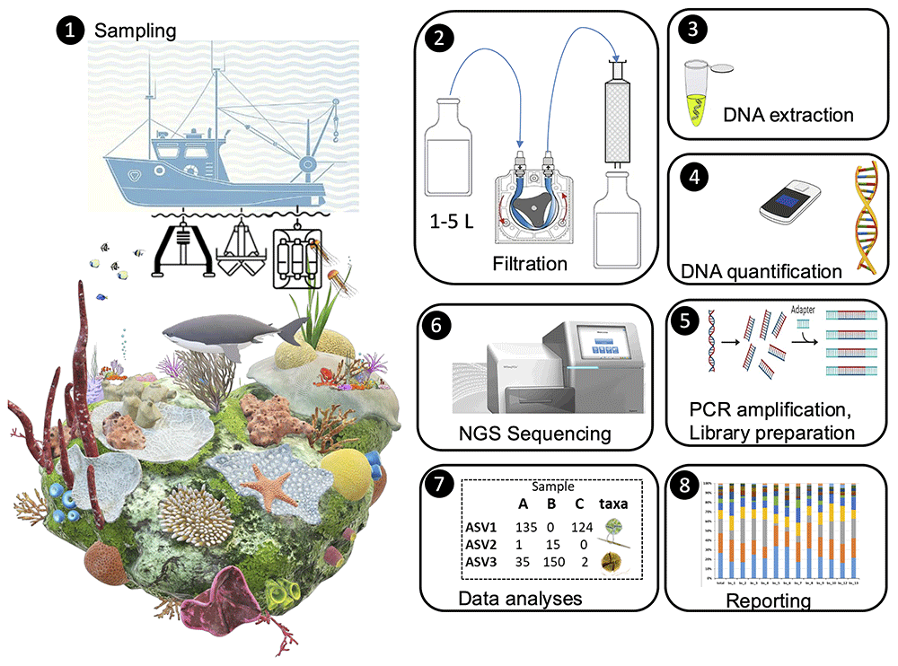
Figure 9. Experiment timeline workflow of an eDNA study.
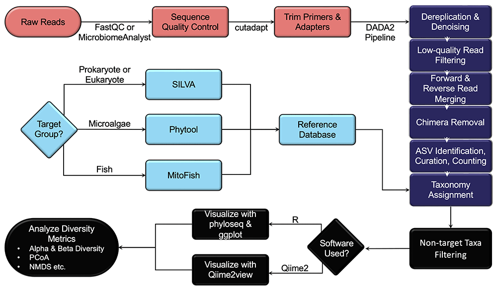
Figure 10. An example flowchart for the bioinformatic analysis protocol of the eDNA metabarcoding.
2.3.4. Methodologies for eDNA metabarcoding
An eDNA study typically progresses through a series of structured steps to facilitate the accurate collection, extraction, and analysis of eDNA, ultimately supporting reliable biodiversity monitoring. The initial phase—Study Design and Sampling Plan—comprises three foundational components: Objective Setting (define the research objectives, such as species detection, biodiversity monitoring, and habitat assessment), Site Selection (choose appropriate sampling locations based on the target species, ecosystem, and environmental conditions), and Sampling Frequency and Replication (plan for multiple time points or replicates to ensure reliable and consistent data). Following these preparatory steps, the study proceeds through the core phases of an eDNA workflow, which are outlined in detail below (Figure 9 and Figure 10):
1) Sample collection: Sterilize equipment and the environment at each step using the following sequence: 10% HCl, 70% ethanol, distilled water, and filtered seawater passed through a 0.2 µm filter. Collect 1–5 L of seawater samples using Niskin bottles from various depths and regions within the sampling site. Replicate each sample (seawater or sediment) at least twice. To collect sediment samples, use a sterile sampler to obtain 0.1–0.2 g of sediment. Ensure that the Van Veen grab is clean before use, and discard any sediment that comes into contact with the equipment. Transfer the sediment into 2 ml sterile tubes using a sterile spatula.
2) Sample filtration: Utilize a vacuum pump or syringe to filter seawater samples using polyethersulfone (PES) or Sterivex filters with a pore size of 0.22 µm. Sample volume may vary based on site characteristics. For larger volumes, pre-filter your water with 0.47 µm filters before using 0.22 µm filters, and use both filters for eDNA isolation. Filtration must be completed within 60 minutes for each sample.
3) Storage: Store filters or sediment samples at -80°C until DNA isolation, or add DNA stabilizers to prevent degradation and store at room temperature.
4) eDNA extraction: Put filters at -20°C for 24 hours; subsequently, bisect each filter to create a replicate. Transfer each filter half into a sterile 0.2 mL centrifuge tube and extract DNA. Extract DNA using the phenol-chloroform protocol (Karahan et al., 2022; Paz et al., 2003) or a commercial kit (e.g., DNeasy PowerWater Kit or DNeasy PowerSoil Pro Kit, QIAGEN). Conduct the extraction in clean, designated laboratories and follow strict protocols to minimize contamination from non-target organisms.
5) eDNA quantification and storage Quantify DNA concentration and quality with a NanoDrop spectrophotometer or a Qubit fluorometer. If DNA quality and quantity are inadequate (< 5 ng/µL), repeat the protocol with the remaining sample or replicate. Store isolated DNA at -20°C until library preparation.
6) Library preparation: Select genetic markers appropriate for target gene regions based on the organisms of interest. Use PCR primers that target variable regions of highly conserved nuclear or mitochondrial genes, such as the V7-V9 region of 18S rDNA (Tanabe et al., 2016) for eukaryotic diversity and the V3-V4 region of 16S rDNA (Herlemann et al., 2011) for prokaryotes. A set of universal PCR primers that target the 12S rDNA gene (Miya et al., 2015, modified from Stoeckle et al., 2022) can be used for fish eDNA metabarcoding. Multiple markers are recommended for comprehensive assessments. Perform PCR amplification of the target genetic region. This process involves amplifying the specific DNA sequences of interest to a detectable level. Ensure that PCR reactions are properly optimized to reduce false positives, contamination, or bias. Negative controls should be included to detect contamination.
7) Next generation sequencing (NGS): Follow a standardized protocol for Illumina MiSeq library preparation and sequencing (paired-end, 2x300 bp). DNA sequencing services may be obtained from either national or international companies (e.g., Macrogen Inc.). Ensure sufficient sequencing depth to obtain comprehensive data, especially for low-abundance species.
8) Bioinformatic analyses (Figure 10):
a) Conduct sequence quality control using FastQC (Andrews, 2010) or MicrobiomeAnalyst 2.0 (Lu et al., 2023). For the bioinformatic analysis pipelines, either R (R Core Team, 2024) or QIIME2 (Bolyen et al., 2019) software can be utilized.
b) Use bioinformatics tools (e.g., QIIME, DADA2, USEARCH) to process the sequencing data, removing adapters, primers, and chimera sequences. Trim primers and adapters with cutadapt (Martin, 2011).
c) Apply the DADA2 pipeline (Callahan et al., 2016) for dereplication, low-quality filtering, read merging, chimera removal, ASV identification, and read counting for relative abundance analysis.
d) Curate and transform the ASV table for ecological interpretation. Prior to ecological analyses, remove low-abundance ASVs and potential contaminants by applying appropriate prevalence or abundance thresholds. Consider prevalence-based filtering (e.g., remove ASVs present in fewer than a given number of samples) and abundance filtering (e.g., remove ASVs below a read count threshold). Normalize the dataset (e.g., via relative abundance or rarefaction) to account for sequencing depth variation among samples.
e) Assign taxonomy using the Assign Taxonomy and add Species functions in DADA2, referencing known databases. Using an appropriate reference database is crucial; it should be reliable and offer high taxonomic coverage of the species. The SILVA database (Quast et al., 2013) is recommended for metabarcoding with 16S and 18S rDNA markers and Phytool v.2 (Canino et al., 2021) for microalgae taxonomy. For fish diversity analysis with the 12S MiFish marker, use the MitoFish database (Iwasaki et al., 2013; Sato et al., 2018; Zhu et al., 2023). The NCBI RefSeq (Sayers et al., 2022) database may also be used to obtain reference sequences; however, additional parameters should be considered to curate and optimize sequences for specific gene regions and organisms of interest.
f) Filter out non-target taxa based on the selected genetic marker. For instance, remove prokaryotic sequences when using the 18S marker or non-fish eukaryotes when using the 12S MiFish marker.
g) Use the phyloseq (McMurdie & Holmes, 2013) package together with the ggplot (Wickham, 2016) package to visualize biodiversity data and analyze diversity metrics, including alpha and beta diversity, PCoA and NMDS graphs, etc. If you use QIIME2, you can visualize bar plots and relative frequency using QIIME2 View (https://view.qiime2.org).
By following these steps, an eDNA study can provide a comprehensive and non-invasive method for assessing biodiversity, monitoring environmental changes, and tracking species populations in ecosystems across a range of habitats.
2.3.5. Use cases for employing microsatellite loci
The below details are constructed following the detailed descriptions in methodological reviews (Glenn, 1996; Rahman et al., 2013; Scribner & Pearce, 2000; Senan et al., 2014). Microsatellites, or Simple Sequence Repeats (SSRs), have been widely used to assess genetic diversity at both inter- and intra-species levels and create genetic and high-resolution linkage maps in various MAFs, including corals (Nakajima et al., 2017; Rachmilovitz et al., 2024a; Rachmilovitz et al., 2024b), ascidians (Dupont et al., 2010; Reem et al., 2023; Tamir et al., 2022), sponges (Salas-Castañeda et al., 2024; Yakhnenko et al., 2024), bryozoans (Freeland et al., 2000; Johnson & Woollacott, 2012), bivalves (Feldheim et al., 2011; Woo et al., 2023), and more. Genome sequencing projects have identified microsatellites in well-studied genomes, which can be applied to related, lesser-studied species with a higher success rate. The polymorphism of SSRs is analyzed through polymerase chain reaction (PCR) due to its advantages over hybridization-based methods. Optimizing PCR conditions and reagent concentrations is essential for successful microsatellite amplification. For studying microsatellites, PCR is used to detect length polymorphisms with specific primers flanking the target regions. Typically, 35 cycles of varying temperature (denaturation at 95°C, annealing at ~50°C, and extension at 72°C) are used for amplification. PCR products are often checked on one percent agarose gels before further analysis on polyacrylamide or agarose gels. Advances in automation and the use of thermostable DNA polymerases have expanded PCR's applications.
Before starting PCR, it’s crucial to optimize conditions for successful amplification of the desired products. PCR conditions tailored to one locus may not work for other microsatellite loci due to differences in primer length and GC content. Without proper optimization, issues like PCR failure, low yield, non-specific amplification, primer-dimers, and errors from misincorporation can arise. Additionally, variations in thermocyclers, PCR tube thickness, and reaction components can affect results. However, PCR conditions, particularly the annealing temperature, optimized for one species can often be applied to another if the same primer pairs are used. Precautions are essential to prevent contamination in PCR. Use ultra-pure water and analytical-grade reagents for all solutions. Proper waste handling and disposal are crucial. To avoid contamination, sterilize the bench surface and always wear gloves while preparing the reaction mixture to prevent contamination from skin cells or hair. Significant contamination usually occurs only when basic preventive measures are neglected. Unless otherwise specified, prepare all solutions at room temperature.
2.3.6. Methodology for employing microsatellite loci
Technical highlights for PCR protocols using microsatellite loci:
1. Microsatellite abundance: Microsatellites are abundant in eukaryotes but in most cases are species-specific.
2. Sample volume: Typically, 20–50 µL per reaction is used, though 10–15 µL is also common. Ensure final reagent concentrations remain consistent. Prepare a pooled master mix and aliquot it into each reaction tube before adding variables.
3. Old PCR machines: For older PCR machine models, add a vapor barrier (e.g., a drop of mineral oil) to prevent evaporation. Mineral oil or glycerol can be used as thermal transfer fluids in the wells.
4. Multiplex PCR: For multiplex PCR, ensure a size difference of more than 20 base pairs between loci to easily distinguish products on acrylamide or agarose gels.
5. Capillary electrophoresis: In capillary electrophoresis systems, use different dyes to improve multiplexing capacity and reduce costs. Most systems can analyze 4-dye chemistry, with some capable of 5-dye chemistry.
6. Impurity dilution: Samples with high levels of impurities, like polysaccharides or phenolic compounds, should be diluted to prevent interference with amplification. If issues persist, use an enhanced DNA isolation protocol with additional steps or chemicals like sorbitol to remove excess impurities.
7. Template DNA: Extract high-quality genomic DNA based on the organism using various methods. Check the quality by running ~50 ng of DNA on a 0.8–1% agarose gel. A bright smear indicates DNA shearing, requiring re-extraction. Quantify DNA using a spectrophotometer (260/280 ratio ~1.76).
8. Taq DNA Polymerase: Available from various suppliers, enzyme concentration in PCR reactions may vary based on formulations and conditions. Note: Different formulations and conditions from various suppliers may result in varying amplification efficiency and intensity. This enzyme is typically used at 1 to 2.5 units per 100 µL reaction.
9. Primers/Oligonucleotides: Design primers based on microsatellite flanking sequences, usually 21–23 bases long with 40–60% GC content. Annealing temperatures should be above 45°C and within 5°C of each other. Dissolve custom-synthesis primers in TE buffer or RNase-free water to create stock solutions, and prepare working concentrations (around 15 ng/µL).
10. Primer concentration: Primer concentration should be optimized for each locus to ensure successful amplification. If PCR products are weak, consider lowering the annealing temperature, increasing the annealing and extension times, raising MgCl₂ concentration, or increasing the number of PCR cycles.
11. Deoxynucleoside Triphosphates (dNTPs): These are essential building blocks for the reaction. They are available individually or as a balanced mixture and are often provided in kits.
12. PCR buffer: A commonly used buffer is 10x [(750 mM Tris-HCl (pH 8.8), 200 mM (NH₄)₂SO₄, 0.1% Tween 20)], often supplied with reaction kits.
13. Magnesium Chloride (MgCl₂): It is crucial for Taq polymerase activity, typically added at 25 mM per reaction. It is usually provided with the kits.
14. Master mix preparation: Multiply the reagent volumes for each reaction by the number of reactions needed to prepare a master mix.
15. Thermal cycler: This machine amplifies DNA by running programmed cycles of temperature changes. Modern thermal cyclers have multiple thermal blocks and heated plates for rapid temperature transitions, and many offer gradient annealing for primer optimization.
16. Water: Use RNase-free water for successful amplification. If unavailable, autoclaved deionized water can be used.
17. Gel visualization: Run PCR products on agarose gel to estimate concentration. Adjust the volume for final gel electrophoresis based on band brightness. For microsatellite allele separation, use 4% high-resolution agarose gels stained with ethidium bromide.
18. Electrophoresis: Test amplification by running PCR products on a 1–1.2% agarose gel stained with ethidium bromide for 30 minutes, followed by polyacrylamide or high-resolution agarose gel electrophoresis.
19. Chelators: Chelators like EDTA in primer stock solutions or template DNA can interfere with optimizing magnesium ion concentration in the PCR mix.
20. Separating PCR reagents: Various methods exist for separating PCR reagents, such as adding Taq DNA polymerase at 72°C, using wax that melts at 75–80°C to mix components, employing antibodies that disassociate above 70°C, using temperature-activated polymerases, or using inhibitors that inactivate polymerase at room temperature.