Introduction
Reducing greenhouse gas emissions is a major challenge in limiting the impact of climate change. Actions, such as energy sobriety, renewable energy generation, and smart energy management, must be undertaken on a large scale. Optimal energy management can be realized by accurately forecasting the energy consumption and production. This implies the need for accurate weather forecasting, and wind speed and solar irradiance evidently play a crucial role in the performance of wind turbines and solar panel energy production, whereas outside air temperature has a notable influence on energy consumption.
The development of weather models requires integration of two critical data inputs: precise weather observations and third-party forecasts.
Weather observations are at the core of modern meteorology and are provided by a range of different methods and tools, such as ground measurements in weather stations, satellite imagery, weather balloons, and radars. This study will use weather observations at ground level; such measurements have been carried out for decades or more in European countries and are currently standardized by the World Meteorological Organization (WMO)1.
The third-party forecast data in this study comprise Numerical Weather Prediction (NWP) data. NWP uses observational data to assess the “current” state of the atmosphere and uses advanced mathematical methods and models based on physical principles to manipulate large and complex sets of data to simulate the future evolution of the atmosphere. Multiple weather providers exist worldwide at different scales (global, regional, local, etc.)2,3. The NWP results are commonly made available on a grid using three dimensions: latitude, longitude, and altitude. The outputs of the model were characterized by their spatial resolution. For example, a resolution of 0,1° corresponds to a square of 15 km (at Borkum latitude). The smallest NWP grid used for the forecast in this study was 0,01°.
The temporal resolution of the NWP result is usually hourly for short-term forecasts, whereas longer-term (several days) forecasts are usually available as 3-hourly or even 6-hourly forecasts.
NWP centers can run various model configurations. Every forecast has a prediction error owing to the complexity of the atmosphere (the system is chaotic), the lack of precision of the observational data and initial conditions, and the inherent model error4.
The aim of this study is to present a method that locally improves existing forecasts from meteorological forecast providers by extending traditional Model Output Statistics (MOS)5 using simple machine learning algorithms. Efforts will be focused on three main weather variables: air temperature (at 2m above ground), wind speed (at 10m above ground), and solar irradiance at ground level.
The authors decided to present a simple prediction method and detail all the steps to achieve accuracy improvement, rather than propose a new complex method. To this end, the reader can easily reproduce this model.
This study selected a set of free-access weather forecasts for the area of interest, followed by a detailed analysis of the forecast data and associated errors. Ultimately, this article details the development of a weather forecasting module that represents the most accurate aggregation of data from these models, thereby improving the accuracy of weather forecasts. This article is related to the “Improved multi-scale forecasting” of the Islander project, H2020 funded project. In the framework of this project, taking place on Borkum, an island in northern Germany, weather forecasting has emerged as a pivotal component of the broader initiative aimed at enhancing multi-scale forecasting capabilities.
Materials and methods
Data acquisition & pre-processing
Data is acquired from 3 APIs made available by the providers:
• ECMWF forecast data is collected through their website1, and access was free of charge in the framework of this European research project.
• DWD observation data is collected through the API or directly on the website2.
• Météo-France forecast data is collected through the API available on their website3.
Data preprocessing is one of the blocks of the overall model. It is necessary to adapt each variable so that models can be compared one to another and applied to the same variables from different sources. It was chosen not to check the quality of the data as an entry point because the quality of observational and forecasted data is very high. For instance, parameters such as the unit and cumulative or instantaneous variables must be homogenized.
• Unit homogenization for air temperature (Kelvin), solar irradiance (W/m2), and wind speed (m/s).
• Transformation to instantaneous values: solar irradiance.
Irradiance values have specificities because the upper limit of hourly values can be restricted in a theoretical manner owing to the clear-sky irradiance6 that, in the first approximation, mostly depends on the position of the sun in the sky. The values of actual ground irradiance can be theoretically capped by the clear-sky irradiance value (in particular, this value is null during night hours).
Clear-sky irradiance was calculated in the model using the pvlib library7. A function that detects when the average irradiance should be zero is coded according to the simulation performed by pvlib.
Wind speed is calculated combining the u- and v- components through the formula:
The last step that has been implemented is filling the missing values in the forecasts. Two methods were successively applied.
• The first method consists of filling holes in a given forecast run by using a simple linear interpolation method. This method only fills “internal” holes in the data (i.e., linear interpolation is used to replace a missing value in a forecast run only if at least one previous and next step values are available).
• The second method, applied after the previous one, consists of using the overlap of successive runs to fill the remaining missing values.
A particular method has been applied to fill missing irradiance values: ECMWF (both for the High Resolution and Ensemble Control models) delivers accumulated forecasts of the solar radiation flux on the ground for each run (the raw variable is accumulated from the start of the run to the end). For medium-to long-term forecasts (lead time higher than +90h), forecasts are only available at a 3-hour or even 6-hour granularity. In this case, the solar radiation flux accumulates over three or even six hours. To fill these gaps, some interpolation methods must be implemented (in particular, to avoid interpreting data as if there was non-null irradiance during night hours). Therefore, it was decided to interpolate the irradiance data by weighting it using theoretical clear-sky irradiance (again computed using the pvlib Python library).
Metric definition
The following metrics from Table 1 are used to compare forecasts and observations of weather variables (with yi being the value of the weather variable and the forecasted value at time i, where n is the number of samples in the considered time series).
Table 1. Definition of the metrics used to assess forecast performance.
| Metric | Formula | Unit |
|---|
| MAE: Mean Absolute Error | | Same as physical parameter |
| MBE: Mean Bias Error | | Same as physical parameter |
| nMAE: Normalized MAE | | % |
| nMBE: Normalized MBE | | % |
These metrics were chosen because they are symmetrical (giving the same importance to positive and negative errors) and MAE and MBE have the added advantage of having the same unit as the physical variable of interest. Here, a positive MBE means that the forecast overestimates the observations, whereas a negative MBE indicates an underestimation.
The normalized versions are computed by dividing the MAE and MBE by the average value of the weather observations; for solar irradiance and (absolute) wind speed, there is absolutely no issue because both parameters are positive. For temperature, on the other hand, working in degrees Celsius implies possible negative values (and an average close to zero so that the normalized errors may “explode” towards very high values). The hourly mean temperatures in Borkum are mostly positive. The nMAE was preferred to the Mean Absolute Percentage Error (MAPE) because all studied weather parameters may take values equal to or close to zero.
Data analysis
In this section, a comparison of the available third-party NWP forecasts (two forecasts from Météo-France and two from ECMWF) with the actual measurements made at DWD weather stations on Borkum Island (or the neighboring Norderney Island for irradiance measurements) is performed. Details of the forecast horizons and granularities are displayed in Table 2.
Table 2. Details of the forecast horizons and granularities for each run of NWP forecasts used in this study.
| | Runs and their horizons (all values in hours) |
|---|
| Models | 00h (UTC) | 06h (UTC) | 12h (UTC) | 18h (UTC) |
|---|
| Météo-France | AROME | 0 to 48 by 1h-steps | 0 to 42 by 1h-steps | 0 to 42 by 1h-steps | 0 to 36 by 1h-steps |
| ARPEGE | 0 to 102 by 1h-steps | 0 to 72 by 1h-steps | 0 to 114 by 1h-steps | 0 to 60 by 1h-steps |
| ECMWF | ECMWF High resolution | 0 to 90 by 1h steps
93 to 144 by 3h steps
150 to 240 by 6 h steps2 | 0 to 90 by 1h steps1
| 0 to 90 by 1h steps
93 to 144 by 3h steps
150 to 240 by 6 h steps2 | 0 to 90 by 1h steps1 |
| ECMWF Ensemble control | 0 to 90 by 1h steps
93 to 144 by 3h steps
150 to 360 by 6 h steps2 | 0 to 90 by 1h steps
93 to 144 by 3h steps | 0 to 90 by 1h steps
93 to 144 by 3h steps
150 to 360 by 6 h steps2 | 0 to 90 by 1h steps
93 to 144 by 3h steps |
This comparison on a historical dataset is made subtle because of the problem of dissemination delay, that is, the time lag between the instant the NWP run is launched and the (later) instant in time when it is made available to users Table 3. For instance, Météo-France launched an ARPEGE run at 00h (UTC) to forecast the evolution of weather until 102 h later (4 and 6 h). However, the results of this run were only made available approximately 3 to 4 h later4. There were three main consequences.
Table 3. Details of the dissemination times for each run of NWP forecasts used in this study.
| | Runs and their real-time availability (UTC time) |
|---|
| Model | 00h | 06h | 12h | 18h |
|---|
| Météo-France | AROME | 02h45 | 11h10 | 15h55 | 23h10 |
| ARPEGE | 03h50 | 10h35 | 15h25 | 22h35 |
| ECMWF | ECMWF High resolution2 | 6h55 | 12h121 | 18h55 | 00h121 |
| ECMWF Ensemble control2 | 07h20 | 12h52 | 19h20 | 00h52 |
• The first few hours of a forecast run can NOT be used under the operational conditions. (For instance, the 00h run from ARPEGE is made available at 3h50 UTC therefore, the forecasts for hours 0 to 3 are not actually usable.)
• The dissemination time reduces the maximum time horizon of a forecast. (For instance, the 00h run of the ARPEGE model forecast has a useful horizon of 98 h instead of 102.)
• The actual time horizon of the forecast must be corrected based on dissemination time. (For instance, the forecast of the 00h run from ARPEGE for hour 13 is made available 9 h before and not 13 h before).
Consequently, a comparison between the measurements and forecasts of weather parameters can be made using two approaches:
1. The first approach is to use a historical forecast dataset “as is” (not taking the dissemination time into account) and therefore evaluating the forecast error in an “ideal” scenario. This method is not fully relevant for operational configuration but may still provide interesting information about the forecast by providing a sort of lower bound for the forecast error.
2. The second approach consists of transforming the forecasts by considering the dissemination time by delaying the runs and removing values that are not actually available.
In this report, except when stated otherwise, method 2 is always applied as it allows the evaluation of the model performances “as if” they had been used in operational conditions. Illustrations depicting the process are shown in Figure 1.
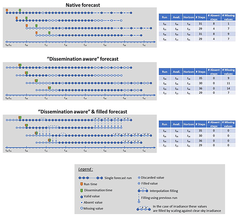
Figure 1. Schematics illustrating the forecast transformation and filling methods that have been implemented.
Weather module development
Global package
The weather Advanced Weather Forecasting (AWP) package was developed in Python. The objective of the module developed is to improve the accuracy of three variables, namely irradiance, temperature, and wind speed, on a 7-day horizon and hourly granularity, and run for three years without interruption.
To address this need, the package has a double functionality: the first is for calibration. It aims to analyze the data and calibrate the model to determine the optimal hyperparameters and parameters. The second purpose was to run the model operationally daily. These two purposes do not require the same functionalities; however, many developments are relevant for both the approaches.
Figure 2 shows the functionalities developed for the operational pipeline. It was built as a combination of multiple units that operate operationally.
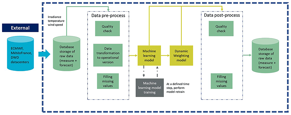
Figure 2. Macroscopic view of the weather package with the pre-process, model and post-process units.
• An import block where data are collected from the database. An overview of the functionality of this block is presented in section 0.
• A pre-process block in which data is cleaned and filled.
• Model block where the forecast is calculated. The main objective of this module is described in detail in the following section.
• A post-process block is used to check if the data published are correct and fill in if the missing data are required.
The other functionalities built for the calibration purpose are:
• A data analysis block, in which the data were analyzed using statistical and visualization methods. It concerns both raw and forecasted data.
• A model calibration block, where all parameters and hyperparameters are chosen, and the models are trained.
Models
Two complementary approaches have been developed for this purpose. The main development is focused on a machine-learning approach, as it is a commonly examined method in the literature, and the results are promising8. The other is a dynamic weighting method that learns from the most recent observational data to improve prediction.
The objective of the Machine Learning module is to deliver a 7-day ahead forecast of the hourly mean of three weather parameters listed before (temperature at 2m, wind speed at 10m and solar irradiance at ground level). To this end, a history of observations and forecasts for these three variables (and many others such as pressure and humidity) has been collected, which is a supervised learning problem, and regression models will be trained (that will predict a continuous variable).
The extended forecast window (from +0 to +168h) is quite challenging, as the methods to address different horizons strongly vary in this range. For instance, in the case of solar irradiance forecasting, different methods must be applied depending on the temporal and spatial resolutions of the forecasts9.
• Persistence methods and time-series models (autoregressive, moving average, and their declinations: ARMA, ARIMA, etc.) are used for very short term (sometimes called “nowcasting”) and short-term forecasting10.
• Other statistical methods (artificial neural networks for instance) are available for medium-term forecasts11.
• For a longer term (and lower spatial resolution), NWP methods are required, but can be refined locally using Model Output Statistics (MOS) methods (see, for instance12, for an example of MOS applied to wind speed forecasting).
In this work, several approaches have been combined to rely on both in-situ measurements and third-party NWP forecasts to make predictions on the full 7-day horizon. This Machine Learning approach will therefore be very similar to an MOS method with the additional benefits of (i) using several (and partly independent) NWP forecasts simultaneously and (ii) adding information from in-situ measurements that should help improve forecasts in the short-term range.
For each of the three variables of interest, the same two-step method is adopted as showed in Figure 3; in phase 1, we use all data available from September 2018 to December 2021 (around 28 months of data) as the training set to tune the model hyperparameters. The performance was evaluated on a validation set containing all the data from 2021. The best combinations of models and hyperparameters will then be selected and phase 2 will be applied where the training set will span September 2018 to December 2021 (approximately 40 months), and the forecast performance will be evaluated on the test set for the first six months of 2022.
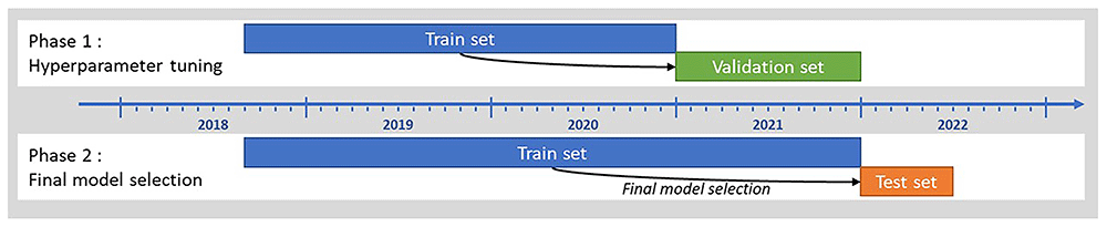
Figure 3. Schematic showing the train, validation and test sets used for the Machine Learning model selection.
The models that were tested in this study mostly come from the scikit-learn python package13, as well as the XGBoost package14.
The Table 4 below shows the details of the modelling aspects and hyperparameters that were tested in Phase 1.
Table 4. Details of the modelling aspects and hyperparameters tested.
| “Hyperparameters” | Tested ranges or instances |
|---|
| Model type | • Linear regression
• Support Vector Machine regressor (with linear kernel)
• Random forest regressor
• Multilayer perceptron
• Gradient boosted decision trees |
| Hyperparameters of the model | • Depends on the model type (e.g. number of hidden layers and neurons in ANNs, maximal tree depth for decision trees, etc.) |
| Input features | • NWP forecasts from third parties (different variables are used, not only the forecast of the variable of interest)
• In-situ measurements (last values available at each time)
• “Calendar” features (hour of day, month of year, etc.) |
| Horizon range | • Full horizon [+0 to +168h]
• Split days (one model predicts hours of the 1st day-ahead, a second model hours of the 2nd day-ahead, etc.)
• Other arbitrary splits |
For phase 2, up to three models (for each of the three variables of interest) were selected for final testing. The chosen models to be confronted were chosen according to their performance on the validation dataset with particular attention to avoid models that tend to overfit data (this tendency is evaluated by comparing the performance metric on the validation and training datasets).
Dynamic weighting integration is common practice in the field of temporal series forecasting. It allows the combination of multiple forecasts by assigning them a specific weight according to their most recent performance15.
The Dynamic Weighting strategy takes advantage of observational data measured on-site in the previous hours. If some of the weather forecast models perform better than the others, it is likely that they will be similar for the next hours10.
The coefficient of each variable is calculated by:
where dwj,k is the weight for each variable k of model k and is inversely proportional to the performance measured Pj,k. Pj,k is calculated as follows:
where Fi,j,k is the forecast of variable k at time i from NWP model j, Oi,k is the observation value of variable k at time i, and N is the size of the comparison.
Finally, the new forecast is calculated as follows:
N, the number of hours for which the performance is measured, is a hyperparameter. According to the literature, 6 h provides a better performance10. This parameter was investigated in the present study.
The dynamic weighting method was applied to five forecast sources: Arome, Arpege, ECHR, ECEC, and the output of the machine learning model.
Results & discussion
Machine learning approach
After a careful selection process, the models chosen to predict each variable are listed in Table 5, as they showed the best performance on the test set (as a reminder for the 6 first months of 2022) in terms of MAE.
Table 5. Selected ML models to forecast the 3 variables of interest.
| Predicted variable | Final model type |
|---|
| Air temperature at 2m, measured at the Borkum Flugplatz | Multilayer perceptron |
| Wind speed at 10m, measured at Borkum Süderstrasse weather station | Multilayer perceptron |
| Solar irradiance at ground level, measured at Norderney weather station | Support Vector Machine Regressor |
Air temperature
Table 6 compares the forecasting performance of the selected Machine Learning model (as a reminder of a Multilayer Perceptron regressor from the scikit-learn package) to predict air temperature at 2m above ground on the Borkum Flugplatz weather station using four different external NWP predictions as well as in situ weather measurements. The models were compared on a dataset comprising the first 6 months of 2022.
Table 6. Machine learning forecast performance for air temperature at 2m compared to 3rd party NWP models: (a) average performance over the whole datasets (6 first months of 2022) (b) one-to-one comparison on identical datasets.
| Provider: | Météo-France | ECMWF | This study |
| Model: | AROME | ARPEGE | HRES | ECEC | ML |
| MAE (°C) | 0.85 | 1.18 | 1.44 | 1.31 | 1.07 |
| MBE (°C) | -0.25 | -0.05 | -0.21 | -0.21 | 0.13 |
| nMAE | 10.2% | 14.3% | 17.4% | 15.8% | 13.0% |
| nMBE | -3.0% | -0.5% | -2.5% | -2.5% | 1.5% |
| Counts | 23 740 | 53 537 | 43 988 | 90 641 | 632 121 |
| Avg. lead-time (h) | 18.0 | 43.9 | 68.0 | 70.3 | 83.1 |
| Provider: | Météo-France | ECMWF |
|---|
| Model: | AROME | ARPEGE | HRES | ECEC |
|---|
| MAE (°C) | 0.85 | 1.18 | 1.42 | 1.29 |
| MAE ML model (°C) | 0.75 | 0.83 | 0.96 | 0.97 |
| MAE improvement1 | -12% | -30% | -32% | -25% |
| MBE (°C) | -0.25 | -0.04 | -0.20 | -0.20 |
| MBE ML model (°C) | 0.15 | 0.15 | 0.15 | 0.15 |
| MBE improvement1 | -40% | +259% | -23% | -28% |
| Counts | 23 498 | 52 793 | 43 185 | 88 997 |
| Avg. lead-time (h) | 18.0 | 43.8 | 67.8 | 70.0 |
The top table compares the performance on the full dataset available for each forecast (reminder: for Météo-France and ECMWF forecasts there are only 2 or 4 runs per day, while the ML forecast has been run in “simulated operational conditions” 24 times a day). The MAE and MBE of the models are, on average, of the same order of magnitude as the NWP forecasts. However, a one-to-one comparison (as shown in the bottom table of Table 6) demonstrates that the ML model performs better than the NWP on identical datasets, with a (relative) improvement of 12% in the MAE compared to AROME (i.e., for short-term forecasting) and up to 32% compared to the high-resolution model from the ECMWF. In terms of bias, the ML model performs better than all NWP models, except ARPEGE, which has a very low MBE.
Graphs available on Figure 4 allow to go into more details in the comparison. As a function of the lead-time, it is observed that the ML model outperforms all NWP predictions.
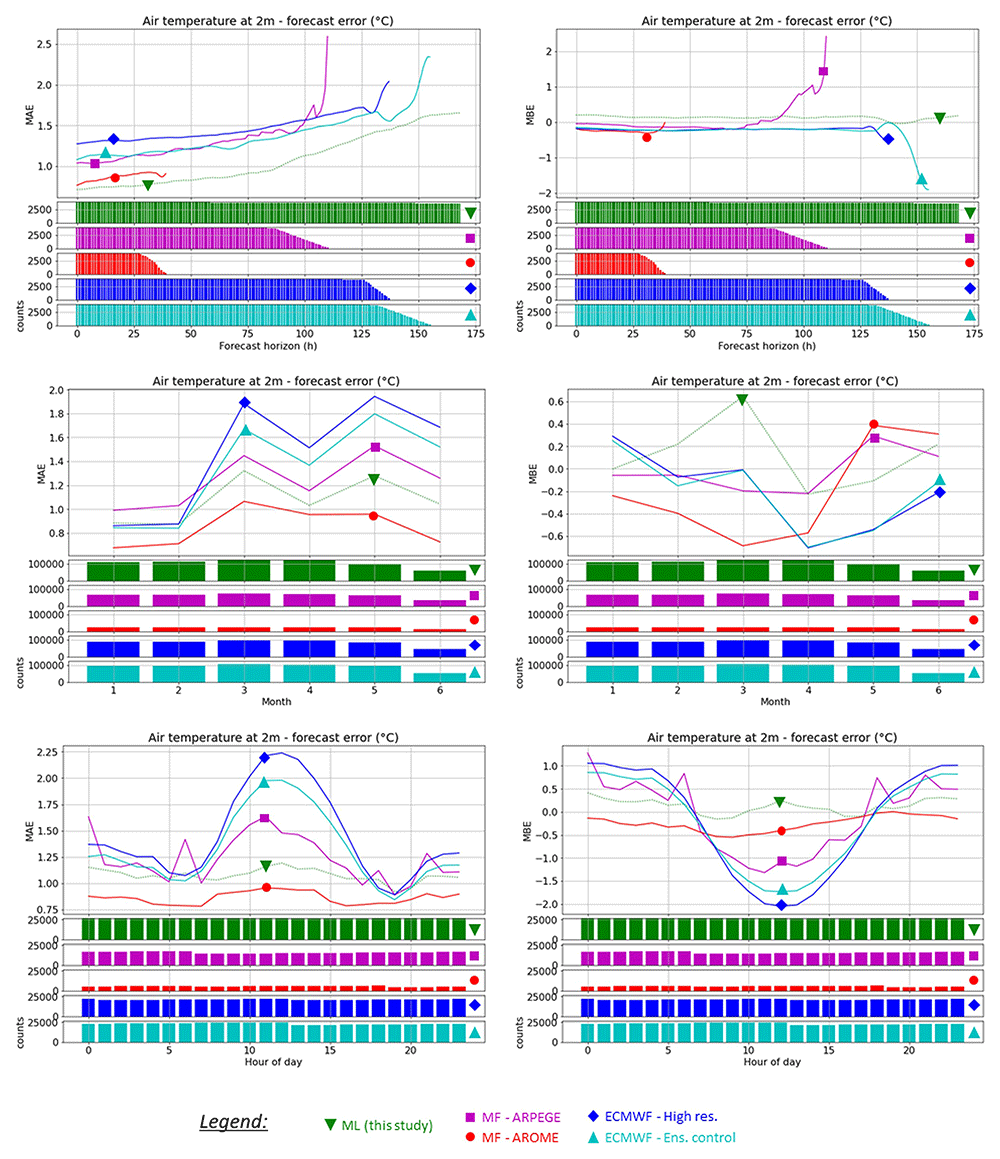
Figure 4. Comparison of the average prediction error for the air temperature at 2m on the Borkum Flugplatz weather station for the four available NWP forecasts and this study’s best machine learning model, period Jan to June 2022, as a function of: forecast horizon (top), month (middle), hour of day (bottom).
Notice that a smoothing method has been applied to the results of the NWP results to better compare the performance as a function of the lead-time.
The monthly behavior does not show any particular pattern; therefore, the ML model seems to perform evenly throughout the year. As a function of the hour of day, the ML model was able to alleviate the daily performance pattern of the NWP forecasts (most evident for ARPEGE and both ECMWF models), and the ML model was able to maintain a similar performance throughout the day.
Solar irradiance
Table 7 compares the forecasting performance of the selected Machine Learning model (as a reminder of a Multilayer Perceptron regressor from the scikit-learn package) to predict solar irradiance at ground on the Norderney weather station using four different external NWP predictions as well as in situ weather measurements. The models were compared on a dataset comprising the first 6 months of 2022.
Table 7. Machine learning forecast performance for solar irradiance at ground level compared to 3rd party NWP models: (a) average performance over the whole datasets (6 first months of 2022) (b) one-to-one comparison on identical datasets.
| Provider: | Météo-France | ECMWF | This study |
| Model: | AROME | ARPEGE | HRES | ECEC | ML |
| MAE (W/m²) | NA | 78.15 | 85.81 | 85.63 | 82.47 |
| MBE (W/m²) | NA | -0.61 | 9.53 | 7.01 | 11.10 |
| nMAE | NA | 29.5% | 32.4% | 32.4% | 31.2% |
| nMBE | NA | -0.2% | 3.6% | 2.6% | 4.2% |
| Counts | NA | 27 272 | 23 604 | 48 337 | 338 561 |
| Avg. lead-time (h) | NA | 41.9 | 68.2 | 70.0 | 83.2 |
| Provider: | Météo-France | ECMWF |
|---|
| Model: | AROME | ARPEGE | HRES | ECEC |
|---|
| MAE (m/s) | NA | 77.76 | 84.94 | 84.99 |
| MAE ML model (m/s) | NA | 68.08 | 77.31 | 77.51 |
| MAE improvement1 | NA | -12% | -9% | -9% |
| MBE (m/s) | NA | 0.22 | 10.02 | 7.07 |
| MBE ML model (m/s) | NA | 2.17 | 3.12 | 4.62 |
| MBE improvement1 | NA | +868% | -69% | -35% |
| Counts | NA | 26 855 | 23 090 | 47 295 |
| Avg. lead-time (h) | NA | 41.7 | 67.8 | 69.7 |
The results obtained for irradiance are very similar for the ML model compared to the NWP forecasts; in terms of MBE, they are even slightly worse on average (as seen in the top graph). In the one-to-one comparison, it appears that a slight improvement in the MAE is achieved by the ML model (9 to 12% relative improvement in the MAE compared to the NWP forecasts). In terms of MBE, the ML model performed better than both ECMWF models; however, the ARPEGE model had a very low bias so that the ML model was considerably worse.
As shown in Figure 5: the ML model clearly outperforms the NWP models in terms of MAE, as well as for the MBE for lead-times below +85h. It can also be seen that the high positive average bias of the ML model (as computed in Table 7) mostly comes from a large overestimation of the irradiance for long-term forecasts.
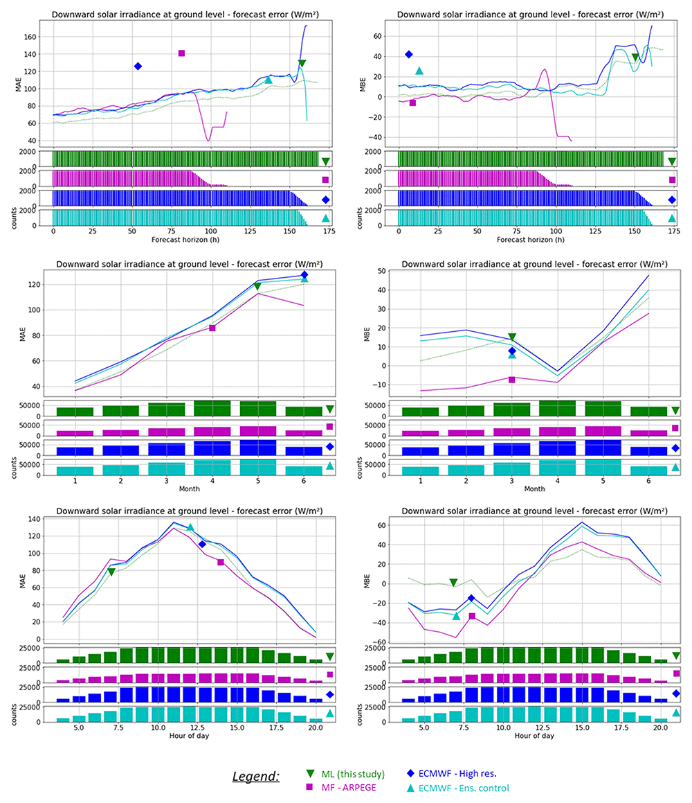
Figure 5. Comparison of the average prediction error for the downward solar irradiance at ground level on the Norderney weather station for the four available NWP forecasts and this study’s best machine learning model, period Jan to June 2022, as a function of: forecast horizon (top), month (middle), hour of day (bottom).
Notice that a smoothing method has been applied to the results of the NWP results to better compare the performance as a function of the lead-time.
The monthly and daily patterns of the ML model are very similar to those of the NWP models; the only important difference is the lower MBE of the ML model in the morning hours.
Wind speed
Table 8 compares the forecasting performance of the selected Machine Learning model (as a reminder a Support Vector Machine regressor from scikit-learn package) to predict wind speed at 10m above ground on the Borkum Süderstrasse weather station using four different external NWP predictions as well as in-situ weather measurements. The models were compared on a dataset comprising the first 6 months of 2022.
Table 8. Machine learning forecast performance for wind speed at 10m compared to 3rd party NWP models: (a) average performance over the whole datasets (6 first months of 2022) (b) one-to-one comparison on identical datasets.
| Provider: | Météo-France | ECMWF | This study |
| Model: | AROME | ARPEGE | HRES | ECEC | ML |
| MAE (m/s) | 1.45 | 2.09 | 2.35 | 2.00 | 1.42 |
| MBE (m/s) | 0.49 | 1.63 | 1.80 | 1.25 | -0.17 |
| nMAE | 23.5% | 33.9% | 38.0% | 32.5% | 23.0% |
| nMBE | 7.9% | 26.5% | 29.2% | 20.2% | -2.7% |
| Counts | 23 657 | 53 355 | 43 838 | 90 330 | 631 952 |
| Avg. lead-time (h) | 18.0 | 43.9 | 68.0 | 70.3 | 83.1 |
| Provider: | Météo-France | ECMWF |
|---|
| Model: | AROME | ARPEGE | HRES | ECEC |
|---|
| MAE (m/s) | 1.52 | 2.16 | 2.40 | 2.07 |
| MAE ML model (m/s) | 0.97 | 1.12 | 1.29 | 1.32 |
| MAE improvement1 | -36% | -48% | -46% | -36% |
| MBE (m/s) | 0.49 | 1.64 | 1.81 | 1.26 |
| MBE ML model (m/s) | -0.21 | -0.21 | -0.22 | -0.23 |
| MBE improvement1 | -58% | -87% | -88% | -82% |
| Counts | 23 568 | 52 972 | 43 323 | 89 272 |
| Avg. lead-time (h) | 18.0 | 43.8 | 67.8 | 70.0 |
As shown in the top table, the ML model for wind speed forecasting performed better than all NWP forecasts, even when comparing the full available datasets, both in terms of MAE and MBE. In the one-to-one comparison available in the bottom table, it is shown that on similar datasets, the ML model performs 36% (relative) better than the AROME and ECMWF Ensemble control models, and almost 50% better than ARPEGE in terms of MAE. The average bias is much lower for the ML model (which slightly underestimates the wind speed, while all NWP forecasts overestimate it).
The graphs in Figure 6 provide a detailed comparison of the ML model performance with the NWP forecasts. The ML model outperformed all NWP forecasts in terms of both MAE and MBE, showing the very high potential of the proposed method for this particular variable. No particular pattern arises as a function of the month, and for the behavior of the forecast as a function of the hour of the day, it is clear that the ML model is able to alleviate the daily pattern of the ARPEGE and ECMWF models (which perform clearly better in the middle of the day compared to the night).
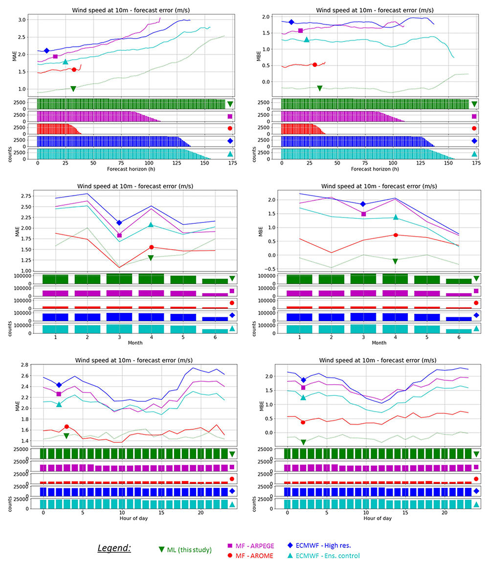
Figure 6. Comparison of the average prediction error for the wind speed at 10m on the Borkum Süderstrasse weather station for the four available NWP forecasts and this study’s best machine learning model, period Jan to June 2022, as a function of: forecast horizon (top), month (middle), hour of day (bottom).
Notice that a smoothing method has been applied to the results of the NWP results to better compare the performance as a function of the lead-time.
Dynamic weighting approach
In the dynamic weighting method, one hyperparameter must be optimized to improve the results, that is, the number of hours in the past on which the mean model performance is calculated. The impact of the number of hours was estimated by 14, which considered that the past 6 h yielded better results. This parameter was tested for the three variables of interest. The optimal hyperparameter was chosen for a lower MAE obtained for the tested dataset. The tests were performed on data collected from 01-01-2021 to 31-12-2021. The dynamic weighting approach was efficient in improving model accuracy only for the temperature variable for the horizon of 48 h because the model performance of the variables was quite similar (Figure 7). On the contrary, this method did not improve the wind speed metric, as one model was significantly better than the other models (nMAE=29% versus nMAE=39%); dynamically mixing models that have significant performance differences on average will not improve the performance as the poorly performing models will always hinder the weighted mix.
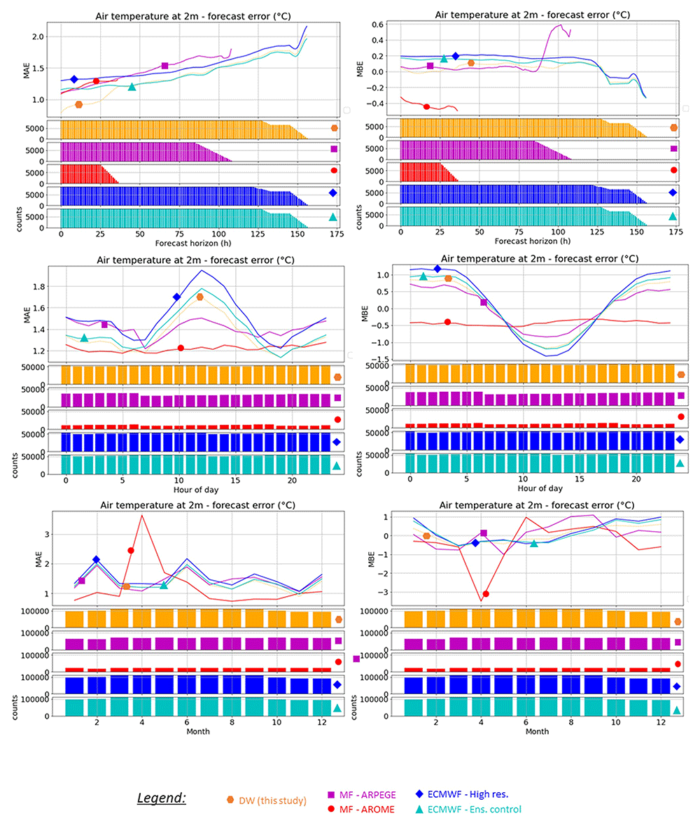
Figure 7. Plot of the MAE (Mean Absolute Error) of the 5 forecasts: MFAO: Météo-France – Arome; MFAP: Météo-France Arpège; ECEC: ECMWF Ensemble Control and ECHR: ECMWF High Resolution and DW06: Dynamic Weighting model with n last hours = 6 considering the time, month, and hour of the day.
Conclusions
This study describes and analyzes a forecasting system to locally improve NWP predictions on the island of Borkum, Germany, in the framework of the European Islander research project. Several machine learning models have been developed and tested on three main weather variables: irradiance at ground level, air temperature 2 m above ground, and wind speed 10 m above ground. Our study shows that a significant improvement in the forecast accuracy can be obtained throughout the forecast horizon (seven days with hourly granularity) for each of the studied variables.
First, a Machine Learning approach with relatively simple models was applied to improve the forecasting of the three variables of interest, using the forecasts of four NWP models and real-time in situ measurements (as well as additional time features) as inputs. After a cautious selection, the final models used to forecast the variables were two different multilayer perceptrons (neural networks) to predict air temperature and wind speed, while a support machine vector regressor was used to forecast the irradiance. A very high improvement in the forecast performance was obtained for wind speed (by 35 to almost 50% in terms of MAE), while the ML models for irradiance and air temperature show a more modest improvement in the forecasting performance (by 12 to 30% in terms of MAE for the temperature and approximately 9 to 12% improvement for the irradiance).
The dynamic weighting approach shows promising results for the temperature variable on short-term horizons (48 h), but it does not considerably improve the accuracy of wind speed and irradiance variable forecasting, most probably because the considered NWP models have too high average performance differences so that their (weighted) average will always underperform compared to the best one.
Patents
Ethics and consent
Ethical approval and consent were not required.








