Introduction
Approximately 10% of the market share for robot applications is attributed to the plastics and chemicals industries, notably in reducing unit costs and improving competitiveness over the past decades1. The growth is anticipated to be propelled further as flexible robots with programming capability to enable the integration of downstream automation. Integrated robot-machine systems not only offer advantages in floor space and cycle time but also facilitate long periods of unattended operation, contributing to the industry's continued evolution2. The injection moulding industry is a major user of robotic applications in the plastics industry, which has witnessed significant growth in robotic utilisation, from unloading injection moulding machines to material handling, machining, and material deposition.
Compared to injection moulding, rotational moulding, or rotomoulding, is a more straightforward process for producing plastic mouldings. However, rotational moulding faces a considerable technical lag that requires catching up to match the advancements seen in injection moulding3. Originating in the late 1950s with PVC plastisol moulding, it primarily involves polyethylene (PE) and stands out as a niche in the plastics industry. Despite its relatively small share, rotational moulding exhibits above-average growth rates, offering design flexibility for products ranging from bulk storage containers to intricate automotive, medical, and aerospace applications. The process, known for producing hollow, complex forms, is gaining recognition for intricate parts like fuel tanks and aircraft components. Market trends favouring component consolidation and shorter product life cycles elevate its significance, drawing major material suppliers' attention and development efforts, which play a pivotal role in the industry's future development4.
A typical rotational moulding process is illustrated in Figure 1. The basis of the process is heating and tumbling the polymer powder within a heated mould. The polymer powder becomes sticky and adheres to the inside of the mould surface to form the designed shape. Following that, the mould undergoes a cooling process, causing the polymer to solidify and create a hollow product. Once the product is removed from the mould, it typically requires minimal to no post-processing, which could include de-flashing, trimming, drilling or assembly5. Therefore, almost 100% of the raw material turns into the final product, making it a very effective and economical way to manufacture hollow plastic products, especially for large and small batch products.
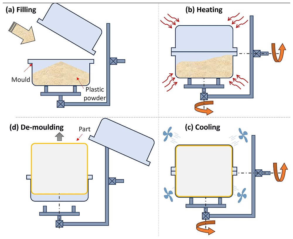
Figure 1. Typical moulding process for rotational moulding.
The Internal Air Temperature (IAT) has long been established as a critical parameter overseeing the moulding process and determining the properties of the product6. The heating and cooling cycle in rotational moulding (Figure 2) involves the plastic powder adhering to the mould from Point A. Then, the IAT increase slows as the plastic melts and absorbs extra heat, continuing until Point B when all plastic adheres to the mould. A loose powdery mass, formed by sticky plastic powder adhered to the mould, undergoes sintering and densification in region BC, forming a uniform melt. There is a noticeable temperature rise for the IAT after the mould is removed from the oven before it drops, attributed to the residual heat in the mould metal. At Point D, a significant slope change marks the solidification of the plastic, releasing heat. Once solidified across the wall section, the internal air temperature decreases, usually more slowly than before solidification due to a poorer heat transfer rate in solid form. The final stage, Point E, shows a slight slope change, indicating the plastic separates from the mould, forming an insulation layer of air between them. This reduces external cooling efficiency, slowing the internal air temperature decrease. Eventually, the demoulding temperature is reached at Point F7.
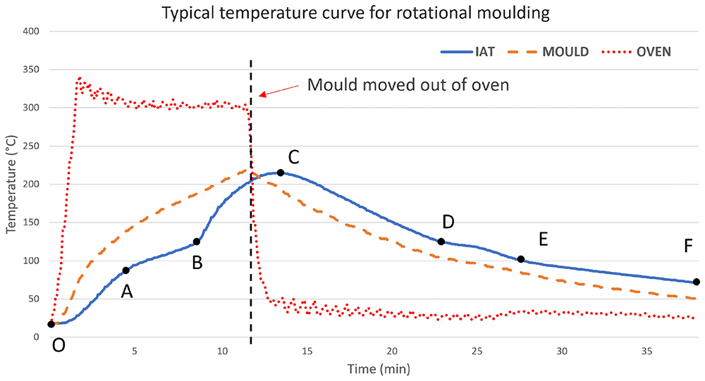
Figure 2. Typical temperature curve for oven-based rotational moulding process (laboratory records).
Apart from the heat conduction and distribution on the mould, another key factor in controlling the variance of wall thickness is the movement of the mould to distribute plastic powder within it8,9. Two distinct types of motion are employed, namely bi-axial rotation and rock-and-roll, as depicted in Figure 3. Various rotational moulding machines have been designed to accommodate specific types of motion. For instance, the Rock-and-Roll Machine, which operates under open fire impingement, is tailored for rock-and-roll motion with low cost and high efficiency but lacks process control. On the other hand, the Clamshell Machine, Shuttle Machine, and Carousel Machine are all designed to facilitate bi-axial motion with the intention of saving floor space, expanding moulding capacity and obtaining parallel operation10.
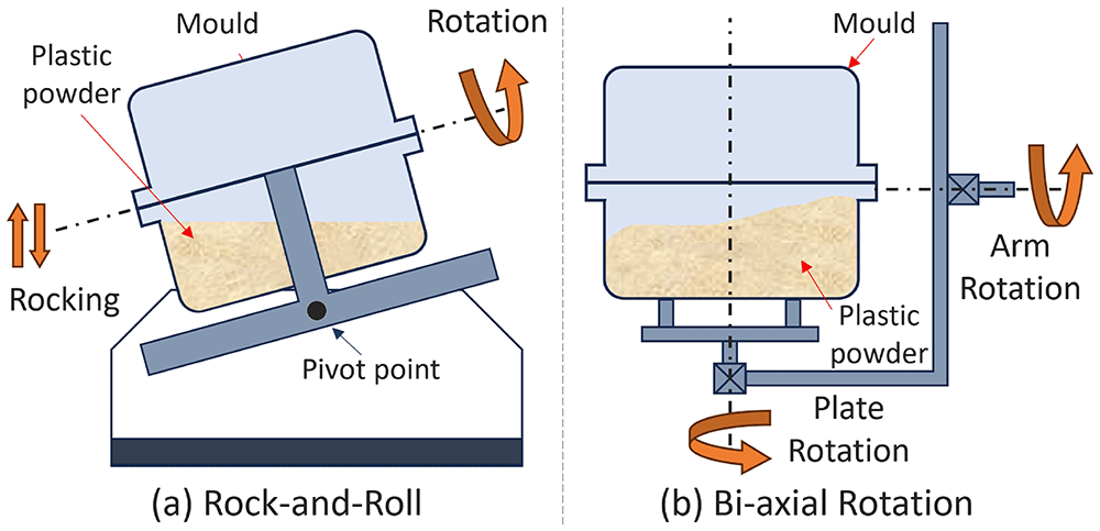
Figure 3. Two types of motion for conventional rotational moulding.
In the early years, rotational moulding was mostly based on trial and error, and the inheritance of experience. The main control variables are the temperature and oven time, as well as the limited variation in rotational speed, which leads to the simplicity of this process11,12. Due to the mould being located within an oven and its bi-axial rotation, limited measuring techniques and equipment could be used for collecting cost-effective process data13. Hence, further improvement by manipulating the key parameters was not realistic at the time. Despite rotational moulding being a relatively slow process with numerous quality specifications for the product, it still requires full-time attention from experienced operators to supervise and control the process14. The process is inherently inflexible, characterised by an excessively long cycle time. This not only impedes further development but also relegates it to being perceived as a low-tech method4.
The latest developments in computer control, mould design and motion platforms created a new vision for rotational moulding to embrace automation and intelligent technology. A simulation tool, RotoSim, which was developed at Queen’s University Belfast, has been used to aid the analysis of the moulding process since 199115,16. A recent study demonstrates the potential of using simulation to predict the shrinkage and warpage of rotational moulded parts17. Persico first developed an automated rotational moulding machine in 2002, and a compact and more capable design named SMART was launched in 201118. It uses an electric-heated mould and offers an automatic coupling docking system for quick mould change19. Both research and industrial applications in rotational moulding are gradually catching up.
Belgium company Automation & Manufacturing Service (AMS) took a step beyond the traditional machine design and integrated an electric-heated mould onto an industrial robot arm, announcing the robotic rotational moulding system (RRM, Robomould)20, shown in Figure 4. This innovation uses the robot arm to provide the rotational motion. Compared to traditional machinery, it has a distinguishable high-level flexibility in mould motion control. This system can be easily integrated with existing automation solutions with the quick-release mould changing system developed by AMS. It is also more energy efficient compared to traditional machines. McCourt et al. proved that Robomould can save 22% heating time and approximately 15 times less heating energy for the moulding of a similar part over the convection oven21.
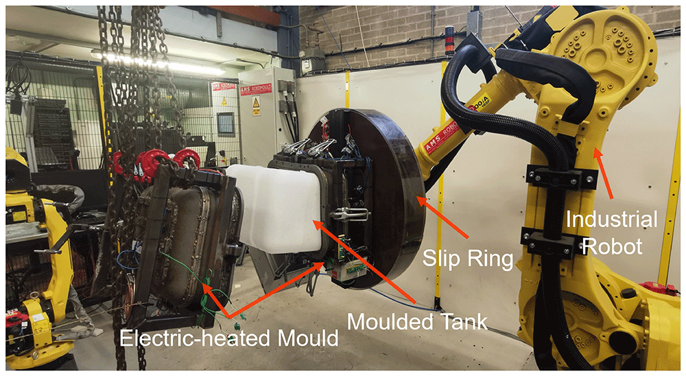
Figure 4. Robotic rotational moulding machine (Robomould).
The innovation of direct heating removes the constraint of a hot oven, enabling modern techniques for process control. However, despite this advantage, the theoretical understanding and modelling of the process have not yet been realised. As for mould motion control and the related product properties, a number of studies had been carried out since the early work of Crawford and Throne in 2002. For example, Adams et al.22 found that powder heating time and wall thickness uniformity could be affected by varying the rotational speed by using uniaxial motion and the Discrete Element Method (DEM) simulation. Głogowska et al. concluded that mould speed and the 2-axis speed ratio were capable of influencing product strength and process energy consumption23.
Mallon described 4 phases for implementing robot-based automation for injection moulding, including Pick-and-place, Value-Added Production, Cell Manufacturing and Flexible Manufacturing System24. The nature of RRM allows the system to easily achieve 4 phases by integrating multiple RRM machines with auxiliary robots and quick-release moulds25. The substantial potential of RRM lies in its ability to attain enhanced control and flexibility in the moulding process, attributed to the freedom in manipulating the mould motion beyond the constraints of traditional two-axis movement.
Ongoing tests are being conducted to assess the full capacity of this new system26. This work focused on investigating how motion parameters on RRM affect the variance of product wall thickness. Being the initial exploration of the motion control on RRM, the decision was made to focus on examining a fundamental 'rock-and-roll' motion. While the aforementioned software can simulate the conventional rotational moulding process, it lacks the capability to simulate RRM. Therefore, A motion-based finite element analysis model was created in MATLAB to study the wall thickness by simulating the distribution of powder.
Aims and objectives
This study aimed to compare the thickness distribution of moulded parts produced through RRM using both experimental and simulated methods. The objectives are as follows:
1. Explore the impact of control parameters on the wall thickness distribution of RRM products.
2. Establish a simulation model for efficiently predicting the variability in wall thickness for RRM products.
3. Validate the modelling effectiveness by comparing simulation results with experimental distributions.
Description of the RRM system
The RRM presented in this paper is based on a Fanuc R2000iA-165F with a load capacity of 165 KG. The maximum load is extendable to a maximum load of 2.3 tons with a robot system upgrade. The slip ring, depicted in Figure 3, plays a pivotal role in transmitting electric power for the heating process and maintaining air pressure or vacuum as required for pressurised moulding. The robot, programmable as a standard industrial robot, collaborates with the AMS control cabin to execute movements such as loading, cooling, demoulding, and the moulding process. Cooling is achieved by employing four air ventilation fans, each with an air moving capacity of 65 m3/min. The individual control of each fan allows for the customisation of cooling rates based on specific requirements.
The mould for this study was designed for a rectangular fuel tank with dimensions of 500 × 350 × 350 mm. Twelve tubular electric heating elements, each with a power of 1675 W, are evenly positioned on the outer surface of the mould, creating six distinct heating zones that can be independently controlled. The cumulative heating power applied to the mould amounts to 20.1 KW. K-type thermocouples are installed to monitor both the internal air temperature and the zonal temperature of the mould, facilitating precise control of the heating throughout the moulding process.
Despite six free-axis movements available on the robot arm, specifically J1 to J6, shown in Figure 3, the ‘rock-and-roll’ motion selected for RRM experiments is executed through the rotation of J5 and J6. It involves three parameters that directly describe the motion of the mould: robot feeding rate f, rocking angle θ, and the number of rotations per rocking movement r. f is the percentage of the robot's overall feeding rate or moving speed, ranging from 0% to 100%. θ ranges from 0° to 90°, denoting the rocking angle of the 5th axis of the robot arm, which moves the mould up and down. The number r can be set from 1 to 9, representing the mould rotation on the 6th axis of the robot arm and running 2 × r times when it rocks from +θ to −θ, as shown in Figure 5.
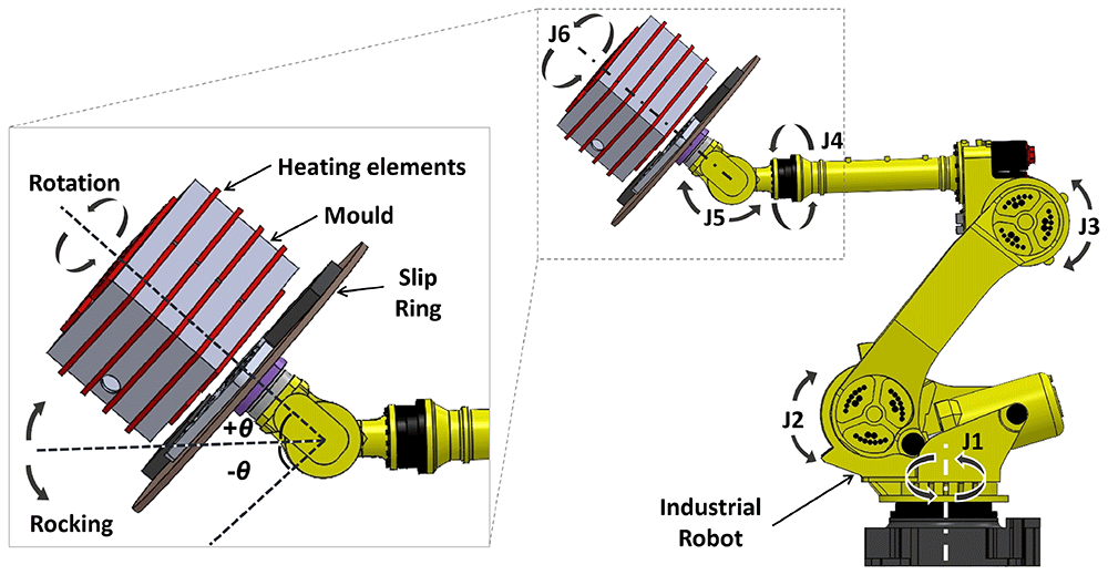
Figure 5. Definition of mould motion on the robot arm.
Design of Experiments
As described earlier in Figure 2, there is a small window for the powder to adhere to the inner mould surface from Point A to Point B. The sticky power or the melt stays in place due to the high viscosity of the polymer. The sticky powder or melt is retained in place due to the high viscosity of the polymer. Therefore, the Design of Experiments (DoE) aims to establish the relationship between processing parameters and the variability of powder deposition on the inner mould surface, ultimately influencing the variation in wall thickness for the final part.
A full-factorial design was chosen to test the effect of the 3 motion parameters on the variation of moulding wall thickness, shown in Table 1. A centre point was added to verify the linearity of the regression model. It should be noted that f < 30%, θ < 45° and r = 1n were excluded from the experiment. Initial trials showed that parameters in this range were unlikely to form an intact part. Hollow defects and partially thin-filmed walls were observed in these cases.
Table 1. Full-factorial design on robot feeding rate, rocking angle and number of rotations.
| StdOrder | RunOrder | Feed f
[%] | Angle θ
[°] | Rotation r
[n]* |
|---|
| 9 | 1 | 55 | 63 | 5 |
| 6 | 2 | 80 | 45 | 8 |
| 1 | 3 | 30 | 45 | 2 |
| 4 | 4 | 80 | 80 | 2 |
| 2 | 5 | 80 | 45 | 2 |
| 3 | 6 | 30 | 80 | 2 |
| 5 | 7 | 30 | 45 | 8 |
| 8 | 8 | 80 | 80 | 8 |
| 7 | 9 | 30 | 80 | 8 |
A further comparison group was set to determine if the amount of plastic powder would affect the variance of the thickness of the wall, as shown in Table 2.
Table 2. Extra tests for comparing the effect of the amount of power on the thickness distribution.
| Extra Test | Feed f
[%] | Angle θ
[°] | Rotation r
[n] | Reference |
|---|
| T1 | 80 | 80 | 2 | R4 |
| T2 | 80 | 45 | 2 | R5 |
| T3 | 80 | 80 | 8 | R8 |
| T4 | 80 | 45 | 8 | R2 |
Material and testing process
The experiment was performed on DOWLEX NG 2343 UE PE powder, a typical rotational moulding grade plastic material. The supplier data sheet shows a melt flow index (190 °C / 2.16 kg) of 3.8 g / 10 min (SI, ISO1133). A dry flow test was carried out to acquire the flowability and bulk density of the PE powder in the laboratory, guided by the standard from the Association of Rotational Moulders27. The results show a flow rate of 27.3 seconds and a bulk density of 358.4 kg/m3.
The moulding process followed the typical filling–heating–cooling–demoulding cycle. For the full-factorial design, each filling shot was standardised at 2.5 kg, while the additional test utilised a 4 kg filling shot. The heating ceased when the internal air temperature (IAT) reached 150 °C. Upon transitioning to the cooling stage, the IAT continued to rise, reaching the peak internal air temperature (PIAT) at approximately 200 °C, driven by the residual thermal energy in the mould. Demolding was carried out at an IAT of 90 °C following the cooling.
The demoulded part was marked by a template for the measuring points (Figure 6) and then measured by an ultrasonic thickness gauge with a measuring accuracy of ±0.05 mm. There were 16 measuring points on each face and 96 points in total for one part.
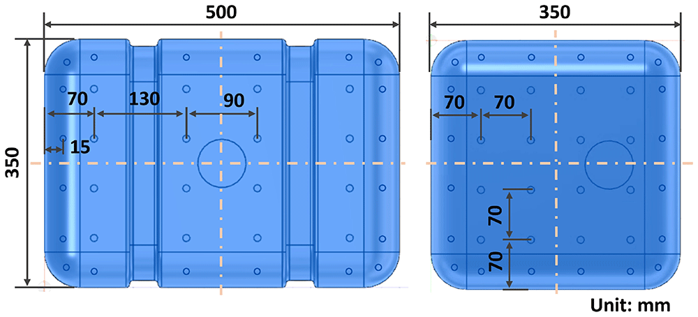
Figure 6. Measuring points on the fuel tank model.
Simulation
RotoSim, previously the sole commercially available simulation software for rotational moulding, is constrained to oven-based conventional machines in terms of its simulation objects. The fundamental assumption of RotoSim involves utilising the powder contact time on the mould surface to initiate the distribution for subsequent heat transfer and melting, eventually obtaining the thickness variation28. Given the static nature of the melt during moulding, relying solely on powder-mould contact time serves as a viable indicator for thickness distribution.
The initial attempts to use DEM simulation for obtaining the contact time distribution along the mould surface faced a significant challenge in terms of computing time. For instance, a 10-second simulation for the fuel tank mould, involving 20,000 particles, required two weeks of running time on a workstation with Xeon(R) w3-2435, 16-core CPU. In a practical scenario where 100 g of plastic powder contains millions of particles, the demand for substantial computational power renders this approach economically impractical. While reserving options like adopting high-performance computing or using fewer particles to represent the entire powder bed for exploring powder movement by DEM, a simplified model was created. This model assumes the powder bed as a deformable volume, gravitationally fitting inside the mould with a flat top surface, allowing for a swift process simulation based on the volume-mould contact.
The simulation was scripted in the software package MATLAB R2022b. It gives a quick indication of the layer thickness distribution of a formed product based on a pre-defined powder volume and robot motion. The CAD geometry of the inner surface of the mould (Figure 7) was used as input for the simulation model with a predefined position and orientation of the slip ring. The geometry was meshed to provide nodes and volume elements. The model mesh moves along the rock-and-roll robot trajectory during the simulation. Thereby, the orientation of the mould is obtained for each predefined sampling time for the whole motion trajectory. Another input for the simulation is the volume of powder. Since the position of the mould is known for the entire robot trajectory, it is possible to determine where the powder is at each time frame based on gravity.
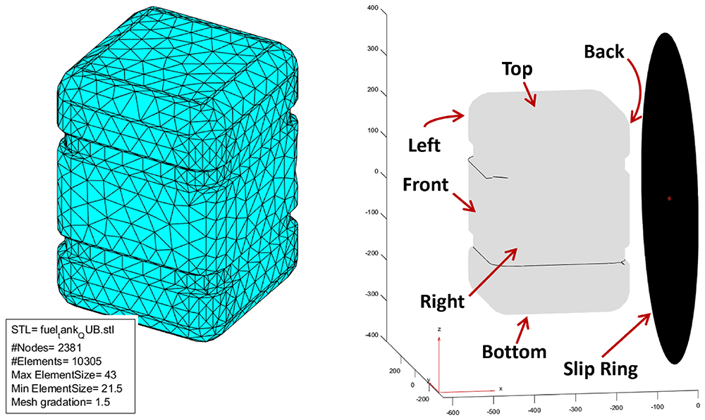
Figure 7. Fuel tank mesh geometry and orientation in MATLAB.
Following the imposed movement concluded in the simulation, a distribution plot of the powder contact time was generated on the meshed geometry. This was achieved by accumulating the active nodes that came into contact with the powder in each motion frame for the entire simulated cycle. Notably, the robot feeding rate or moulding rotation speed is not incorporated into the model, with active nodes solely relying on mould position and powder filling level. The simulation gives an indication of the layer thickness distribution of the product, based on the powder contact time as a result of the CAD geometry, the motion of the robot arm, and the volume of powder, sequentially.
To examine the uniformity of the wall thickness, the standard deviation of the contact time (STDtime) was calculated as an indicator of the thickness distribution. A lower STDtime suggests a smaller dispersion of the simulation results, which stands for a more uniform thickness distribution than a higher STDtime. The same reasoning was applied to analyse the experiment results.
Results
All the measurement data were analysed in Minitab 2020. An overview of the interval plot, shown thickness distribution of each result in Figure 8, indicates that there are significant differences among responses from different motion parameters, given that not all the confidence intervals overlap with others. In other words, there are distinguishable thickness distributions among the experimental runs from a statistical aspect. Consequently, the standard deviation of the measured thickness (STDthickness) for each mould was calculated and used as the response for factorial analysis.
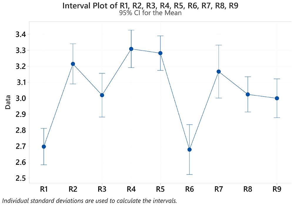
Figure 8. Interval plot of the thickness for each tank.
A Pareto chart was used to check the main effects among 3 processing parameters and their interactions. When accounting for all interaction effects, none of the factors exhibited significant effects on the deviation of wall thickness. However, the interactions of Feed × Angle × Rotation, Feed × Angle, and Feed × Rotation displayed comparatively smaller effects. Therefore, these interactions were excluded when creating a valid regression model29.
When the minor effects were removed, the normal plot of standardised effects and main effects plots in Figure 9 shows that the robot feeding rate and the interaction between rocking angle and rotation stand out. The normal probability plot reveals a well-fitted line, indicating a normal distribution of the STDthickness from the experiments. A regression equation was developed in Equation 1:
with an adjusted R-squared of 80.05 %. It highlights a strong correlation between the effects and factors, meaning the current regression explains 80.05 % of the total effects observed in the response.
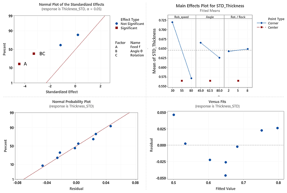
Figure 9. Effects and residual plots for the STDthickness.
However, the residual plot forms a slightly U-shaped pattern, indicating a non-linear relationship between the residual error and the regressed line. The P value for ‘Linear’ is 0.071, which is larger than 0.05, suggesting that linearity does not exist. The main effects plot confirms this by showing that the effects of the middle point are all displaced from the effect trends.
Upon direct comparison of the effects of altering each processing parameter in Figure 10, it is evident that the variation in robot feeding rate exerts the most significant impact on wall thickness change. A reduced feeding rate from 80% to 30% corresponds to a more pronounced variation in wall thickness, with a change of 0.193 in the STDthickness. Following this, the rocking angle variation shows notable influence, with a larger rocking angle of 80° compared to 45°, resulting in a smoother plot with the reduction of the STDthickness from 0.623 to 0.547. The rotations per rock, on the other hand, exhibit minimal effect on the overall shift in wall thickness, with a change in STDthickness of 0.035 from 2 rotations to 8 rotations. These observations align well with the main effect plot in Figure 9.
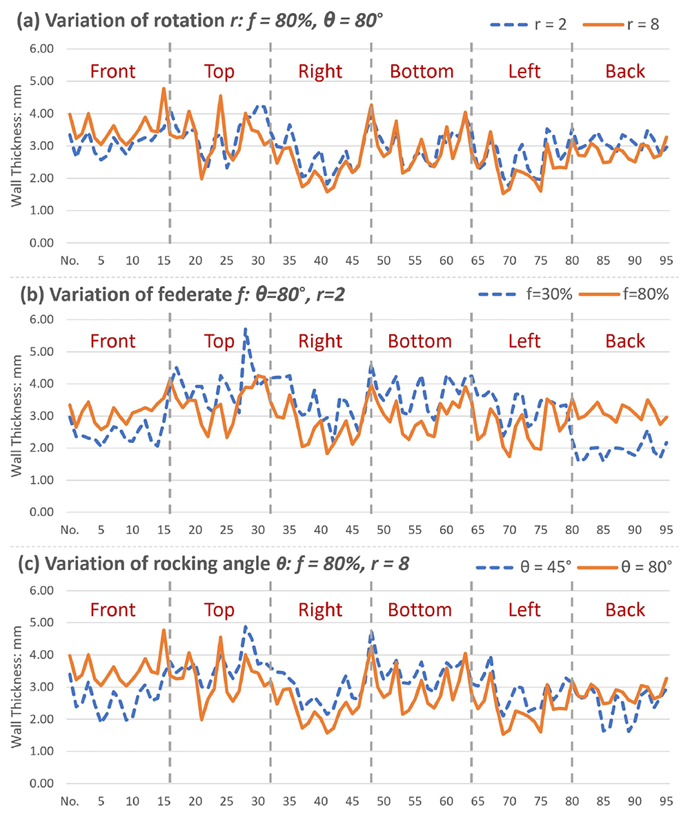
Figure 10. Effects of changing three parameters individually.
The line plots in Figure 11 illustrate the thickness distribution for 2.5 kg and 4 kg shot weight moulding using four sets of experimental parameters. Despite thicker mouldings, the 4 kg distributions closely resemble the 2.5 kg lines in all four cases, suggesting that shot weight does not significantly impact the thickness distribution pattern in the experimental groups. This observation is further supported by the correlations presented in Table 3, where the high correlation coefficients, ranging from 0.83 to 0.93, indicate a strong positive linear relationship between the thickness distributions at the two different shot weights.
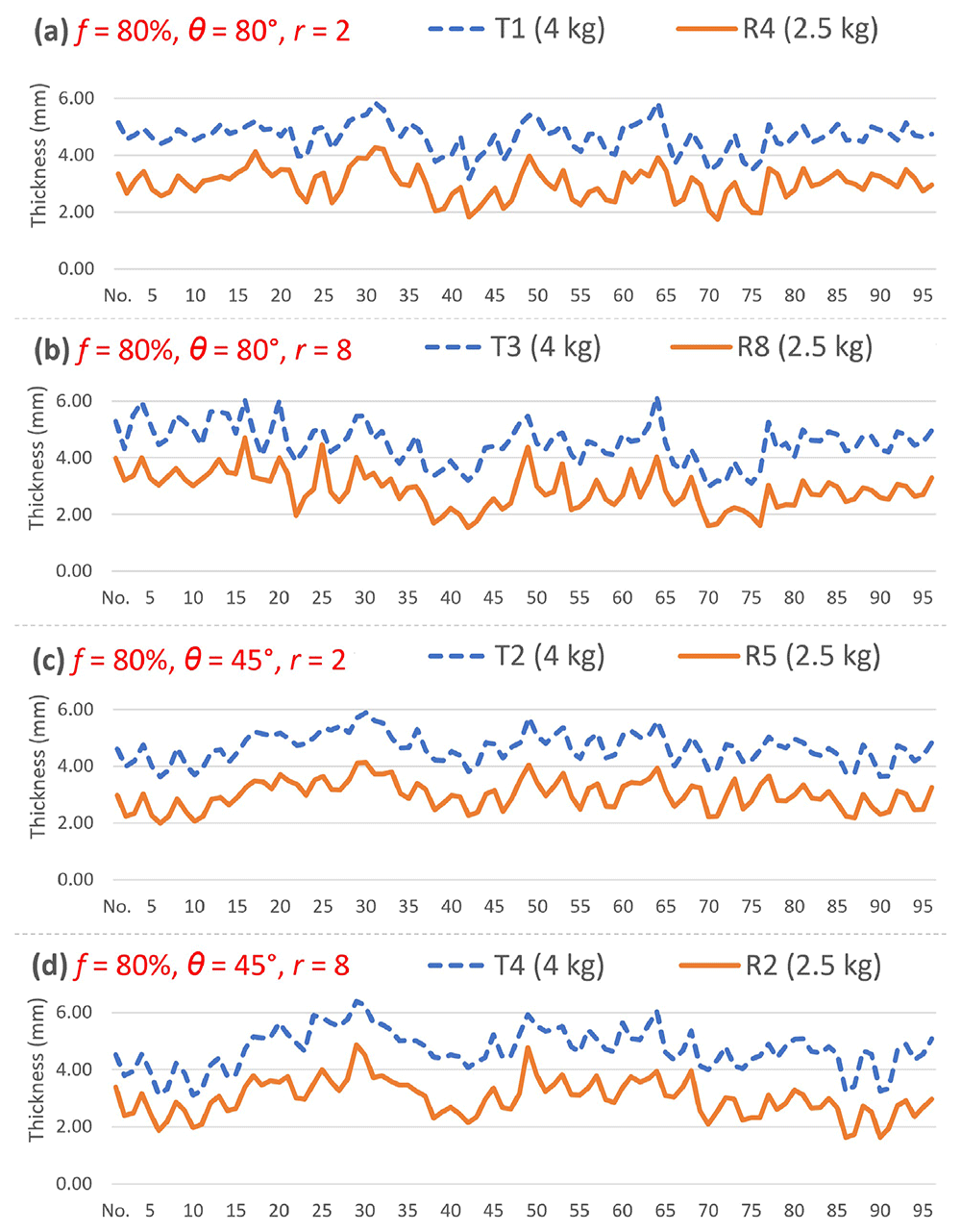
Figure 11. Thickness distribution comparison for different filling shot weights.
Table 3. The correlation of the thickness distribution between 2.5 kg and 4 kg shot weight.
| Extra Test | Feed f
[%] | Angle θ
[°] | Rotation r
[n] | Reference | Correlation
2.5 – 4 kg |
|---|
| T1 | 80 | 80 | 2 | R4 | 0.91 |
| T2 | 80 | 45 | 2 | R5 | 0.93 |
| T3 | 80 | 80 | 8 | R8 | 0.83 |
| T4 | 80 | 45 | 8 | R2 | 0.91 |
The simulation model does not incorporate robot speed as an input for estimating the distribution. Therefore, the experimental results with high and low feeding rates were compared with the simulation, keeping the rocking angle and the number of rotations constant. In Figure 12, the left side shows the simulated distribution, while the right side presents thickness measurements from the experiment, with one representative sample out of nine simulation results. The 30% feed case showed a better match between the simulated contact time distribution and the experimental thickness distribution than the 80% feed case.
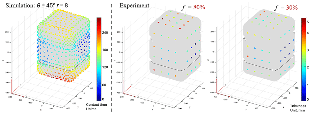
Figure 12. Comparison between the simulation results and experimental results.
To assess the model's predictive capability, a comparative analysis was performed by calculating the normalised Standard Deviation of Contact Time (STD’time) from the simulation and comparing it with the normalised Standard Deviation of Thickness (STD’thickness) from experimental measurements. Both datasets were normalised using their respective average values, as shown in Table 4, where a red–yellow–green colour scale is applied to indicate the values. The correlation analysis revealed varying levels of alignment between the two Feed levels: a correlation coefficient of 0.58 for the 30% feed group and 0.29 for the 80% feed group.
Table 4. Comparison of normalised STD’thickness from experiment and STD’time from simulation.
| STD_ORDER | Feed
[%] | STD’
thickness | STD’
time |
|---|
| 1 | 30% | 1.07 | 1.21 |
| 3 | 1.22 | 1.21 |
| 5 | 1.29 | 0.84 |
| 7 | 0.95 | 0.89 |
| 9 | 55% | 0.89 | 0.71 |
| 2 | 80% | 0.84 | 1.21 |
| 4 | 0.91 | 1.21 |
| 6 | 0.98 | 0.84 |
| 8 | 0.86 | 0.89 |
To visualise the simulation prediction, a series of simulations was carried out with rocking angles ranging from 25° to 85° with 5° intervals, and the number of rotations per rocking movement from 1 to 8. The STDtime obtained from the simulation is shown in Figure 13. Firstly, this suggests that the STDtime initially reduces with the increase in rocking angle and then climbs again after 60°. Secondly, STDtime declines gradually with the growth of the number of rotations, but the gradient reduces at larger numbers and reverses the effect after 7 rotations per rock. The smallest STDtime is observed at θ = 60° and r = 7 among these simulations.
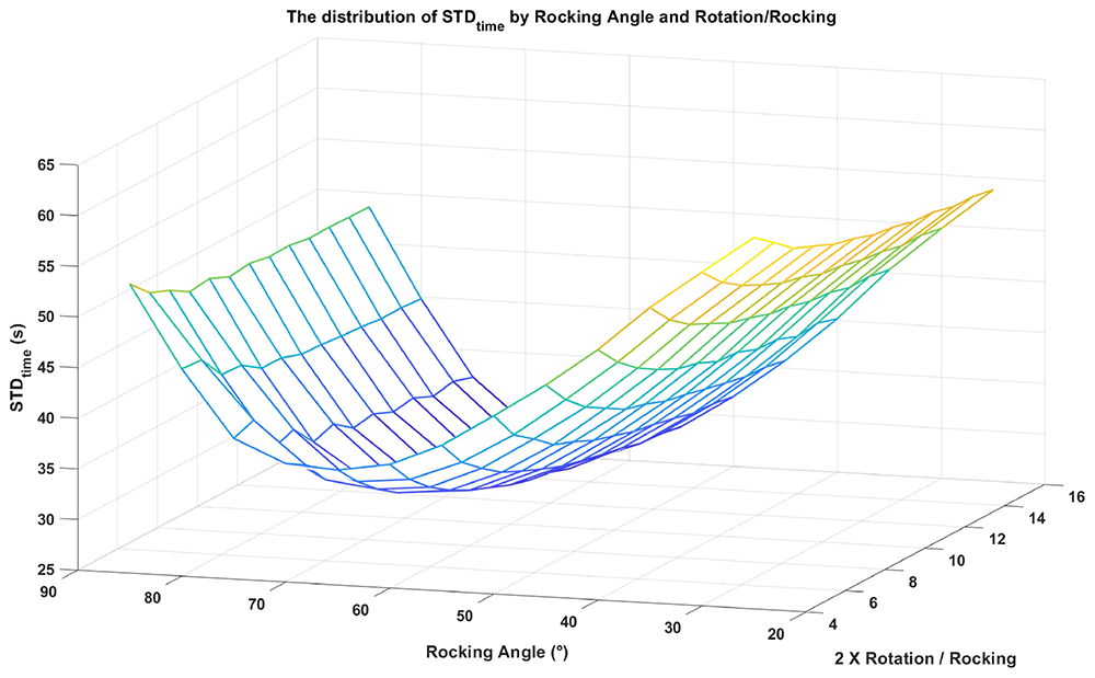
Figure 13. Plot of the STDtime based on 174 moulding simulations.
Discussion
The full-factorial design is based on the assumption of linear response with the factors. The P-value for linearity, the residual plot and the central point test contradict this assumption. The simulation results also propose the presence of curvature in the effects. Nevertheless, some useful information can be extracted from the regression model.
According to the regression model, the key factors influencing the wall thickness distribution are the robot speed and the interaction between rocking angle and mould rotation. Existing literature highlights the significant influence of mould rotation speed and the two-axis ratio on powder bed movement and, consequently, on thickness distribution4,7. Given the differences between a conventional machine and the RRM, an important question arises: do these two factors exert the same effect in the RRM context? In conventional rock-and-roll machines, the rocking pivot is positioned at the mould’s centre or centre of gravity, resulting in a side-to-side rocking motion. In contrast, the RRM pivot lies at the mould’s side, creating an up-and-down rocking motion. While it is clear that robot feeding rate governs rotation speed and strongly affects distribution, it remains uncertain whether the speed ratio has a comparable effect in RRM.
In the current motion control setting of the RRM, the mould finishes the rocking at θ degrees while rotating r times with full 360° rotations. Assuming a constant C converting robot feeding rate f into mould rotation speed ω1 = Cf, then the time for complete r rotations, as well as rocking degrees of θ, is t = r / ω1. The rocking speed is ω2 = θ / t. Using the speed ratio equation Equation 2:
the speed ratio for the RRM system can be calculated in Equation 3:
The equation shows that the RRM speed ratio is only dependent on the ratio of rocking angle θ versus mould rotations r. The interaction between θ and r happens to be the second significant effect of the regression model of the full-factorial design. The results support the idea that the thickness distribution of the RRM is determined by the mould rotation speed (defined by f) and two-axis speed ratio (defined by θ/r). Despite the rocking pivot point being far away from the mould centre of gravity, RRM with a different structure and rocking motion, inherits the essence of motion control from the traditional machine.
It is plausible that results from the 4 kg comparison group exhibit the same distribution pattern as their 2.5 kg counterparts. This suggests that the control parameters do not need to be altered for either thicker or thinner mouldings. Although the larger powder pool in the 4 kg experiment leads to a broader contact surface, the movement of the powder pool during moulding remains consistent. It is conceivable that the smaller sweeping area with 2.5 kg could yield a similar powder deposition on the inner surface, compared to the larger sweeping area with 4 kg, given sufficient overlapping in each sweep is achieved during the moulding.
Owing to the absence of defining dynamic properties for the powder flow, the simulation model does not fully represent the real powder flow circumstances. While using particle-wall contact time is an essential simplification in simulations, it might introduce errors in representing the wall thickness buildup. Additionally, the model's core assumption of a constant flat powder surface neglects the dynamic formation of the powder bed with its dynamic angle of repose, potentially influencing the actual powder contact area within the mould.
A validation moulding was conducted with the parameters from the best predicted STDtime. The robot feeding rate was set as 80% to achieve better distribution. Figure 14 exhibits a marked consistency in distribution between the simulation and experiment, with some disparities observed at the bottom face. The right and left faces display similar patterns but exhibit larger displacements from the experimental distribution compared to other faces.
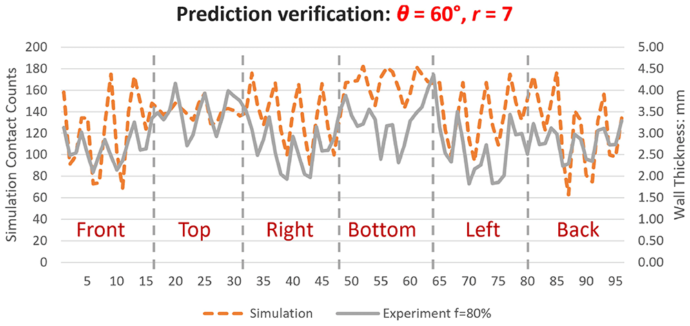
Figure 14. Validation of the best prediction obtained from the simulation.
To further validate the simulation model and DoE, the parameter sets with the worst prediction from simulation and the one with the best prediction from linear regression were also moulded for comparison. Comprehensive details, including STDthickness calculated from measured thickness, are presented in Table 5. Moulding with the best-predicted parameters by simulation has an STDthickness of 0.599, slightly larger than the smallest STDthickness of 0.536 among the experimental results. Conversely, moulding by the worst prediction has an STDthickness of 0.814, only 0.09 smaller than the worst experimental results. The moulding with the best-predicted parameters by linear regression has a STDthickness of 0.540, almost equal to the smallest one in the DoE. These results demonstrate a strong agreement between the simulation and experiment. Despite the aforementioned curvature observed from the analysis of DoE, the validation of the best prediction by regression still indicates a favourable trend in utilising the correct parameters to achieve a more uniform distribution of wall thickness.
Table 5. STDthickness results for the validation of DoE and simulation.
| StdOrder | RunOrder | Feed f
[%] | Angle θ
[°] | Rotation r
[n] | STDthickness | Note |
|---|
| 1 | R3 | 30 | 45 | 2 | 0.679 | DoE |
| 2 | R5 | 80 | 45 | 2 | 0.536 | DoE |
| 3 | R6 | 30 | 80 | 2 | 0.774 | DoE |
| 4 | R4 | 80 | 80 | 2 | 0.581 | DoE |
| 5 | R7 | 30 | 45 | 8 | 0.823 | DoE |
| 6 | R2 | 80 | 45 | 8 | 0.623 | DoE |
| 7 | R9 | 30 | 80 | 8 | 0.602 | DoE |
| 8 | R8 | 80 | 80 | 8 | 0.547 | DoE |
| 9 | R1 | 55 | 63 | 5 | 0.565 | DoE |
| V1 | / | 80 | 60 | 7 | 0.599 | Best Prediction / Simulation |
| V2 | / | 80 | 25 | 2 | 0.814 | Worst Prediction / Simulation |
| V3 | / | 100 | 85 | 9 | 0.540 | Best Prediction / DoE Regression |
Up to this point, the simulation model has proven its utility in providing valuable distribution information for an RRM process. However, some corrections are still required, particularly for better fitting the left, right, and bottom faces of the tank. Implementing an additional response surface design to identify non-linear responses will aid in discovering the true relationship between the effects of thickness distribution and motion parameters.
It is noteworthy that the completion of a single simulation on a standard PC typically takes less than one minute for this motion-based simulation. Although the accuracy is expected to be improved, it outweighs the simulation running time of RotoSim, which requires 15 to 20 minutes for one run. This is particularly advantageous when considering the significantly longer running time associated with DEM simulation. This model can efficiently offer a rapid distribution profile for specific moulding setups, requiring minimal computing resources.
Conclusions
The findings of this investigation have contributed to bridging certain gaps in the comprehension of this innovative robotic-based rotational moulding machine. It can be concluded that:
1. The thickness distribution of parts moulded by RRM using rock-and-roll motion is mainly determined by the same two factors as in the traditional machines: (a) the mould rotation speed described by robot feeding rate f, and (b) the two-axis speed ratio as described by the ratio of the number of rotations per rocking r versus the rocking angle θ.
2. A higher robot feeding rate is preferred for a better overall thickness distribution. However, a better ratio for r / θ may exist in the hidden curved response.
3. The influence of varying shot weights on the wall thickness distribution pattern is negligible within the experimental groups.
4. A highly simplified motion-based simulation model can provide fast prediction of the powder distribution trend, which can be applied to indicate the thickness distribution on a known product geometry with prescribed motion.
Future works
Considering the non-linear response was detected from the full-factorial design, a surface response design is planned to further study the relationship between the thickness distribution and Robomould motion parameters. In addition, corner thickness was not measured in this study due to the difficulty of measuring curved surfaces with the current ultrasonic gauge. Since powder tends to accumulate at corners during the moulding process, corner measurements will be included in future work.
Regarding the simulation, the current model is a strong simplification of reality with no dynamic properties of the powder included. The powder lies and moves in the mould entirely under the gravity applied. To improve the simulation, three important changes are planned. Firstly, adding a certain inclination angle (the dynamic angle) of the powder bed, which depends on the rotation speed, temperature and the specific powder characteristics. Secondly, adding a powder reduction mechanism during the moulding process, where powder dissipates and sticks to the inner surface of the mould. Thirdly, considering powder property changes with the temperature in the tacky and melting stage. After implementing these extensions, it is expected that the accuracy of the simulation results will increase and thus better match reality.
Ethics and consent
Ethical approval and consent were not required.
Data availability
Underlying data
Open Research Repository (Data Repository at Queen's University Belfast ): Dataset for 'Study of thickness distribution on a robotic rotational moulding system by experiment and simulation'. DOI: https://doi.org/10.17034/30230857.v130.
The project contains the following underlying data:
Definition of faces on the fuel tank.jpg (Defined the name and location of six faces of the fuel tank relative to the robotic rotational moulding system.)
Measuring points on the fuel tank model.jpg (Defined the measuring point locations on the fuel tank.)
Design of Experiment.jpg (Define the experiment design.)
Measurement data for Study of thickness distribution on a robotic rotational moulding system_v2.csv (Recording of wall thickness measuring results from all the moulded fuel tanks.)
STDtime of simulated surface contact time for various motion settings.csv (Records of simulated polymer contact time STDtime for plotting the Figure 13.)
Data are available under the terms of the Creative Commons Attribution 4.0 International license (CC-BY 4.0).
Acknowledgements
The authors wish to thank AMS, Belgium, for their support for this work, and in particular for providing the RRM machine and mould on which the work was carried out. J. Vanherck gratefully acknowledges the financial support provided by the Flanders Innovation & Entrepreneurship Agency. The assistance of the Internal Funds KU Leuven is also highly appreciated.
Faculty Opinions recommendedReferences
- 1.
Wilson M:
Chapter 1 - Introduction. In: Implementation of robot systems. Elsevier Inc, 2015; 1–18.
- 2.
Hyland I:
Robots used on plastic injection moulding machines.
Ind Rob.
2001; 28(2): 104–111. Publisher Full Text
- 3.
Crawford RJ:
Reducing cycle times in rotational moulding - a challenge. Annual Technical Conference - ANTEC, Conference Proceedings. 1998; 1. : 1108–1111.
- 4.
Nugent P:
15 - Rotational molding. In: Kutz (Ed.), Applied plastics engineering handbook (Second Edition), Plastics Design Library. William Andrew Publishing, 2017; 321–343. Publisher Full Text
- 5.
Crawford RJ, Throne JL:
1 - INTRODUCTION TO ROTATIONAL MOLDING. In: R.J. Crawford, J.L.Throne (Eds.), Rotational molding technology, plastics design library, William Andrew Publishing, Norwich, NY, 2002; 1–18. Publisher Full Text
- 6.
Crawford RJ, Nugent PJ:
A new process control system for rotational moulding.
Plastics, Rubber and Composites Processing and Applications.
1992; 17: 23–31. Reference Source
- 7.
Beall GL:
Rotational molding: design, materials, tooling, and processing. Munich: Hanser, 1998. Reference Source
- 8.
Crawford RJ, Throne JL:
6 - PROCESSING. In: R.J. Crawford, J.L.Throne (Eds.), Rotational Molding Technology, Plastics Design Library. William Andrew Publishing, Norwich, NY, 2002; 201–306. Publisher Full Text
- 9.
Adams J, Jin Y, Barnes D, et al.:
Simulation of the rotational moulding process using discrete element methods. 34th International Manufacturing Conference. 2017; 136. : 23–42.
- 10.
Crawford RJ, Throne JL:
4 - ROTATIONAL MOLDING MACHINES. In: R.J. Crawford, J.L.Throne (Eds.), Rotational Molding Technology, Plastics Design Library. William Andrew Publishing, Norwich, NY, 2002; 111–148. Publisher Full Text
- 11.
Cramez MC, Oliveira MJ, Crawford RJ:
Optimisation of rotational moulding of polyethylene by predicting antioxidant consumption.
Polym Degrad Stab.
2002; 75(2): 321–327. Publisher Full Text
- 12.
Crawford RJ, Kearns MP:
Practical guide to Rotational Moulding. Smithers Rapra, Shrewsbury, 2012. Reference Source
- 13.
Ramkumar PL, Ramesh A, Alvenkar PP, et al.:
Prediction of heating cycle time in Rotational Moulding.
Mater Today Proc.
2015; 2(4–5): 3212–3219. Publisher Full Text
- 14.
Rodrigues M, Mendes J, Fonseca J:
Application of a web-based monitoring and control system in plastic rotational moulding machine. Proceedings of the IEEE International Conference on Industrial Technology. 2004; 2. : 819–823. Publisher Full Text
- 15.
Crawford RJ, Nugent P, Xin W:
Prediction of optimum process conditions for rotomolded products.
Int Polym Process.
1991; 6(1): 56–60. Publisher Full Text
- 16.
Nugent PJ, Crawford RJ, Xu L:
Computer prediction of cycle times during rotational molding of plastics.
Adv Polym Technol.
1992; 11: 181–191. Publisher Full Text
- 17.
Seregar J, McCourt MP, Kearns MP, et al.:
Simulation of shrinkage and warpage of rotationally moulded polymer parts.
Procedia Manuf.
2020; 47: 987–990. Publisher Full Text
- 18.
ARMO:
2018–2019 ARMO Rotational Moulding product showcase by Jennifer Gibson Hebert - issuu. 2018; (accessed July 15, 2024). Reference Source
- 19.
Persico:
Smart technology by Persico. 2021; (accessed July 15, 2024). Reference Source
- 20.
Kuijt J, Kuijt B, Harleman F, et al.:
Device for rotational molding of plastic material. U.S. Patent No. US9327431B2. 2016. Reference Source
- 21.
McCourt MP, Kearns MP, Martin PJ, et al.:
A Comparison between conventional and robotic rotational moulding machines. In: 34th International Manufacturing Conference. Ireland, 2017. Reference Source
- 22.
Adams J, Jin Y, Barnes D, et al.:
Motion control for uniaxial rotational molding.
J Appl Polym Sci.
2021; 138(8): 1–14. Publisher Full Text
- 23.
Głogowska K, Longwic F, Ludziak K:
Effect of mould speed on selected properties of moulded parts and energy consumption in rotational moulding.
Bull Pol Acad Sci Tech Sci.
2022; 70(5): 1–10. Publisher Full Text
- 24.
Mallon JM:
Advances in automation for plastics injection moulding. iSmithers Rapra Publishing, 2001. Reference Source
- 25.
AMS:
AMS 4.0 global automation. 2021; (accessed June 19, 2024). Reference Source
- 26.
Zhou H, Martin P, McCourt M:
Advanced process control in robotic rotational moulding. In: IMC37. Athlone. 2021; 135–141. Reference Source
- 27.
Association of rotational molders:
Test Method for Particle Size of Rotational Molding Powders. Association of Rotational Molders, 2015. Reference Source
- 28.
Crawford RJ, Nugent PJ:
Computer simulation of the rotational moulding process for plastics.
Plastics and Rubber Processing and Applications.
1989; 11(2): 107–124. Reference Source
- 29.
Harrell FE:
Describing, resampling, validating, and simplifying the model. In: Jr. Harrell Frank E. (Ed.), Regression Modeling Strategies. Springer International Publishing, Cham, 2015; 103–126. Publisher Full Text
- 30.
Zhou H:
Dataset for “Study of thickness distribution on a robotic rotational moulding system by experiment and simulation”. 2025. http://www.doi.org/10.17034/30230857.v1