There is extensive literature on the relationship between two or more countries that uses DSGE models. The existing literature can be divided into three main groups. The first group includes models that consider an infinite number of small open economies without the power to change the aggregate equilibrium. This is the case in the model of Gali and Monacelli (2005), who studied a monetary union with an infinite number of economies and shared monetary authority. They found that "despite this joint monetary-fiscal regime being designed in order to maximize the welfare of the union as a whole, optimal fiscal policy in each member country calls, in equilibrium, for a macroeconomic stabilization role that goes beyond the one consistent with the optimal provision of public good." This conclusion has obvious implications for the stabilization of a monetary union without strong fiscal authority. A similar result was found by Faia and Monacelli (2008), where in the same infinite economies framework, they allow each economy to have its own monetary authority. They found that "home bias in consumption is a sufficient condition for inducing the monetary policy maker of an open economy to deviate from a strategy of strict markup stabilization.” In essence, both show that a long list of conditions is necessary for fiscal and monetary authorities to implement a policy that would be optimal for the aggregate union but not necessarily for each individual entity inside it. In these cases, deviations from aggregate equilibria yield better outcomes for the individual country.
The second main group is the most extensive, consisting of models with two countries, where each country has its own currency and their central bank must decide whether to commit to a common objective. This is the case in the model of Clarida et al. (2002), where two central banks must decide whether to cooperate. They found that there are gains from cooperation, but to achieve it, central banks have to react to foreign inflation as well as to national inflation. Under Nash equilibrium, central banks only need to react to domestic inflation. Ida (2013) followed a similar approach and found that cooperation was not optimal when both economies hit the zero lower bound. Under similar conditions, Pappa (2004) conducts a welfare analysis to compare the equilibrium in three possible arrangements: a cooperative equilibrium, a non-cooperative equilibrium, and a monetary union. He finds that "the non-cooperative equilibrium may be suboptimal because of terms of trade spillover effects, while the monetary union may be suboptimal because of the sluggishness of relative prices."
To guarantee the existence of an equilibrium, the authors need each economy to have its own central bank. When both countries have their own central bank following an inflation targeting rule, but they do not have common or individual fiscal authorities powerful enough to stabilize the economy, the uniqueness of the equilibria is not guaranteed. guaranteed. Bullard and Schaling (2009) studied this problem in the environment created by Clarida et al. (2002), and described the conditions under which the uniqueness of equilibrium can be achieved. They found that if a country inside a union deviates from equilibrium, all other countries will be unable to attain equilibrium by themselves. Batini et al. (2004) took a different approach to the same problem and studied the determinacy problem using inflation-forecast-based rules instead of the common Taylor Rules used in one-country New Keynesian models. Under this methodology, first employed by Batini and Pearlman (2002), they obtain a unique stable equilibrium with a two-world economy.
The third group consists of models in which certain conditions are added to the policy rule to guarantee equilibrium. This is the case in Benigno (2004), who proposes to give a higher weight in the policy rule to the inflation of the country with a higher degree of nominal rigidity inside the monetary union. With this modification, he is able to guarantee determinacy and nearly optimal equilibrium. Another possible approach to guaranteeing equilibrium determinacy is that proposed by Ferrero (2009). In a monetary union with individual fiscal authorities, he advocates that those fiscal authorities be in charge of smoothing the impact of idiosyncratic exogenous shocks, while the monetary authority focuses on maintaining overall price stability.
Ferrero (2009) proposed the only solution for equilibrium determinacy, consistent with the European Central Bank (ECB) mandate. To guarantee the equilibria, this approach needs all individual fiscal authorities to be powerful enough to stabilize their economy on their own, as a substitute for the common fiscal authorities used in one-country models. This last case is observed in the US, where the US Treasure plays the role of a common and powerful fiscal authority. However, the EA, where such an authority does not exist, needs to assume sufficiently powerful individual authorities to stabilize each individual economy. In the recent past, the EA sovereign debt crisis showed that this assumption may be too strong to hold. During this crisis, some countries such as Greece and Portugal were unable to finance themselves in international financial markets, making it necessary for international institutions to guarantee their solvency.
The remainder of this paper is organized as follows. In Section 1 I develop a two-country New Keynesian model with a common central bank suffering a multiplicity of equilibria. From this model, I compute the welfare loss function to determine which variables drive it. Then, I use this function to build a policy rule that I estimate for the US and EA in Section 3. Finally, Section 4 concludes the paper.
1. The model
New Keynesian models are a common approach for analyzing the effect of choosing between different monetary policy rules. Using a New Keynesian model, I would be able to test different policy rules to determine which yields a lower social welfare loss. However, this approach has a problem: a two-country model with an inflation-targeting central bank like the ECB does not fulfil the Blanckard-Khan conditions, resulting in a multiplicity of equilibria. More than one equilibrium is possible, and the equilibrium reached depends on the initial conditions. As discussed earlier, the only solution proposed in the literature, consistent with EA treaties, is that of Ferrero (2009). However, for this to work, the EA needs individual authorities to be strong enough to stabilize their economies. If these authorities are not sufficiently strong, the central bank will not be able to react with its full strength to output and/or inflation deviations in the union.
The inability of individual fiscal authorities to stabilize their economy will be patent when the heterogeneity between countries starts affecting the monetary policy determination for the whole union. This heterogeneity between countries can be captured in terms of trade in the following two-country New Keynesian model.
I am developing the simplest case of a Monetary Union, in which two countries decide to share a unique currency without a political union. As a consequence of this union, the Central Bank must decide which monetary policy to implement, taking into account the interests of both countries. The two regions, home (H) and foreign (F), may differ in size but are otherwise symmetrical. In the Home country, it is assumed to live in the γ proportion of the total population, whereas in the foreign country, the remaining 1 – γ of the population lives. I assumed this population to be a continuum in the interval [0,1]. Therefore, the population in segment [0,γ] lives in the home country, and the population in segment [γ, 1] lives in the foreign country. Households in both countries also have access to Arrow-Debreu securities, which can be traded both domestically and internationally.
1.1. Home country households
I followed the lines of the model developed by Clarida et al. (2002) for a two-block world. The big difference between the two is in how the monetary policy is set. While they assume two central banks that individually set their monetary policy, I assume a common central bank that sets the monetary policy for the whole union. According to the ECB Governing Council,2 the central bank reacts to weighted average inflation. Households choose between home and foreign goods according to
where CHt and CFt are the indexes of consumption across the continuum of differentiated goods produced in countries H and F, respectively.
where Ct(h) denotes the quantity of good h ∈ [0,γ], produced in the home country consumed by each household in period t. Similarly, Ct(f) stands for the quantity of foreign produced goods f ∈ [γ, 1] consumed by the national household in period t. For convenience, I assume that the number of firms is equal to the number of households in each country.
The elasticity of substitution across the goods produced in a country is ε. I assume that there is no home bias in consumption; the elasticity of substitution between home and foreign consumption will then be the proportion of the population in the national economy (γ).
Individual firms will minimize costs yielding the following relations:
From the above assumption, we derive the aggregate price index for the goods produced in each country:
where Pt(h) is the price for the home country produced goods and Pt(f) is the price for foreign country produced goods. Similarly, PHt is the aggregate price of the home country producing consumption goods, and PFt is the aggregate price of consumption goods produced in the foreign economy.
Conditional on optimal behaviour:
The total consumption expenditure for each type of good can be written as a product of the price index multiplied by the quantity index.
The maximization of Equation (1) s.t. PHtCHt + PFtCFt ≡ Xt yields:
1.1.1 Utility maximization. The preferences of a representative household in the home country are given by the following function, which is maximized with respect to the budget constraint:
where Zt is an exogenous preference shifter. β ∈ (0,1) denotes the discount factor. Wt is the nominal wage. Bt are the nominal riskless discount bonds purchased in period t. Rt is the interest rate for the period bonds.
FOC
A first order approximation to Equation (9) yields:
where lowercase letters represent deviations from the non-inflationary steady state. Equation (11) can be seen as a competitive labor supply schedule, where the amount of labor supplied is a function of the real wage and utility of consumption. where the parameter φ is the inverse Fisher labor supply elasticity.
A first-order approximation around the zero-inflation steady state in Equation (10) yields the Euler equation for consumption:.
where πt+1 = pt+1 – pt is the inflation rate between t and t+1 in the home economy. The preference shock is assumed to follow an autoregressive process, according to Similarly, ĉt is the home consumption deviation from the steady state, and is the interest rate deviation from the steady state.
1.2. National firms
The national production of a specific variety of goods is the sum of their consumption in both countries.
where Ct(h)* stands for consumption in the foreign economy-specific variety of goods produced in the home country. represents aggregate world consumption, and represents terms of trade.
Defining Yt as:
Using Equation (13) in the above equation, we obtain an equation linking output and consumption:.
where and
1.3. Aggregate employment
The number of firms is assumed to be equal to the number of households. The home country has a continuum of firms, indexed by i ∈ [0,γ]. Each firm produces a differentiated good, but all of them use the same technology according to
where At denotes the technology level. Technology is assumed to be common to all firms operating in the home country. Aggregate employment in the home country is the sum of employment across firms.
Using the production function from Equation (17) and Equation (16), we can write
which linearised with respect to the non-inflationary SS:
where ât is the technological deviation from the steady state. It evolves according to the autoregressive process with ρa ∈ [0,1]. Up to a first-order approximation, is zero in the neighborhood of zero-inflation SS. Then,
1.4. Risk sharing
The monetary union’s interest rate must be equal for both countries. Then, using Equation (10) and its foreign economy counterpart, we can write
Combining the above with the law of one price, and considering the model around a symmetric equilibrium:
which linearised around the symmetric non-inflationary steady state:
1.5. Welfare analysis
The last step in closing the above model is to introduce a policy rule consistent with the ECB mandate. Rotemberg and Woodford’s (1999) seminal work established a second-order approximation of utility losses as the baseline criterion to find the optimal policy rule. When I apply this methodology to this model, a new variable appears in the welfare loss function: the terms of trade. This variable accounts for the trade between both economies produced by the price difference between home and foreign goods. For the model considered in this chapter, the second-order approximation of consumer welfare losses can be written as a function of steady-state consumption as
The second-order Taylor expansion for the utility function in the home country around the steady state can be written with respect to the output by using Equation (20). After some manipulation, I obtain:
where t.i.p. stands for terms independent of policy.
The efficiency in SS implies (1 – α)(Y/N) = (Nφ/C–σ). From the risk-sharing condition in Equation (22), C = C* in the SS, using Equation (15), I find Y = C. Using these conditions in Equation (25), I can write:
A second order approximation around yields 3
As shown in Woodford (2003), Using this result in the above equation and linearization of Equation (8), we can write Equation (27) as
In the same way, the equation for the foreign country will be:
Substituting Equation (28) and Equation (29) into Equation (24), we obtain
The average welfare loss per period is given by a linear combination of the variances in the output gap, inflation, and terms of trade.
In the case of a monetary union like the one considered above, I have shown that the welfare loss function is not only a function of the output and inflation gap but also of the terms of trade. If the central bank of a union like this one wants to find the best policy rule, it should consider the terms of trade, in addition to the output and inflation gaps of the union.
From a mathematical perspective, it is possible to study the optimal policy function for the monetary union from a benevolent central planar perspective. However, as in any other central planner equilibrium, it is necessary to assume that the monetary authority is able to choose the desired levels of inflation and output gap at each point in time. In practice, without the existence of a central planner, central banks cannot set either variable directly. The most common approach in the literature to address this problem is to adopt an interest-rate rule that guarantees the desired outcome. The most common interest rules in monetary policy analysis are those derived from Taylor (1999), who relate interest rates to output and inflation gaps.
A regular Taylor rule weighted by the size of each economy in the monetary union, like the one established by the ECB Governing Council, would look like
With this rule, the monetary authority reacts to union output and inflation gaps with the same structure as that currently used by the ECB. However, this rule leaves aside a variable that appears in the welfare loss function of the union: the terms of trade (st).
2. Estimation of the terms of trade
The next step in this analysis is to find a proxy variable for terms of trade. In Model I, terms of trade are defined ŝt ≡ pFt – pHt. Terms of trade are the difference between the prices in one country and the other in a two-country monetary union. In the real world, we do not have two-country unions, but multilateral unions. The EA comprises 19 countries, and the US has 50 states in addition to the District of Columbia. Consequently, I have two options: to create two countries with an aggregate of countries/states, or to find a way to compute the terms of trade for the whole union. The first option has a big problem: the countries/states are not easy to divide into two groups because of the heterogeneity between countries. In addition, some effects could be masked by aggregation, as happens when I aggregate for the entire union. This makes the second alternative the most representative of what is happening in a union.
To estimate the terms of trade from individual states/countries, I need to use a statistic compiling all this information. From the definition of the terms of trade, the first option would be to use the average difference between each country’s prices and union prices:
This statistic estimates the average price deviation of each country from the union. However, all countries/states have the same weight in the statistics. This is unreliable because some countries/states are much larger than others in terms of both GDP and population. The weight of the Malta/Utah should not be the same as that of Germany/California. This calls for a weighting consistent with the participation of each country or state in the union. It can be used for both participation in the population and participation in GDP. I am going to use the latter because it is used to aggregate GDP and with it, the GDP deflator. The above equation then becomes:
This is an option to estimate the value of terms of trade. However, this variable does not capture the dispersion of prices because positive and negative deviations compensate for them. To control for this, I propose using a quadratic function as follows:
In the first case, I give the same weight to all states/countries, while in the second case, I weigh them by their Real GDP (RGDP) participation in the union.
A new problem arises when looking for price data. The obvious pick is the value in the levels of the GDP deflator (Nominal GDP/ Real GDP), but this statistic requires a base year. A year in which all prices are equal to 100 for all states and countries. As I am interested in the evolution of the difference between prices and not in prices itself, I can homogenize the data for both unions using 1997 as a base year, the year before the beginning of the studied series. With this homogenization, I am able to show how price dispersion evolved in both unions after 1997. As a consequence, the dispersion in 1997 will be zero and will necessarily grow afterwards.
For robustness, it would be good to have another way of estimating the terms of trade to see if the behavior is similar to that shown above. From the linearization of Equation (15), its foreign counterpart, and Equation (23), we can write
In a model with symmetric economies, the terms of trade can be considered the dispersion of GDP per capita in the union.4 This statistic does not come from the definition of the variable, but from the setting of this model. It is then impossible to use it to estimate the policy rule because, in the real world, there are not just two economies and they are not symmetric. However, this statistic works as a robustness check to prove the rising heterogeneity between countries inside the monetary union once it does not need a base year. If I take the Real GDP per capita, the statistic will be the square root of
This statistic captures the dispersion of Real GDP per capita. When this dispersion increases, the gap in Real GDP per capita between states and countries increases. When it falls, the gap in Real GDP per capita between states/countries is closing. Finally, I add another statistic combining GDP and prices: the dispersion of Nominal GDP(NGDP) per capita.
This statistic captures the convergence/divergence of countries and states in terms of both Real GDP and prices. It also has the advantage of not requiring a base year, thus making all periods comparable. Figure 1 and Figure 2 show the plots of the square root of these four statistics, representing the terms of trade for the US and EA.
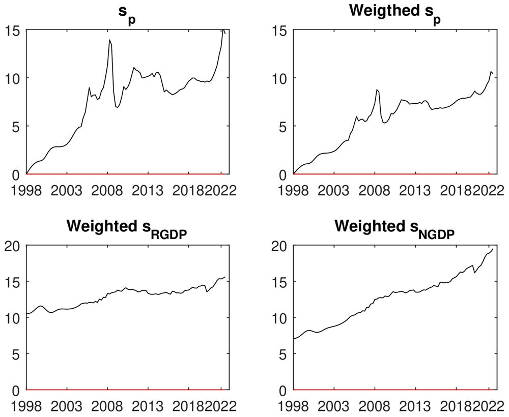
Figure 1. Estimation of the terms of trade for the US.
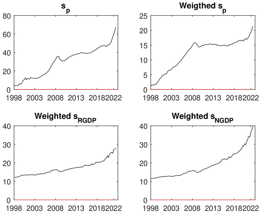
Figure 2. Estimation of the terms of trade for the EA.
Comparing the first two plots in Figure 1 shows how, thanks to weighing the size of each state/country with respect to the union, the statistics are lower and less volatile. In both cases, the dispersion grew quickly during the first years because of the existence of a base year. If 1970 or 1980 could be used as the base year, this effect would be eliminated. Once the series arrives in 2005–2006 this effect dissipates, and the series is relatively constant and below 10. There are some relevant deviations, such as the one before the 2008 crack when the dispersion was growing and just after the crack when the dispersion fell. Once it recovers in 2012, it is relatively constant until the COVID and subsequent shortage of supplies. Overall, the weighted terms of trade computed using the price dispersion are relatively constant and bounded below 10.
A similar result can be observed if we turn our view to the second pair of plots in the above figure. Looking at the dispersion in Real GDP, it grew very slowly during the considered period. These series are less volatile than prices, and the effect of the 2008 crisis is not as clear. However, it was observed that the growth in dispersion was faster before 2008. It can also be observed that the dispersion falls after 2009–2010 like in the first and second plots. The effect of COVID is more vividly observed in the Real GDP dispersion plot than in the price plot. As above, it is observed that both the fall in the first quarters of 2020 and the rise shortly thereafter. Finally, in the last plot of the figure, roughly the same behavior as in the Real GDP is observed, but now, it fluctuates around a trend. This trend is a consequence of including inflation in our analysis. Figure 2 shows the same plots for the EA.
The first thing to note is the large difference between the first and second plots in Figure 2. The dispersion in the plot without weighting is large compared to the one where the dispersion is weighted by the size of each country; the difference in the y-axis labels should be noted. As in the US plot, the dispersion grew quickly during the first few years of the series. This bias is caused by the existence of a base year for prices in 1997. Similar to the US, this rise stopped in 2008 as a consequence of the financial crisis; however, unlike the US, the rise in EA is faster, constant, and without any relevant fluctuations. In addition, the levels of dispersion in EA were higher than those in the US. The maximum in the US is slightly above 10 in 2022, while in EA it is already above 15 in 2008. As in the US, the dispersion in the EA falls after the financial crisis of 2008, but the fall is smaller than in the US and lasts for less time. After this, it stabilizes around 2010 and remains more or less constant until the COVID and subsequent shortages supply shock.
In contrast to the US, where the terms of trade seemed to fluctuate around the mean, in the EA, it seemed to fluctuate around a trend. However, as in the US, this tendency may be caused by the existence of a base year. The best way to test the robustness of these findings is to compare them with a different statistic that does not need such a thing. As before, I plotted the weighted dispersion in the Real and Nominal GDP for the EA countries in the lower panels of Figure 2.
Looking at the GDP dispersion plots, I observe how dispersion grows for both variables during the study period. In the US, the statistic based on Real GDP grew from 10 to 15, which could just be a fluctuation around the mean; in the EA, the same statistic grew from 10 to 30; this is tripled in roughly 20 years. Something similar is observed in the statistic based on the Nominal GDP, while the plot for the US seemed to be fluctuating around a trend, in the EA it looks like the rate of growth of this statistic is accelerating.
Based on this information, it can be concluded that EA is a much more heterogeneous union than the US. In addition, I have shown that states in the US may experience some degree of divergence, but nothing comparable to that experienced by countries inside the EA. The divergence observed in EA was much faster than that observed in the US. This rising divergence in a monetary union without a common fiscal authority may put in danger the capabilities of individual fiscal authorities to stabilize their economies. To show the strong link between monetary policy and terms of trade in Table 1 I compute the correlations between them and the interest rate.
Table 1. Correlations between interest rate and terms of trade.
| sp | Weighted sp | Weighted sRGDP | Weighted sNGDP |
|---|
| rUS | −0.58 | −0.62 | −0.64 | −0.63 |
| rEA | −0.74 | −0.66 | −0.72 | −0.73 |
It can be seen that the correlation between the terms of trade and the interest rate is negative and strong, independent of how I measure the former variable. This works as a robustness check to show that the influence of the terms of trade in monetary policy determination should be considered, as I have argued using the union welfare loss function in Equation (30). This finding is consistent with the literature. For instance, see De Fiore and Liu (2002) and Obstfeld (2009), in which this relationship is broadly discussed. I then have a good reason to estimate the monetary policy rule using terms of trade as an explanatory variable.
3. Estimation of the monetary policy rule for the US and EA
The litmus test to determine the influence of the terms of trade in monetary policy determination estimates the rule for the US and the EA and determines whether this variable is significant. The first step in this process is to transform Equation (32) into regression functions:
Model 1:
Model 2:
where πt and yt are the weighted averages of output and inflation for the union, respectively, and st is the absolute value of terms of trade. It should also be noted that no intercept has been added because the model is defined in deviations with respect to the steady state.
For the US, I use quarterly seasonal and calendar-adjusted data from the Bureau of Economic Analysis (BEA) and the Federal Reserve between 1998 and 2022. For inflation, I use the annual growth of the quarterly GDP deflator; for the interest rate, I use the effective federal fund rate. For the output gap, as in Taylor (1999), I used the HP filter cycle component of the Real GDP per capita. A quarterly GDP deflator was not available for states in the US until 2005. I used cubic interpolation to estimate the quarterly data from the annual data for the period 1998–2004. In both cases, data are available at the BEA. The US data are shown in Figure 3.
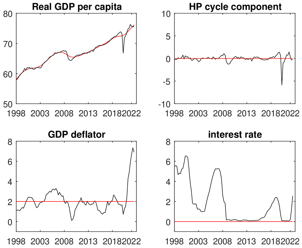
Figure 3. The first plot contains the Real GDP per capita of the US in black and the HP-filtter trend component in red.
Figure 3 shows how GDP per capita fell shortly after the crisis of 2008 and shortly after the COVID shock. I computed the potential GDP per capita as the trend component of the HP filter, which is plotted in red in the first plot of Figure. The second plot shows the cycle component of the HP-filtter is available in the second plot. In the third plot, it can be observed that inflation, measured by the GDP deflator, fluctuated around 2% in most of the current century. This fluctuation had two remarkable exceptions: the fall following the 2008 crisis and the current rise due to shortages in input supplies. Finally, in the fourth plot, we observe how the interest rate evolved during the last two decades and how it was in the neighborhood of zero for the lustrum following the 2008 financial crisis. It is observed that the interest rate fell due to the COVID crisis and the fast rise shortly after because of the supply crisis and Ukraine War.
For the Euro Area, I use quarterly Real GDP per capita and the GDP deflator from the Eurostat. The interest rate was the European Central Bank’s euribor. I use EA-19 as a representation of EA.
Figure 4 plots the same variables as in Figure 3 but for the Euro Area. In the first plot, it is observed how the deviations from the potential GDP per capita are larger in the EA than in the US. The fall in GDP per capita following the 2008 and the one following the COVID crisis observed in the US are not the only relevant deviations from its potential output. It is also observed a relevant fall on GDP per capita following the Euro Area sovereign debt crisis, an important set back in the EA recovery from the financial crisis. In the second plot of Figure 4, the cycle component of the HP-filter is provided. If our attention is turned to the GDP deflator, the plot is very similar to the one in the US. This is, inflation is around 2% in the studied period, with a rise in the last periods because of the supply shock affecting the world.
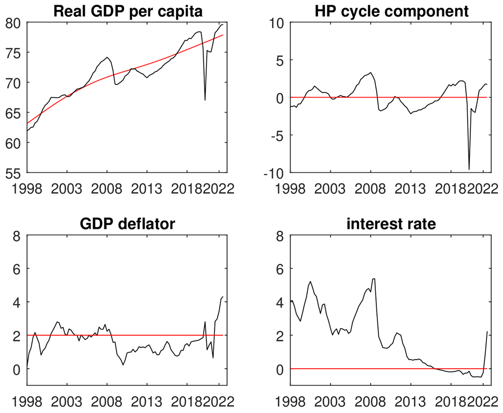
Figure 4. The first plot contains the Real GDP per capita of the EA and the HP-filtter trend component in red.
The y-axis are the same for both currency areas for consistency and comparability.
Lastly, in the fourth plot, I depict the behavior of the interest rate. Another important difference between the US and EA is that the EA interest rate fell below the 0% threshold after 2015, when the interest rate was already recovering in the US. This was one of the most important symptoms of the stabilization problems that the EA confronted when fighting the liquidity trap, which followed its sovereign debt crisis.
Until now, I have described the data, but I have not presented empirical conclusive evidence in favor of the importance of considering the terms of trade when deciding the interest rate of the union. To show the importance of this variable in monetary policy determination, I estimate the monetary policy rule (38) and modified monetary policy rule (39) using Bayesian methods. The Frequentist approach would allow for the parameter for inflation to be negative, which would be contrary to ECB and FED mandates. I then exploited the capabilities of Bayesian statistics to include a positive prior distribution for this parameter. Following the results obtained by Taylor (1999) and the monetary policy consensus, I assume the prior distribution of ϕπ to be a LogNormal(0,1). That is, before putting the model through data, I expect the influence of inflation in the interest rate to always be positive and to be, with a 95% probability, between 0.14 and 7.1%, in both monetary areas. I chose a log-normal prior distribution because both the ECB and the Fed are bound to increase/decrease the interest rate whenever their economy suffers a positive/negative inflationary shock. From an economic theory perspective, this mandate makes it impossible for the coefficient of inflation to be negative, making the log-normal distribution the most appropriate to describe this relationship. Similarly, I assumed the prior distribution for the influence of the output gap to be between -3 and 5 with a 95% probability. Thus, ϕy was assumed to have a prior distribution of a N(1,2). The effect of the terms of trade is less known, which is why I center the prior distribution around 0 and assume it to be between -4 and 4 with a 95% probability or, what is the same, I assume a prior distribution for ϕs of a N(0,2). These values are consistent with those reported by Bullard and Mitra (2002). Finally, for the interest rate, I chose a normal distribution for the likelihood, instead of using a positively bounded distribution, such as the log-normal, because the ECB has allowed for the interest rate to be negative.
Table 2 displays the results of the Bayesian estimation of the US Policy rules. In the first part of Table 2, the results of the estimation of Model 1 are presented. The results of the estimation of Model 2 are displayed in the lower part of Table I. This model is divided into two submodels, depending on which estimators of the terms of trade are used in the regression.
Table 2. Bayesian estimation of the monetary policy rule (38) for the US.
| mean | sd | 5% | 95% |
|---|
| φy | 0.55 | 0.18 | 0.25 | 0.84 |
| Model 1 | φπ | 0.64 | 0.09 | 0.49 | 0.79 |
| σ | 2.10 | 0.15 | 1.87 | 2.37 |
| WAIC | 431.4 | | |
| φy | 0.40 | 0.20 | 0.08 | 0.73 |
| Model 2.1 | φπ | 0.91 | 0.19 | 0.61 | 1.22 |
| sp | φs | −0.09 | 0.05 | −0.17 | 0.00 |
| σ | 2.09 | 0.15 | 1.86 | 2.36 |
| WAIC | 431.6 | | |
| φy | 0.39 | 0.20 | 0.06 | 0.72 |
| Model 2.2 | φπ | 0.91 | 0.19 | 0.61 | 1.23 |
| Weighted sp | φs | −0.12 | 0.07 | −0.23 | 0.00 |
| σ | 2.09 | 0.15 | 1.85 | 2.36 |
| WAIC | 431.4 | | |
Table 2 shows how the coefficients for inflation and output gap are positive and significant for the first model. If the terms of trade are not considered, by each point output deviates from its steady state equilibrium, the Federal Reserve increases interest rate in 0.55 points. In the same way, by each point inflation deviates from its objective, the Fed reacts increasing interest rates in 0.64 points. These values are low if compared with the reaction to inflation and output gaps necessary to ensure uniqueness of equilibrium computed by Bullard & Mitra (2002). If the US was modelled as a country instead of as a group of states sharing a common currency, in most of the cases, the US would not fulfil the Blanchard-Kahn conditions.
This problem disappears when terms of trade are considered. In Model 2.1, I include the terms of trade using the non-weighted statistic developed in Section 2. In Model 2.2, I used one weighted by the size of each country in the union. In both cases, when this variable is taken into consideration, the reaction of the Fed to inflation and the output gap grows sufficiently for the conditions established in Bullard and Mitra (2002) to be fulfilled. The inclusion of terms of trade in the regression allows for the separation of perturbations caused by the terms of trade on inflation and/or output stabilization policies.
The only relevant difference between Models 2.1 and 2.2 is the size of the effect of the terms of trade on the interest rate. This difference is a direct consequence of the higher volatility of the statistic, which does not consider the size of each country in the union. When I look at the comparative statistics between models, I find that the three models have almost the same values for the WAIC. Therefore, from a statistical point of view, none of the three is better than the others. Nevertheless, the omission of terms of trade may cause a problem of bias in Model 1 because of the omission of a relevant variable.
To compare the reaction of the ECB to terms of trade, I run the same regressions with the same prior distributions and time frame for the Euro Area. Table 3 shows the results of the regressions with and without terms of trade.
Table 3. Bayesian estimation of the monetary policy rule for the EA.
| | mean | sd | 5% | 95% |
|---|
| φy | 1.23 | 0.73 | 0.03 | 2.41 |
| Model 1 | φπ | 1.01 | 0.10 | 0.85 | 1.17 |
| σ | 1.76 | 0.13 | 1.56 | 1.99 |
| WAIC | 394.5 | | |
| φy | 0.74 | 0.85 | −0.65 | 2.11 |
| Model 2.1 | φπ | 1.66 | 0.15 | 1.41 | 1.92 |
| sp | φs | −0.04 | 0.01 | −0.06 | −0.03 |
| σ | 1.56 | 0.11 | 1.39 | 1.76 |
| WAIC | 371.8 | | |
| φy | 0.96 | 0.90 | −0.52 | 2.43 |
| Model 2.2 | φπ | 1.51 | 0.18 | 1.22 | 1.80 |
| Weighted sp | φs | −0.08 | 0.02 | −0.12 | −0.04 |
| σ | 1.68 | 0.12 | 1.49 | 1.89 |
| WAIC | 386.1 | | |
In the table above, it is observed that the coefficient of the output gap is only significant for the 90% confidence level in the first model. This is not an unexpected outcome, because the ECB is an inflation-targeting central bank, where output targeting is a secondary objective. Considering that the coefficient for output deviations is not significant, the EA would be on average just in the threshold of uniqueness of equilibria, following the criteria established by Bullard and Mitra (2002). This is an unexpected outcome for an inflation-targeting central bank, as it would be incapable of achieving equilibria in 50% of the cases: all cases in the interval where ϕπ is smaller than 1. However, as before, this changes when I introduce terms of trade in the regression.
Once the terms of trade are considered, the reaction of the central bank to inflation increases from 1 to 1.5/1.6 with 99.5% of the observations above 1. In other words, the uniqueness of equilibria would be guaranteed in 99.5% of the cases in the EA if ϕy is equal to zero and in a higher proportion if it is greater than zero. For this to be true, something else must be true: the coefficient for the terms of trade should not be significant, because there exists a strong fiscal authority. However, unlike the US, this is not the case for EA. The inexistence of a common fiscal authority or coordinated and strong individual authority leaves monetary policy exposed to the effects of the terms of trade.
The mandate of the ECB establishes that it must react to overall inflation in the EA and maintain it below but close to 2%. Although this mandate has a problem, it is possible for all inflation to come from a country or subset of countries, with the rest in equilibria. In a complete monetary union like the US, or in one with powerful enough individual fiscal authorities like the one described by Ferrero (2009), the stability of the economy would be a problem for fiscal authorities, and the monetary authority would react as strongly as needed to maintain overall inflation in equilibrium. This reaction pushes the economies that are in equilibrium in the union out of it to help those out of the equilibrium to their convergence path. It would then be the job of the fiscal authority to ensure the convergence of all economies to their path.
However, this is not what is happening in the case for EA. When the ECB has to decide how to react to inflation deviations, it knows that if the reaction is too strong, it may cause problems for individual fiscal authorities and put their economy out of their equilibrium path for good. Then, the higher the number of economies inside the diverging union, the weaker the ECB can react to inflation deviations. This is a big problem for economic stabilization, as the monetary policy chosen by the ECB will always be too weak to fulfil its objective in the optimal amount of time. However, if they react too strongly, some economies may be put out of their convergence path, and the integrity of the union might be doubtful, as established by Bullard and Schaling (2009).
This inability of the ECB to react properly to inflation deviations produces longer convergence paths to the equilibrium. This effect was already observed in the aftermath of the 2008 financial crisis, when the EA took much more time to recover than the US did. It is also observed in the weaker reaction of the ECB, if compared to the Fed or the Bank of England, to inflation as a consequence of shortages of supplies following the COVID and Ukraine war. The ECB has tried to solve this problem during the last decade with non-conventional monetary policies such as the LTRO. At the same time, EA policymakers tried to address it for the long run, reformulating the Stability and Growth Pact and passing new legislation to create the European Stability Mechanism to strengthen the power of fiscal authorities. However, the evidence seems to conclude that this has not been enough to revert the divergent path of EA countries.
As a consequence of the supply shock crisis and the Russo-Ukraine war, the divergence between countries is growing at an even higher rate, as the evolution of terms of trade shows. This divergence was increased by the government’s response to this inflationary shock. Some countries with sufficient fiscal muscle, such as Germany, have announced measures to fight the effects of inflation on their economies. Others with lower fiscal muscles, such as Italy and Greece, cannot follow this course of events. This divergence in the reaction only increases the actual rate of divergence and might question the existence of the euro itself.
EA countries have to accept that some sacrifices are needed to preserve the union. In the medium run, it is necessary to increase fiscal coordination, even with the loss of national sovereignty. Most importantly, in the short run, it is necessary for the EA countries to stop fiscally competing between them, as this competition only increases the already existing gap between the countries and paves the way for further divergence. It is also necessary for highly indebted fiscal authorities to be able to access enough funds to stabilize their economies under the same conditions as the rest of the economies.
4. Conclusion
In this article, I have shown how traditional monetary policy without a fiscal counterpart may be ineffective in a monetary union such as the EA. This ineffectiveness arises from the fact that the central bank only reacts to aggregate variables from the monetary union and does not consider the specific deviations of each country from its objective, which is left on the hands of the individual fiscal authorities. To put it in a real world example if, in the Euro Area, Spain has an inflation of 4% and Germany is having 1%, considering that Germany is twice the size of Spain, the Euro Area is perfectly in equilibrium around its objective of 2%. However, the Spanish economy is two points above its objective, and Germany is one point below its objective. The absence of a reaction produces an imbalance in which prices from goods produced in Spain rise faster than those produced in Germany, causing a loss of competitiveness in the former with respect to the latter.
Traditionally, this internal effect has been left aside from monetary policy because it is considered a fiscal policy matter. However, omitting terms of trade from the monetary policy rule may cause bias in its estimation. To show this, I computed the welfare loss function of a two-country New Keynesian model with a monetary policy consistent with the ECB mandate. I have shown that the welfare loss function is a function of terms of trade. Thus, the omission of a relevant variable, such as terms of trade, causes an omission of relevant variable bias in any estimation of the policy rule in a monetary union. I estimated the policy rules for the EA and the US with and without terms of trade. I have found that in the US, the terms of trade are not significant because they have fiscal authority in charge of stabilizing the economy, guaranteeing homogeneous prices in the union. On the other hand, in the EA, where such an authority does not exist, monetary policy is disturbed by this heterogeneity, making it difficult for the central bank to manage price stability. The distortion caused by the terms of trade in the EA reduces the interest rate below its optimal rate, leaving longer convergence paths than in the US.
To solve the problem of multiplicity of equilibria, stronger financial integration is required. Without the loss of national sovereignty, a simple way to do this would be to redefine the concept of price stability. Currently, price stability is defined as a constant growth of prices, but it could be changed to a homogeneous constant growth of prices. With this modification, the ECB could argue for the need to intervene in the bond market of certain economies as part of its mandate to maintain price homogeneity. With this modification of the definition of price stability, the ECB could buy/sell assets from a particular country to push inflation up or down as needed, guaranteeing the homogeneity of prices in the common market. In addition, if the ECB mandate comprises buying sovereign debt of certain countries in distress, the individual fiscal authorities would be powerful enough to stabilize their economies without the need of EA countries to lose sovereignty, creating a common fiscal authority. The downside of this proposal is that some countries will be constantly indebted to the ECB and the rest of the union. However, this seems to be a low price to pay to maintain the integrity of the Euro. If no new convergence measures are established in the EA, the divergence will continue and the existence of the Euro as a currency will be at stake.
Ethics and consent
Ethical approval and consent were not required for this study.
Data availability
All data underlying the results presented in this article are publicly available under open licences permitting reuse.
All datasets are freely available and distributed under open licenses permitting reuse (CC-BY or equivalent, depending on the source). These datasets can be used to replicate the analyses and findings presented in this article.
Faculty Opinions recommendedReferences
- Batini N, Levine P, Pearlman J:
Indeterminacy with in ation-forecast-based rules in a two-bloc model. 2004. Publisher Full Text
- Batini N, Pearlman J:
Too much too soon: instability and indeterminacy with forward-looking rules. Technical report, External MPC Unit Discussion Paper, 2002. Reference Source
- Benigno P:
Optimal monetary policy in a currency area.
J Int Econ.
2004; 63(2): 293–320. Publisher Full Text
- Board of Governors of the Federal Reserve System (US): Federal funds effective rate. [Dataset]. 2023. http://www.doi.org/10.5281/zenodo.17530727
- Bullard J, Mitra K:
Learning about monetary policy rules.
J Monet Econ.
2002; 49(6): 1105–1129. Publisher Full Text
- Bullard J, Schaling E:
Monetary policy, determinacy, and learnability in a two-block world economy.
J Money Credit Bank.
2009; 41(8): 1585–1612. Reference Source
- Clarida R, Galı́ J, Gertler M:
A simple framework for international monetary policy analysis.
J Monet Econ.
2002; 49(5): 879–904. Publisher Full Text
- De Fiore F, Liu Z:
Openness and equilibrium determinacy under interest rate rules. 2002. Publisher Full Text
- ECB: The ECB's monetary policy strategy. 2003. Reference Source
- European Commission: Early leavers from education and training — quarterly. Eurostat, [Dataset]. 2023a. http://www.doi.org/10.2908/IRT_EURYLD_Q
- European Commission: Population and employment – National account. Eurostat, [Dataset]. 2023b. http://www.doi.org/10.2908/NAMQ_10_PE
- European Commission: Quarterly national accounts – GDP (output, expenditure and income). Eurostat, [Dataset]. 2023c. http://www.doi.org/10.2908/NAMQ_10_GDP
- Eurostat: Harmonised Index of Consumer Prices (HICP). Methodogical manual. Eurostat, 2018. Reference Source
- Faia E, Monacelli T:
Optimal monetary policy in a small open economy with home bias.
J Money Credit Bank.
2008; 40(4): 721–750. Publisher Full Text
- Ferrero A:
Fiscal and monetary rules for a currency union.
J Int Econ.
2009; 77(1): 1–10. Publisher Full Text
- Gali J:
Monetary policy, inflation, and the business cycle: an introduction to the new Keynesian framework and its applications. Princeton University Press, 2015. Reference Source
- Gali J, Monacelli T:
Monetary policy and exchange rate volatility in a small open economy.
Rev Econ Stud.
2005; 72(3): 707–734. Publisher Full Text
- Ida D:
Optimal monetary policy rules in a two-country economy with a zero bound on nominal interest rates.
The North American Journal of Economics and Finance.
2013; 24: 223–242. Publisher Full Text
- Mendoza EG:
The terms of trade, the real exchange rate, and economic fluctuations.
Int Econ Rev.
1995; 36(1): 101–137. Publisher Full Text
- Obstfeld MM:
International finance and growth in developing countries: what have we learned?
IMF Sta Papers.
2009; 56(1): 63–111. Reference Source
- Pappa E:
Do the ECB and the fed really need to cooperate? Optimal monetary policy in a two-country world.
J Monet Econ.
2004; 51(4): 753–779. Publisher Full Text
- Rotemberg JJ, Woodford M:
Interest rate rules in an estimated sticky price model. In: Monetary Policy Rules. University of Chicago Press, 1999; 57–126. Reference Source
- Taylor JB:
A historical analysis of monetary policy rules. In: Monetary Policy Rules. University of Chicago Press, 1999; 319–348. Reference Source
- U.S. Bureau of Economic Analysis: SQGDP1 State quarterly Gross Domestic Product (GDP) summary. [Dataset]. 2023. http://www.doi.org/10.5281/zenodo.17530727
- U.S. Bureau of Labor Statistics: Population Level. Federal Reserve Bank of St. Louis (FRED). [Dataset]. 2023. http://www.doi.org/10.5281/zenodo.17530727
- Woodford M:
Interest and prices: foundations of a theory of monetary policy. Princeton University Press, 2003. Reference Source