First, the overall method including the interaction between the JointTracker and a newly developed deep learning based I2S orientation calibration is described. Then, the different aspects of the I2S orientation calibration are detailed.
3.1 Overall method
Figure 2 illustrates the overall method, with two interacting components, (1) the skeleton tracking comprising all tasks related to model-based estimation of IMU and segment poses, with the core part being the JointTracker according to (Taetz et al. 2025) (light blue box) and (2) the I2S orientation calibration comprising all tasks related to deep learning based prediction of I2S orientations (light green box). The data exchanged by the two components is shown between the boxes (IMU poses, IMU-centered joint positions, and I2S orientations), and the inputs (IMU data) and outputs (segment poses) of the complete method are annotated on the left side of the figure.
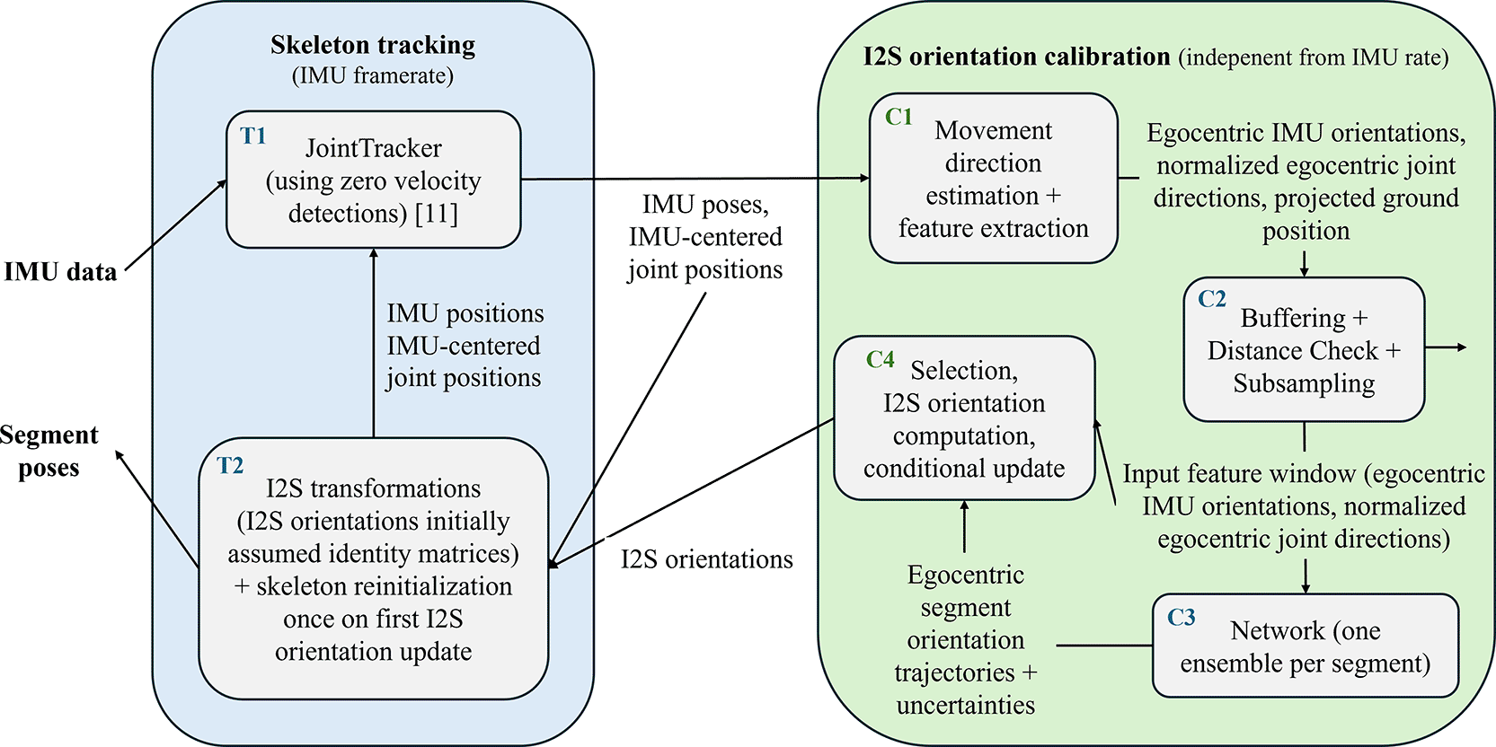
Figure 2. Illustration of the overall method.
Note, while skeleton tracking runs on IMU frame rate to deliver segment poses with minimal delay (and the currently best available I2S poses), I2S orientation calibration runs independently, on a lower rate, and it delivers I2S orientations only, if updates are available.
In the figure, the arrows indicate the data (or extracted information) flow to arrive from IMU data at segment poses. The gray boxes within each component indicate the necessary tasks, with (dark blue) labels
for skeleton tracking step
and (dark green) labels
for calibration step
. The different steps are described in the following, with the item labels corresponding to the task labels in the figure:
•
T1: Synchronized IMU data at time
are processed by the JointTracker (according to (Taetz et al. 2025) with zero velocity detections and randomly initialized joint positions). This provides IMU poses for each IMU
and IMU-centered joint positions for each joint
for time
.
•
T2: Initially assuming identity matrices for the I2S orientations of all segments, and updating those with I2S orientations (per segment) received from the I2S orientation calibration, segment poses are calculated from the estimated kinematic data using Equations (1), (2) and (5). Note, together with
, this solves the task described in
Section 2.2 after completed self-calibration. However, on the first complete I2S orientation update (i.e. once all I2S orientations have been updated at least once), the I2S orientations and IMU orientations are used together with assumed standard segment lengths (according to
meter height and the anthropometry in (Tilley and Dreyfuss 2001)) and assumed segment-centered IMU positions (IMUs sitting in the middles of the segments) to recompute the IMU positions and IMU-centered joint positions and reinitialize those states in the JointTracker. Note, this is only done once with the first updated I2S orientations to speed up convergence of the joint position estimates, since these are randomly initialized to start with.
•
C1: The first task for I2S orientation calibration is to extract suitable input features for I2S orientation prediction from the kinematic data provided by
. These features need to contain sufficient information for the task, but at the same time be invariant against irrelevant conditions such as global movement direction or segment lengths. The steps to achieve this are described in the following (cf.
Figure 1):
1. Global joint positions
are computed for each
by averaging the results of (3) and (4).
2. The current pose of the egocentric reference frame
w.r.t.
is estimated from the global joint positions. The construction is based on computing a 2D projected ground position and estimating the current movement direction of the tracked kinematic chain. The details are further described in
Section 3.2. Note, this subtask requires access to the kinematic data of the previous time
, i.e. a small buffer, which is omitted in the figure for better readability.
3. All global IMU orientations
are transformed into the egocentric reference frame
. These are denoted egocentric IMU orientations in
Figure 2, and they are represented as six-dimensional vectors
, as introduced in
Section 2.1.
4. Normalized joint directions are calculated from the global joint positions for each joint pair
according to Equation (7). The resulting vectors are rotated into the egocentric reference frame
and are denoted
(normalized egocentric joint directions).
•
C2: Since I2S orientation prediction requires some contextual motion information to reduce ambiguity, the features computed for time
(egocentric IMU orientations, normalized egocentric joint directions) are buffered and resampled to construct
(one per IMU) suitable input feature windows (motion segments) with
samples (in the experiments, 60 samples corresponding to 1 second of 60 Hz data are collected in a sliding window, each window is subsampled to 10 samples). Moreover, using the corresponding 2D projected ground positions from the previous step, a distance check is performed on a motion segment before passing this on to the next step (in the experiments, motion segments showing a traveled distance of less than 0.5 meters are omitted). This avoids predictions from uninformative input features.
•
C3: This is the core of the I2S orientation calibration, where each feature window
provided by
with
samples comprising the egocentric IMU orientations of IMU
and normalized egocentric joint direction vectors of all joint pairs
is used to predict a motion segment of
egocentric segment orientations and uncertainties (variances) via sequence-to-sequence prediction from the previously trained ensemble network to obtain:
(8)
Here,
denotes the six-dimensional continuous orientation representation introduced in
Section 2.1,
represents the training data with inputs
and labels
. The inputs are (as mentioned above):
- IMU orientation sequence:
and the corresponding
- Joint direction sequence:
.
The prediction (predicted normal distribution)
equals:
(9)
Here,
is a six- dimensional diagonal matrix
(10)
with variances
, as predicted by the ensemble network, based on (
Lakshminarayanan, Pritzel, and Blundell 2017). The network structure and training routine are detailed in
Section 3.3. Note that an individual ensemble network is trained for each segment (i.e. the predictions are per segment), while the input feature vector for segment
contains IMU orientations of IMU
and of all joint directions in the kinematic chain. Within the input features, the joint directions provide information about the egocentric segment pose, which helps the network to discriminate between I2S orientation and segment orientation variations.
•
C4: This task stores the best available I2S orientations and associated uncertainties (initialized with infinity) for all segments. When a new prediction is available from
, per segment
, from all
predicted egocentric segment orientations, the sample
with the lowest uncertainty (lowest maximum variance over orientation parameters at time
) is selected, and, together with the corresponding input egocentric IMU orientation, this is used to compute a new I2S orientation
. Here, the rotation matrices are reconstructed from the six-dimensional representations using the cross product. For each segment, if the current uncertainty is smaller compared to the stored one, the new I2S orientation is stored with uncertainty. New I2S orientations are provided to
.
Note, for the complete method, once self-calibration has completed, in order to reduce the computational burden, the JointTracker can be replaced by the tracking method proposed in (Miezal, Taetz, and Bleser 2017) (without joint center estimation) using the calibrated I2S transformations. In the current implementation, self-calibration is considered as completed, if all IMU-centered joint position estimates have converged according to the convergence indicator proposed in (Taetz et al. 2025).
3.3 Deep learning based IMU-to-segment orientation prediction with uncertainties
After shortly summarizing the mathematical background of Deep Ensembles, first, the inference with uncertainties is described, then the training data generation, network architecture and training are detailed.
3.3.1 Deep Ensembles
To obtain reliable predictive uncertainties, we adopt Deep Ensembles (Lakshminarayanan, Pritzel, and Blundell 2017) and model the conditional predictive distribution for a target vector
given an input
as a Gaussian
(13)
where
denotes the training set. An ensemble consists of
neural networks
with parameters
, trained independently (different initializations and data shuffling). Each network outputs (1) a mean vector and (2) a diagonal (heteroscedastic) covariance:
(14)
with
and
the log-variances. The predicted diagonal covariance of network
is
(15)
which represents aleatoric uncertainty (input-dependent noise) (
Kendall and Gal 2017).
Training objective. Each ensemble member is trained by minimizing the negative log-likelihood under a Gaussian noise model (heteroscedastic regression). For training pairs
, the loss for member
is
(16)
Since
is diagonal, this corresponds to a weighted squared error plus a regularizer on the predicted variances, and the aleatoric uncertainty is learned implicitly (no uncertainty labels required) (Kendall and Gal 2017).
Predictive mean and variance (Gaussian mixture moments). At test time, the ensemble defines a mixture of Gaussians. We approximate it by a single Gaussian via moment matching. The predictive mean for an input
is
(17)
and the predictive covariance is
(18)
Thus,
captures both average aleatoric uncertainty and epistemic uncertainty via the disagreement between ensemble members (Lakshminarayanan, Pritzel, and Blundell 2017). In our implementation we retain only the diagonal entries of
, consistent with the diagonal output parameterization.
3.3.2 I2S prediction per motion segment
As already described for task
in
Section 3.1, orientation prediction requires contextual motion information to reduce ambiguity. Therefore, the per-timestep features computed at time
(egocentric IMU orientations and normalized egocentric joint directions) are buffered into sliding windows and resampled to construct, for each IMU/segment
, an input feature window (motion segment) of length
. In the experiments,
samples (corresponding to
second at
Hz) are collected and then subsampled to
samples per window. In addition, using the 2D projected ground positions from the previous step, we apply a distance check and omit windows with traveled distance below
m, which avoids predictions from uninformative motion.
Per segment ensemble predictor. We train an individual Deep Ensemble for each segment
. The resulting ensemble predictor
maps the windowed input sequences to a distribution over a sequence of egocentric segment orientations, with the symbols being introduced already with
Equations (8) to (10):
(19)
The output is a per-time step Gaussian distribution
(20)
where
and
is diagonal. Both are obtained by deep ensemble moment matching, introduced in
Equations (17) to (18) applied at each timestep
.
Why sequence-to-sequence instead of direct I2S prediction. Rather than predicting a single I2S rotation directly from the full window (as in direct approaches (Zimmermann, Taetz, and Bleser 2018; Zuo et al. 2025)), we cast the task as sequence-to-sequence prediction and estimate an egocentric segment orientation distribution for each timestep. Empirically, direct window-to-one-rotation regression yielded higher predictive variances and less reliable predictions, especially for motions underrepresented in the training set. In contrast, the per-timestep distributions typically provide more homogeneous uncertainty behavior and enable robust selection of informative timesteps for I2S extraction. The most confident I2S rotation is then extracted from the predicted distribution as described for task
in
Section 3.1.
3.3.3 Network Architecture
Each ensemble member uses the same sequence-to-sequence architecture as depicted in
Figure 3. The design reflects that the input contains
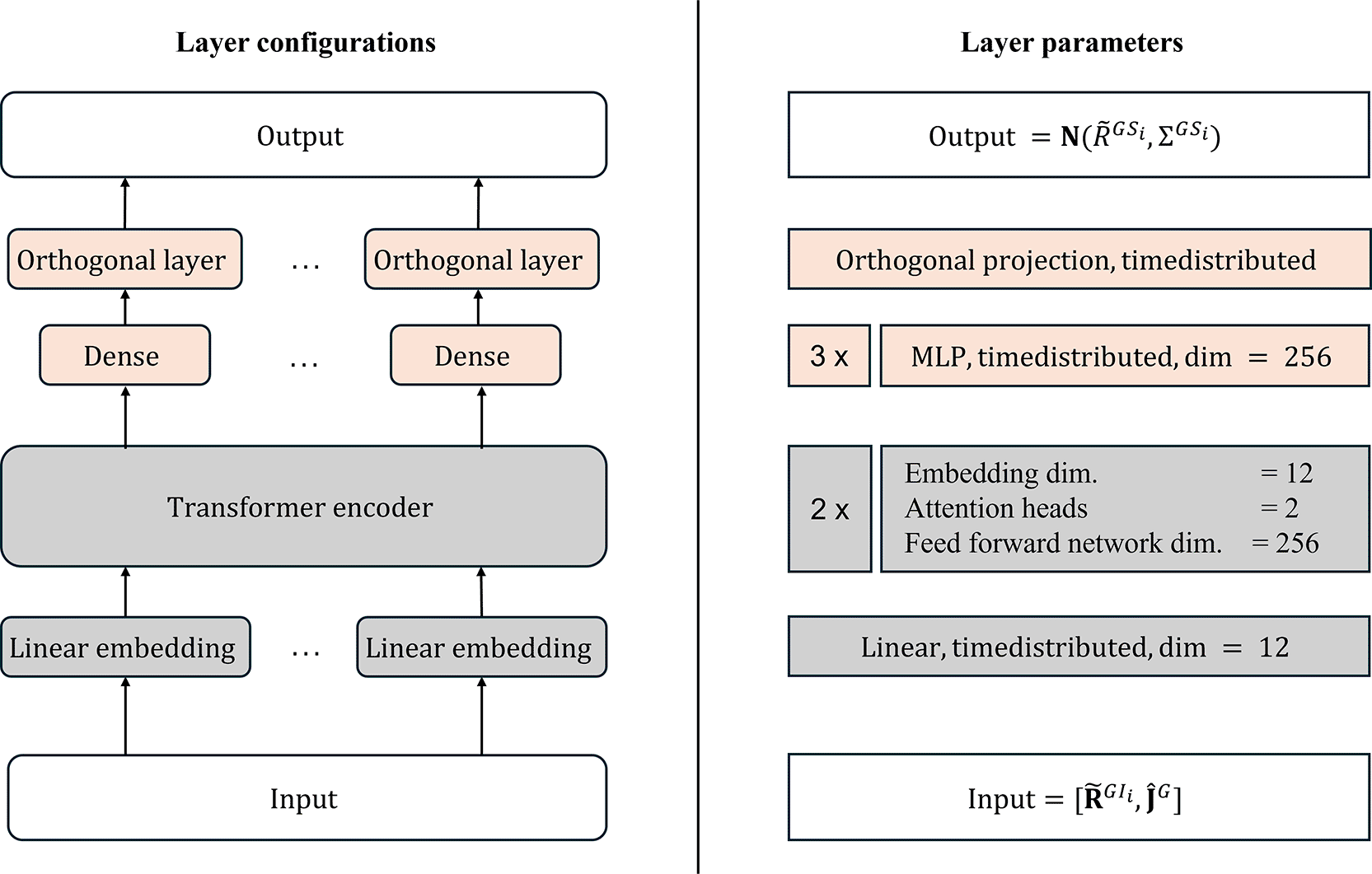
Figure 3. Network architecture with the layer configuration (left) and the corresponding parameters (right).
The orange-colored boxes model the time-constant parts, and the gray colored boxes model the time-varying parts.
Concretely, for each timestep, the input features are first linearly projected into an embedding space. We add sinusoidal positional encodings and process the sequence using a stack of Transformer encoder blocks (Vaswani et al. 2017) to model temporal dependencies. The Transformer outputs are passed through a time-distributed Multilayer Perceptron (MLP) head (three fully connected layers) that produces, at each timestep, (1) the mean of the 6D rotation representation and (2) the corresponding log-variances. Finally, we apply an orthonormalization layer as in (Zhou et al. 2019) to ensure valid 6D rotation outputs (two orthonormal
-vectors), consistent with the representation used in task
.
For each segment/IMU
we use an ensemble of
independently trained networks and compute the per-timestep predictive mean and covariance via deep ensemble moment matching, see (17, 18) or (Lakshminarayanan, Pritzel, and Blundell 2017).
3.3.4 Data preparation and network training
Our training methodology employs a self-supervised approach requiring only a dataset of global segment kinematics, specifically global segment orientations and joint positions, as input data. The kinematic chain definition used must remain consistent between the training phase and subsequent inference operations. In our experimental setup, we utilized the lower body kinematics from the musculoskeletal model described in (Rajagopal et al. 2016), with
segments/IMUs.
Data format. During the training process the input consists of motion sequences of fixed length
, comprising an egocentric 6D IMU orientation
and normalized egocentric joint direction vectors
for each time step. When concatenated and stacked, the input for a single motion sequence is represented as
. As already mentioned for task
in
Section 3.1, in our experiments we set
, corresponding to sub-sampled data from one second of kinematic recordings at
Hz by a factor of 6, effectively simulating data recording at
Hz. Each motion sequence had an overlap of
samples, equivalent to online buffering at
Hz.
Training setup. All experiments were conducted on an AMD Ryzen
processor with an NVIDIA RTX
GPU. The network ensemble was implemented in Tensorflow
and CUDA
. The training batch size was configured to
with an initial learning rate of
utilizing AdamW optimzer with default parameters. The model was trained for
epochs, with evaluation performed after each epoch to select the best-performing model as the final output.
Algorithm 1 outlines the process for generating training data from a single segment sequence. The algorithm operates in a sliding window fashion over the kinematic data input. Notably, in Experiment
, we extended our approach through simple transfer learning by fine-tuning the best-performing model on new simulated datasets (cf.
Section 4.2).
Algorithm 1. Training data generation.
01: Input: Data sequence of global segment kinematics (global segment orientations, global joint positions) with
samples (timesteps).
02: Output: Training data sets
with inputs (motion segments with
egocentric orientations of IMU
and
egocentric normalized joint direction sequences) and corresponding outputs (motion segments with
egocentric orientations of segment
) for each segment
.
03:
04:
, for all
05: while t < N −
do
06: Collect a window of
global segment orientations and joint positions (
).
07: Construct egocentric frame
from the joint positions according to
Section 3.2.
08: for each sample in the window do
09: Compute egocentric segment orientations for each segment
.
10: Compute egocentric normalized joint direction vectors according to
in
Section 3.1 and (7).
11: end for
12: if distance check fails (C2 in
Section 3.1) then
13:
14: continue
15: end if
16: for each segment
do
17: Create an output motion segment with
egocentric orientations for segment
.
18:
function
SIMULATE I2S ORIENTATIONS
19: Generate
uniform random samples on a unit sphere and construct the respective normals as
-vectors (
in the experiments).
20: for each random sample do
21: Generate
I2S orientations by aligning the virtual IMU coordinate system’s
-axis (
) with the sampled normal and adding
rotations around the normal, each by an angle of
degrees (
in the experiments).
22: end for
23: Reject new orientation samples, which are too close to a previous sample (
in the experiments).
24: return Simulated I2S orientations (
)
25: end function
26: for each simulated I2S orientation do
27: Compute the
egocentric IMU orientations for (virtual) IMU
according to (1).
28: Create an input motion segment from the egocentric IMU orientations and the above constructed egocentric normalized joint direction vectors. Note, while the egocentric IMU orientations are different for each simulated I2S orientation, the normalized egocentric joint directions are the same, representing the body pose. This enables better discrimination between I2S orientation variation and motion as compared to relying purely on the egocentric IMU orientations alone. Note that we do not include direct IMU sensor information as input features (in contrast to (
Zimmermann, Taetz, and Bleser 2018), (
Zuo et al. 2025)) to allow for training data generation from any kinematic chain sequences.
29: Add the input and output motion segments to
.
30: end for
31: end for
32:
33: end while
34: return
for all









