To complement the analysis with an applied perspective, we present an extended case study inspired by our previous work (Pietri et al. 2025), illustrating how event-aware forecasting can support proactive orchestration and predictive capacity management in mobile edge networks. While our previous study explored traffic prediction with recurrent models and exogenous web signals, here we broaden the analysis to compare multiple forecasting strategies—from naïve persistence to classical machine learning to recurrent and PatchTST-style Transformer models—and assess their impact under capacity-constrained orchestration scenarios.
Figure 2 summarizes the pipeline to forecast network demand in our case study.
Experimental design
The experimental workflow couples one-hour-ahead traffic forecasts with a simplified retrospective capacity benchmark. The purpose of this benchmark is to quantify how forecast-informed provisioning can reduce traffic exceeding a fixed reference capacity. It is not intended to reproduce a complete RAN, core-network, or operator resource-allocation process.
Each spatial node is evaluated through its service-cluster traffic series. We assume a simplified monotonic relationship between observed traffic volume and required capacity and abstract away detailed radio scheduling, handover dynamics, compute placement, and nonlinear resource-consumption effects. This abstraction allows forecasting methods to be compared under a common capacity-constrained criterion without introducing network-topology assumptions that are not available in NetMob’23 dataset.
For the operational evaluation, static reference capacities are defined from the 70th, 80th, and 90th percentiles of the observed demand in the evaluation block. Forecast-informed capacity can increase above the corresponding static reference when predicted demand requires it. Performance is then quantified through the relative reduction in overload with respect to the static-capacity benchmark, as formally defined below.
This operational benchmark should therefore be interpreted as a retrospective proxy for under-provisioning risk. It does not directly estimate operator capex, energy consumption, RAN scheduling efficiency, or end-to-end performance in an operational 5G/6G deployment. We assume that mobile traffic generated by base stations (BSs) is classified into multiple service categories. Network resources within each node are partitioned across several network slices, with each slice dedicated to a distinct service class. For example, a slice dedicated to video services handles all corresponding traffic flows. This model abstracts from specific network components, such as distinctions between radio access network (RAN) and 5G core functions (e.g., data plane versus user plane), given the lack of detailed configuration data and the broader conceptual focus of the study.
Although simplified, this architecture is sufficiently general to represent a wide range of modern network deployments. By focusing on traffic flows and resource distribution across slices and hierarchical levels, the model supports scalable simulations and theoretical evaluations—both of which are critical for network planning and performance optimization (see
Figure 3).
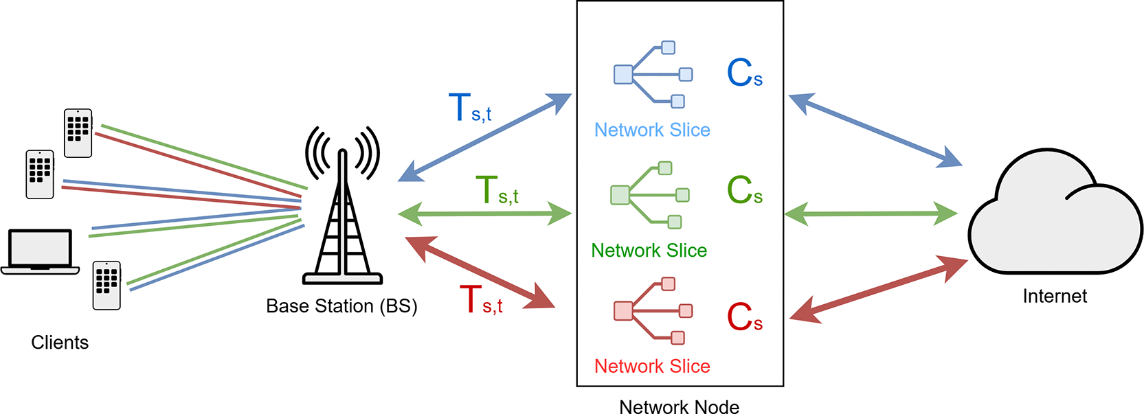
Figure 3. Model of the network.
A network node serves the traffic from a given geographical area. Multiple network slides are instantiated to match requirements of different classes of services. Traffic for a given slice s at a given time t is represented by Ts,t. Slice capacity is represented by Cs. The network goal is to minimize the time and the magnitude of excess load (Ts,t > Cs) while minimizing the sum of Cs (as it entails capex for the telecom operator).
Event-aware feature engineering. The forecasting models use endogenous traffic features and, when enabled, exogenous event-aware features. Endogenous inputs consist of lag1–lag24 together with hour-of-day and day-of-week encodings.
Event-aware inputs are derived primarily from scheduled-event records and include event_active, event_count, event_intensity, event_relevance, event_before, event_after, event_temporal_proximity, event-type indicators, and a public-holiday indicator. Event records are aligned with the hourly traffic index; events spanning multiple hours remain active over the corresponding intervals, while before/after and temporal-proximity variables represent the periods surrounding each event. Missing event-related values are encoded as zero.
The same event-aware feature construction is used across forecasting models. In the no-event ablation, only these exogenous variables are removed, while traffic lags and regular temporal encodings remain unchanged.
Google Trends and social-media streams are treated as optional contextual sources in the broader pipeline. For the historical 2019 case study, web/search information, where used, was obtained retrospectively; the experiments therefore do not establish that such signals would have been available with the same timing in a live forecasting system. The primary reproducible event-aware inputs are scheduled-event records and their derived temporal indicators.
For each model, the same event-aware feature set was used when exogenous variables were enabled. The ablation experiment reported in
Figure 6 was obtained by removing all event-related variables while keeping the endogenous traffic lags and temporal encodings unchanged. This ensures that the comparison isolates the contribution of event-awareness from the contribution of regular temporal seasonality.
Models and training setup. The comparative evaluation involves five representative forecasting families, selected to cover a progressive spectrum of model complexity and learning capacity:
• Naïve: a persistence baseline assuming y(t) = y(t-1). This model has no trainable parameters and serves as a lower-bound reference.
• Ridge: a linear autoregressive model with Ridge regularization, using lagged traffic values, hour-of-day indicators, day-of-week indicators, and event-aware features when enabled. The regularization strength was selected on the training data.
• Random Forest: a non-parametric ensemble capturing nonlinear interactions between temporal, service-level, and event-aware features. The model was trained using the same input feature set as Ridge.
• LSTM: a recurrent neural network with memory cells (Hochreiter and Schmidhuber 1997), modeling temporal dependencies in service demand. The LSTM models used the same chronological training/test split as the other baselines and were trained with early stopping to prevent overfitting.
• PatchTST-style Transformer: a lightweight patch-based Transformer baseline inspired by recent time-series forecasting architectures. The model segments the input history into temporal patches and applies a Transformer encoder to capture longer-range temporal dependencies.
The split is chronological and the forecast horizon is one hour. The final 20% of each post-lag series is held out as the contiguous test block. Within the preceding 80%, the final 20% is reserved as validation for model selection and early stopping, corresponding to an effective 64%/16%/20% train/validation/test partition of the supervised samples. For a complete hourly series spanning 17 March-31 May 2019, the 24-hour lag warm-up yields approximately 18 March-4 May for training, 5–16 May for validation, and 17–31 May for testing. No test observation is used by Optuna. For the PatchTST-style baseline, we used the same node-level forecasting setup and the same event-aware input variables adopted for the other models. The model used a 24-hour input context, patch length 6, stride 3, d_model = 64, 4 attention heads, 2 Transformer encoder layers, and dropout = 0.10. Training was performed with AdamW, learning rate 10^−3, weight decay 10^−4, batch size 32, and early stopping on a validation split of the training set. The PatchTST-style model was evaluated using the same accuracy and orchestration metrics as the other forecasting models.
LSTM settings are selected globally on a deterministic subset of nodes and then reused across clusters.
• LSTM opt_std: one LSTM layer, MAE training loss and Adam optimization. Optuna varies the number of LSTM units (50–500), maximum epochs (50–500), batch size (2–128), and learning rate (10^-5–10^-1, logarithmic scale). Trials are ranked by validation RMSE; the full search comprises 1000 trials.
• LSTM opt_cst: the same recurrent search space, but trained with the asymmetric direction-aware provisioning loss defined below. The network is trained on per-node MinMax-scaled targets and model selection uses the validation partition; the final test block remains untouched until evaluation.
Asymmetric loss. Following (Bega et al. 2019, 2020), we employ a customized direction-aware, piecewise loss function. Let e = P −T denote the signed prediction error, where e < 0 corresponds to underprediction. The loss function is parameterized by α ∈ (0, 1), ϵ > 0, K ≥ α, δ > 0, η ∈ (0, α), and tail width ∆ > 0. We define the threshold parameter eend, the slope msh, and the smooth transition function σ(z) as:
The asymmetric bounded loss L(e) is then defined piecewise as:
The construction is continuous and bounded in [0, K]. Underprediction receives a high penalty, moderate positive error enters a lower-cost shoulder, and large overprediction is penalized again through the smooth tail. Thus, the objective expresses the operational preference for avoiding service shortfall without making unbounded overprovisioning cost-free. The loss parameters are interpreted in normalized target space, and their defaults/search ranges are recorded by the released code.
The asymmetric objective is not expected to minimize RMSE. Its intended effect is to alter the residual distribution by making under-prediction more costly than moderate over-prediction. Accordingly, the analysis separates symmetric accuracy from direction-specific behavior. In addition to MAE, RMSE, MAPE, and R2, the released evaluation code exports under-prediction rate and magnitude as well as corresponding over-prediction diagnostics on the original target scale. The main comparison below therefore interprets the asymmetric objective through both its conventional forecasting metrics and the operational overload benchmark, without assuming that it must improve every symmetric error measure.
Operational metrics. Forecast accuracy was measured through Mean Absolute Error (MAE), Root Mean Square Error (RMSE), Mean Absolute Percentage Error (MAPE), and coefficient of determination (R2). Operational performance is assessed through a retrospective overload-reduction benchmark. For each capacity level q∈{0.70,0.80,0.90}, the static capacity Cq is defined as the q-th percentile of the observed demand in the evaluation block. Given observed demand Tt and forecast Pt, forecast-informed capacity is defined as
respectively. Relative overload reduction is then
We report OR@70, OR@80, and OR@90 as percentages relative to the corresponding static-capacity benchmark. This metric is a retrospective operational proxy and is not interpreted as a direct estimate of capex, energy consumption, or live-network performance.
Event-input robustness protocol. To isolate uncertainty in the exogenous event information, the observed traffic series, held-out targets, and trained model weights are kept fixed while only the event calendar is perturbed within the evaluation block. Because only three perturbable scheduled events occur in that block, percentage severities would collapse to identical integer counts; the experiment therefore uses absolute counts. The 27 factorial conditions combine 0, 1, or 2 cancelled event records; 0, 1, or 2 spurious event records inserted into originally event-free periods; and temporal displacements of 0, 1, or 2 hours applied to selected surviving events. Public holidays are kept deterministic. After every perturbation, all derived event features are regenerated before inference. Results are reported as changes relative to the clean C0/FP0/SHIFT0 condition, so the experiment measures event-input sensitivity rather than changes in realized demand.







