1. Introduction
The global transition to renewable energy has increased the call for efficient and reliable power forecasting systems. Among all renewable resources, wind stands out because it is cheap, scalable, and ubiquitous. Nevertheless, its nonlinear and stochastic nature, caused by atmospheric turbulence, meteorological randomness, and turbine dynamics, poses strict challenges to market operations and grid stability. Accurate wind power forecasting thus becomes important to maximize scheduling, balance energy supply and demand, and maintain overall grid stability.
Statistical models and traditional machine learning models such as Linear Regression (LR), Polynomial Regression (PR), and Support Vector Machines (SVMs) have been found to be successful for short-term forecasting tasks as they are easy to interpret and use. However, these models are prone to making linear inferences and are poor at capturing the nonlinear, complex relationships between power output, turbine output, and wind speed. As noted in recent reviews, the internal variability of wind speed and its nonlinear mapping into output power make classical models unsuitable for consistent performance under weather variability.i,ii,iii
To transcend these limitations, nonlinear and kernel-based methods, including SVR and deep neural networks, have been widely utilized. Such methods can represent higher-order dependencies within the data but typically require large computing power and memory, particularly when dealing with high-resolution turbine data or long historical time series.iv This growing computational requirement has promoted the integration of HPC for model training and optimization, combined with edge computing, which supports localized, low-latency inference at the substation or turbine level.v The combination of edge and HPC paradigms supports a distributed intelligence architecture for renewable energy forecasting—where edge nodes provide rapid initial forecasts and HPC systems refine them with more complex modeling, including quantum-augmented approaches proposed in this research.vi
The subsequent analysis focuses on the intersection of HPC and new Quantum Machine Learning (QML) technologies for renewable energy forecasting. Quantum-enhanced methods, in particular QSVR with quantum fidelity kernels, are capable of learning intricate feature dependencies that are difficult for classical algorithms to learn. However, due to the current hardware and algorithmic limitations, purely quantum models underperform compared to optimized classical baselines. To mitigate this, we propose a hybrid HPC–Edge framework where an edge-based LR model performs early lightweight prediction, and the quantum model executes on HPC infrastructure to enhance predictions using residual learning — a process we refer to as the “help from Edge.”
The main contributions of this research are the following:
• Creating a hybrid HPC–Edge pipeline for wind power forecasting from real-world SCADA data.
• Implementing a wind power forecasting application with a QSVR that is based on a quantum fidelity kernel for enhanced feature correlation modeling.
• Proposing the concept of “help from Edge”, where the quantum model enhances edge-based predictions through residual correction.
• Providing a comparative evaluation of Edge-only, Quantum-only, and Hybrid (Edge-assisted Quantum) approaches to analyze the quantum integration benefits and drawbacks in wind power forecasting.
2. Related work
Wind power forecasting has been an active area of research for decades with numerous data-driven and traditional approaches suggested to model the complex interaction between turbine output and meteorological variables. Time-honored forecasting techniques such as LR and SVMs have been the traditional benchmarks due to their simplicity and interpretability.vii Sophisticated Artificial Neural Networks (ANNs) and ensemble methods (e.g., Random Forests, Gradient Boosting, and hybrid neuro-fuzzy networks) have demonstrated increased accuracy through the ability to capture nonlinear patterns among wind direction, wind speed, and power output.viii However, these models would involve a significant amount of computer resources and tuning, especially for large or high-frequency turbine datasets.
These computational requirements are countered by increased usage of HPC within renewable energy forecasting. Parallel and distributed paradigms have allowed enormous SCADA datasets to be handled, accelerating model training and enabling ensemble evaluation at scale. Machine learning pipelines accelerated via HPC have been shown to significantly reduce execution time across multiple studies, while keeping forecasting accuracy intact.ix The improvements notwithstanding, the majority of deployments remain restricted to traditional architectures, and the potential of quantum-enhanced computation is largely underutilized in real-world energy forecasting applications.
Quantum Machine Learning (QML) has been demonstrated to be a promising paradigm that can effectively represent difficult-to-represent correlations in classical kernel terms. Quantum Support Vector Machines (QSVM) and QSVR models apply quantum kernels to map input data into high-dimensional Hilbert spaces, which can potentially have more feature-rich representations for time-series prediction.x Early experiments in QML for energy applications—such as load forecasting, battery control, and microgrid optimization—have demonstrated concept viability but remain constrained by hardware noise, limited number of qubits, and scalability issues.xi
Conversely, the hybrid blend of Edge and HPC computing has been of interest with respect to smart grid and Internet of Things (IoT) technology. Edge computing aids in low-latency real-time processing at or near data sources, where HPC backends provide the computational capability utilized for bulk optimizations and model iteration. Hybrid Edge–HPC architectures have been put into various applications of fault detection, smart metering, and energy management systems,xii yet the merging with quantum computing is relatively untapped.
Briefly, while classical and HPC-based forecasting has come a long way, and novel advancements in QML are already promising, there is quite a research gap in combining Edge intelligence with Quantum HPC architectures for renewable energy forecasting. This gap forms the basis of the current research, where a hybrid Edge–Quantum HPC model for wind power forecasting is presented, combining linear and quantum models in residual learning to leverage the strengths of both computational frameworks.
3. Methodology
This work proposes a hybrid computational workflow combining edge-based LR and Quantum High-Performance Computing (QHPC) for wind power forecasting. The approach combines conventional efficiency at the edge with quantum-augmented learning at the HPC layer in an attempt to harness complementary strengths in both computational paradigms.
3.1 Dataset description
The dataset employed in this research is from a SCADA system of a working wind turbine in Türkiye.xiii The dataset provides measurements at 10-minute intervals, leading to more than 50,000 instances (shape: 50,530 × 5). Each instance captures essential physical variables concerning the operation of turbines and the surrounding environment:
•
Wind Speed (m/s) – measured at hub height, which is the primary input to the generation of power.
•
Wind Direction (°) – direction of the incoming wind, critical for yaw control and turbine alignment.
•
Theoretical Power (kWh) – theoretical power output according to the manufacturer at the given wind speed.
•
Date/Time – timestamp for all measurements.
•
LV ActivePower (kW) – the actual power generated by the turbine (used as target variable).
Two additional attributes were extracted from the timestamp feature: Hour and Month, to enable the models to learn diurnal and seasonal trends in wind. The resulting feature matrix consists of five predictors:
and the target variable:
3.2 Data preprocessing
Inconsistent or missing entries were discovered and removed prior to developing the models to ensure data integrity. All numerical feature values were normalized using the StandardScaler technique to normalize feature distributions and promote numerical stability during model training. This ensures that all variables, such as wind speed and theoretical power, play a proportionate role in both classical and quantum models.
To emulate the distributed edge–HPC configuration, the cleaned data was split into two:
•
HPC subset: equivalent to the historical data processed on a centralized HPC node.
•
Edge subset: equivalent to the most recent measurements that are locally available at the turbine site, emulating real-time processing and prediction.
Several experimental configurations were considered in order to evaluate the stability of the hybrid solution. The following HPC/Edge sample splits were tried: (300/100), (400/150), (500/100), (500/200), and (600/200).
Each configuration maintains the temporal order of the dataset—older samples are included in the HPC subset, and the newest samples are included in the Edge subset.
Each subset was further divided into training, validation, and testing folds for impartial model evaluation:
•
HPC subset: approximately 80% of samples for training and 20% for validation, used to train the quantum model on residual learning.
•
Edge subset: approximately 80% of samples for training and 20% for testing, used to train and test the lightweight LR model.
This decoupling enables both compute layers to operate semi-independently—mirroring real-world deployment scenarios where the edge system provides fast, local predictions, and the HPC system post-processes the predictions to learn from historical error trends.
3.3 Edge model: Linear regression
The Edge model is the foundational prediction unit, being placed directly at the turbine or local control level, where there is real-time decision-making and computation must be low-latency. Considering the computational constraints of edge devices—microcontrollers or embedded processors—LR is selected as the primary predictive model due to its simplicity, interpretability, and low memory requirements. The model predicts the linear relationship among input meteorological and operational characteristics and active power output of the turbine.xiv
The edge dataset is preprocessed locally, including normalization, time-based feature extraction (Hour and Month), and removing incorrect or missing values. Features are introduced into the LR model after standardization, and the model is trained to minimize the residual sum of squares between estimated and measured power outputs. The mathematical expression of the model is described as:
where
represents the input feature matrix,
represents the learned regression coefficients, and
denotes the residual errors.
LR principal advantage in this setting is its ability to produce interpretable coefficients that allow operators to visualize the impact that some variables (e.g., wind speed or direction) have on power generation. Secondly, its small-size computational footprint allows for rapid inference even in devices where there are no longer available resources, allowing for unbroken in-situ monitoring without needing high-bandwidth communication channels.xv
This edge-deployed model provides preliminary power estimations which can be synchronized with the central HPC or Quantum backend periodically for model update and residual adjustment. Thus, the LR model not only enables decentralized computation but also serves to mitigate data transfer loads and system robustness in distributed renewable energy systems.
3.4 Quantum HPC model: Quantum support vector regression
In conjunction with the Edge baseline, a QSVR was also implemented on the HPC platform. The QSVR extends classical SVR to the quantum domain, aiming to model complex, nonlinear relationships that are not easily defined by classical kernels. In contrast to traditional SVR models that rely on pre-specified kernel functions such as linear, polynomial, or radial basis function (RBF) kernels, QSVR replaces this with a quantum kernel derived from quantum circuit–based feature mappings. The kernel is calculated in the form of the fidelity between quantum states representing the input data so that the model can map classically encoded feature vectors implicitly into a high-dimensional Hilbert space exponentially larger than the classical counterpart.
Within the proposed QSVR approach, the model is executed in a quantum-enabled HPC environment, where kernel computation and quantum simulations are performed using quantum circuit simulators on HPC hardware. This framework employs conventional HPC hardware to simulate large-scale quantum circuits, bridging the gap until Noisy Intermediate-Scale Quantum (NISQ) hardware matures. The use of an HPC backend assures fast processing of large datasets—such as the 50,000-point wind turbine SCADA data used in this study—while maintaining quantum-level modeling accuracy.
3.4.1 Data encoding via feature maps
The first step in building a quantum kernel is encoding classical input vectors into quantum states. For each input vector
, we apply a Feature Map circuit to a 5-qubit register.
In this study, a ZZFeatureMap with reps = 1 and linear entanglement was used because it provides a shallow circuit that can encode pairwise feature correlations while still being appropriate for NISQ-era constraints.
Mathematically, the unitary transformation is:
where
are Pauli-Z operators and
are feature-dependent phases.
xvi In
Figure 1 we demonstrate a sample of the ZZFeatureMap operating on a five-feature input, showing how circuit structure encodes classical information into quantum states.

Figure 1. Example of the ZZ feature map for a five-feature input data.
This circuit maps classical data into entangled quantum states:
where
denotes the 5-qubit Hilbert space.
A shallow circuit depth (reps = 1) was deliberately chosen to maintain low circuit complexity, numerical stability, and compatibility with NISQ-era hardware.
3.4.2 Fidelity Quantum Kernel
Once the input data are encoded as quantum states via the chosen feature map, two samples
and
are compared using the Fidelity Quantum Kernel, denoted by
. The kernel is defined by the square of the inner product of the corresponding quantum states:
Here,
is a complex-valued overlap of two state vectors, and its modulus squared estimates their quantum fidelity. The more similar the two quantum states are in Hilbert space, the larger their fidelity. This is thus a data-driven similarity measure which embeds the input data implicitly into a high-dimensional feature space defined by the quantum circuit.
Unlike conventional kernels such as the Radial Basis Function (RBF) or polynomial kernels,
naturally arises as a consequence of the quantum evolution under the feature map. Such an intrinsic characteristic allows the kernel to capture nuanced nonlinear interactions between features, which can provide denser representations for learning complex dependencies in wind turbine data.
The circuit representation of the Fidelity Quantum Kernel is presented in
Figure 2, where two feature map unitaries
and
are applied sequentially on the same qubit register. The probability of measuring the ground state
determines the kernel value
.
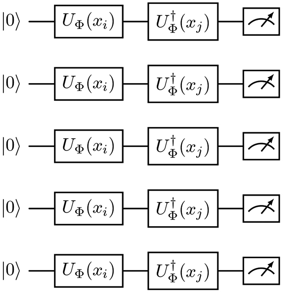
Figure 2. Fidelity Quantum Kernel circuit for 5 qubits.
Each qubit is first encoded with the unitary
corresponding to the data point
, followed by the inverse encoding
for data point
. The measurement probabilities are used to compute the kernel value
.
In order to test these fidelities in simulation effectively, the Compute–Uncompute method combined with the StatevectorSampler primitive was applied. It makes it possible to construct a general quantum circuit that is initially applied to prepare the state
, and then apply the inverse feature map
followed by measuring the ground state
probability amplitude at the end. The resulting amplitude is directly proportional to the overlap
, from which the value of the kernel
can be derived. Utilizing such kernel tests, the Quantum Support Vector Regressor (QSVR) learns the function of regression:
where
are the trained support coefficients and
is the bias term of the model. This form allows the quantum model to generalize beyond linear relationships and detect faint correlations and high-order feature interactions that may be poorly represented by the edge-based LR model.
xvii3.5 Hybrid Edge–Quantum HPC integration
To combine the best of both paradigms, a residual learning architecture is used. The integration takes place through three significant steps:
(1) Edge Prediction: The Edge LR model first generates early estimates on the HPC training set, providing a fast but coarse baseline.
(2) Residual Computation: The discrepancy between the real target values and the Edge estimates is computed as:
where
is the residual component that captures nonlinear dynamics and feature interactions unavailable in the linear model.
(3) Quantum Residual Modeling: The Quantum Support Vector Regressor (QSVR) is trained on these residuals rather than the raw targets. During inference, the final hybrid prediction is computed as the sum of the Edge forecast and the QSVR-estimated correction term:
This structure enables the quantum model to be used as a high-order correction system—capable of perceiving fine correlations and nonlinear interactions—while the Edge component is low-latency and interpretable output.xviii Together, they create an efficient, balanced hybrid system optimized for efficiency as well as precision.
3.6 Evaluation metrics
The quantitative performance of the three prediction models—Edge, Quantum HPC, and Hybrid—was compared through three standard regression metrics: Root Mean Squared Error (RMSE), Coefficient of Determination (
), and Symmetric Mean Absolute Percentage Error (SMAPE). The metrics combined provide a comprehensive assessment of prediction accuracy, stability, and relative model performance across models of different magnitude.xix
• RMSE quantifies the standard deviation of errors of prediction, reflecting how far, on average, the forecasted values deviated from actual observations. RMSE penalizes large errors more severely due to the quadratic term, and hence it is extremely sensitive to outliers. Smaller RMSE indicates higher forecasting accuracy and consistency in model performance.
• The
value quantifies the percentage of variance in the target variable accounted for by the model. It offers an interpretable measure of the quality of fit of the model in describing the underlying data patterns. A high
value near 1 implies a very good predictive fit, while negative values imply that the model is worse than a simple mean predictor.
• SMAPE is a measurement of the relative predictive accuracy as a percentage and hence magnitudes-insensitive in the target variable as well as scale-free. It adopts a symmetric definition to avoid division by small amounts that usually confounds classical MAPE and balances over- and under-predictions.xx
The three metrics are formally defined as follows:
where
denotes the true value,
the predicted value,
the mean of observed data, and
the total number of samples.
This suite of metrics provides a balanced and multidimensional evaluation framework: RMSE emphasizes absolute error magnitude,
assesses model explanatory power, and SMAPE puts relative deviation as a percentage first. Together, they ensure model comparison involves both local accuracy and global generalization capability for the Edge, Quantum HPC, and Hybrid prediction paradigms.
4. Experimental design and results
4.1 Experimental setup
Experiments were conducted with the SCADA wind turbine dataset, comprised of approximately 50,530 samples recorded at 10-minute intervals. Each record contains meteorological and operational measurements descriptive of the performance of an individual turbine over the course of several months. Input features considered are WindSpeed, TheoreticalPower, WindDirection, Hour, and Month, and the target variable is the ActivePower output of the turbine (in kW). This combination of features enables the models to capture physical and temporal dependencies required for accurate short-term power forecasting.
A data preprocessing pipeline was used prior to training the models to normalize the data and improve model convergence. Corrupted or missing entries were filtered based on turbine operational constraints, and all numerical features were normalized using StandardScaler. This normalization step normalizes the input space to have zero mean and unit variance so that the feature magnitudes are the same for both quantum and classical kernels. Moreover, normalization is particularly crucial for quantum models as the feature space is encoded as rotation angles or amplitudes in the representation of the quantum state.
The data set was divided to replicate a distributed edge–HPC computational infrastructure. The division replicates an actual deployment of hybrid renewable energy forecasting systems:
•
Edge node: A local subset of data with the most recent temporal window, which is real-time operational data available at the substation or turbine level. The Edge node executes on-premise forecasting using a light LR model to enable immediate and low-latency forecasting.
•
HPC node: A larger subset of historical data stored centrally, utilized for offline model updating and quantum-based training. This node executes QSVR with quantum kernels on high-performance computing hardware. The HPC component learns long-term temporal trends and complex nonlinear relationships not possible at the Edge level.
The partitioning strategy was developed to balance computational load while achieving temporal consistency between the two environments. The Edge model operates in continuous mode and synchronizes intermittently with the HPC node for residual updates, allowing the hybrid system to adapt to shifting wind dynamics without full retraining. All experiments were implemented in Python with scikit-learn for classical models and Qiskit Machine Learning for quantum kernel evaluation.
4.2 Evaluation methodology
This section describes the full comparison among the Edge, QHPC, and Hybrid models. The goal is to explore how different data distribution approaches among the edge and HPC components impact model performance. This analysis relies on four different experimental configurations that differ in the number of samples assigned to each of the Edge and HPC models. For all experiments, the dataset is split at the sample level using 80% of the data for training and the remaining 20% for testing. Performance is assessed by resorting to three standard metrics, namely the RMSE, the
, and the SMAPE.
4.3 Quantitative results
Table 1 reports the quantitative results across all configurations. Each setup compares three variants: (i) the Edge model, (ii) the Quantum-only model trained exclusively on HPC data, and (iii) the Hybrid model combining both approaches.
Table 1. Performance comparison of Edge, Quantum, and Hybrid models under different sample configurations.
| HPC samples | Edge samples | Model | RMSE ↓ | R2 ↑ |
SMAPE (%) ↓ |
|---|
| 300 | 100 | Edge | 171.54
| 0.9183
| 5.96
|
| | Quantum-only
| 1016.62 | −0.0546 | 35.73 |
| | Hybrid (Edge + Quantum) | 581.39 | 0.6551 | 22.43 |
| 400 | 150 | Edge | 340.86 | 0.8253 | 19.48 |
| | Quantum-only
| 2125.52 | −6.1605 | 132.37 |
| | Hybrid (Edge + Quantum) | 226.72
| 0.9185
| 63.79
|
| 500 | 100 | Edge | 171.54
| 0.9183
| 5.96
|
| | Quantum-only
| 936.13 | −1.2783 | 60.96 |
| | Hybrid (Edge + Quantum) | 413.26 | 0.5560 | 48.55 |
| 500 | 200 | Edge | 312.50 | 0.9080 | 29.42 |
| | Quantum-only
| 936.12 | −1.2783 | 60.96 |
| | Hybrid (Edge + Quantum) | 117.95
| 0.9638
| 27.00
|
4.4 Discussion
These experimental results bring to light several key understandings about the behavior of not only the Edge model but also the quantum-only HPC model and the hybrid learning framework. Overall, the evidence underlines how the classical and quantum components contribute differently to the modeling of wind turbine power dynamics and why their combination yields the best overall performance.
The Edge model consistently shows strong predictive accuracy across all configurations tested. With an
value typically greater than 0.90, the model captures the dominant linear relationships between the wind speed, theoretical power, and active power during normal turbine operation. Also, the low values of RMSE and SMAPE further suggest that the Edge model is highly suitable for fast, local inferences at the turbine level where stability and computational efficiency are crucial.
By contrast, the purely quantum QSVR, which has been trained using only the data from HPC, provides significantly weaker performance as a standalone model. Negative or near-zero
values—for example,
with 400 HPC samples—indicate that the quantum kernel struggles to learn meaningful structure from high-dimensional, unnormalized inputs. These results highlight that quantum models cannot independently handle noisy complex data distributions without some sort of preprocessing or structural guidance by classical models.
These limitations are overcome in the hybrid architecture where the quantum layer is trained to learn the residuals of the Edge model instead of the raw power output. This method yields significant performance gains compared to both independent models. Considering 500 HPC and 200 Edge samples, for example, the hybrid method attains an
value of 0.9638, beating the baseline results from an Edge-only model (
), as well as the purely quantum model (
). The hybrid performance increases from
to
in a similar fashion for the 400/150 configuration. These results show that the quantum model is especially adept at modeling complex nonlinear residual structures that a classical linear model cannot capture.
Finally, the influence of data partitioning between the Edge and HPC systems reveals that a balanced allocation of samples is beneficial. Increasing Edge-side data enhances stability and captures the dominant trends, whereas more HPC samples strengthen the quantum model’s ability to learn refined error dynamics. The best overall performance is observed for the configuration with 500 HPC and 200 Edge samples, which produces the lowest RMSE alongside the highest
value among all tested splits.
Taken together, these findings demonstrate that the hybrid model provides a synergistic interaction between classical and quantum learning mechanisms, combining the reliability of linear modeling with the expressive nonlinear structure introduced by quantum feature mappings. This makes the hybrid approach a promising direction for future high-performance wind power prediction systems.
4.5 Visualization of model performance
Figure 3 visualizes the comparison of
scores across all configurations. The hybrid model consistently surpasses the Quantum-only counterpart and, in several cases, even outperforms the Edge model. This confirms that the hybrid strategy provides complementary benefits, leveraging both local interpretability and global quantum generalization.
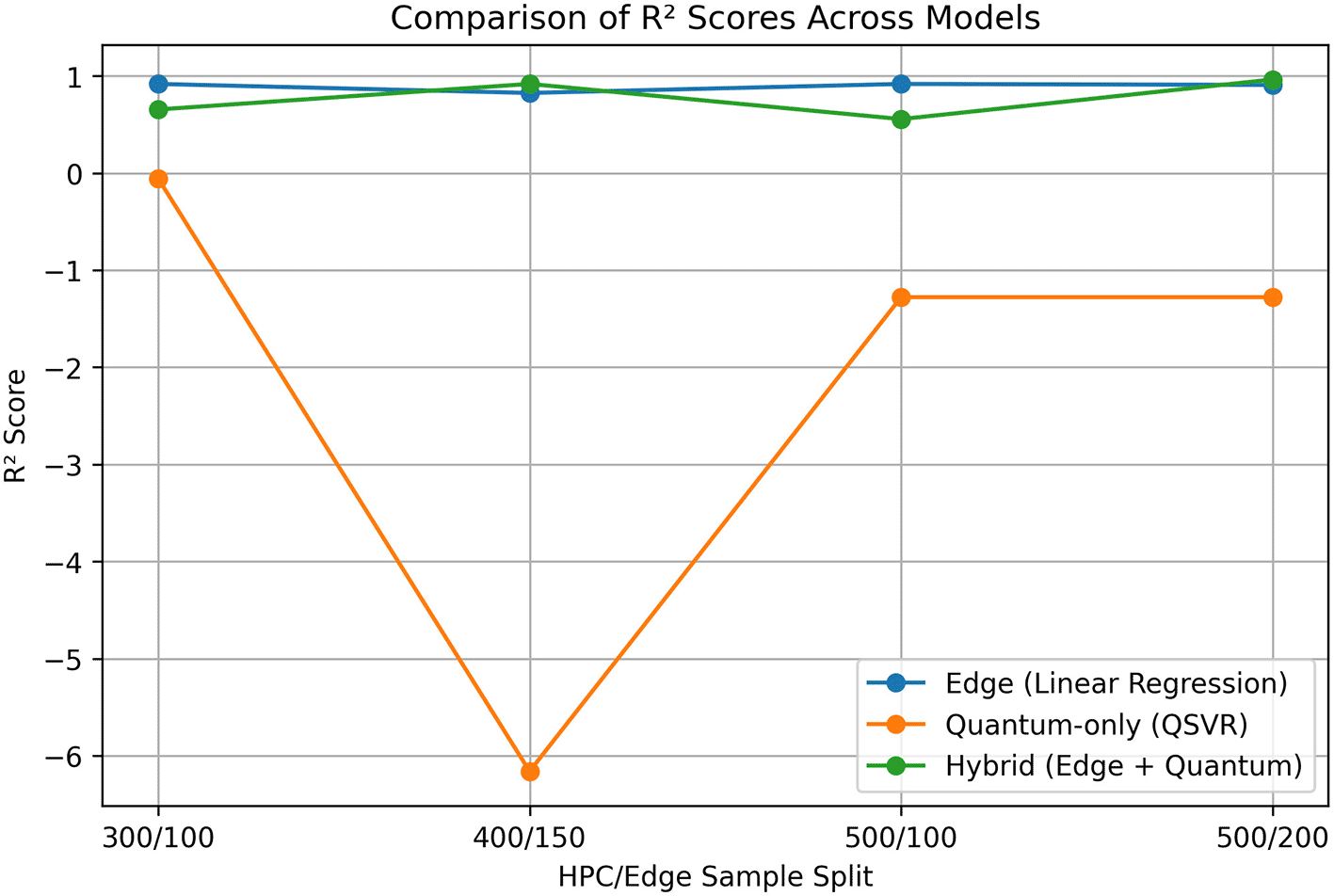
Figure 3. Comparison of
scores for Edge, Quantum-only, and Hybrid models across different HPC/Edge sample splits.
4.6 Summary of findings
Overall, the experimental analysis highlights the following key conclusions:
• The Edge model is effective for localized and low-latency forecasting, providing accurate predictions in linear regimes.
• The Quantum-only model struggles with data sparsity and instability, limiting its standalone effectiveness.
• The Hybrid model successfully integrates classical and quantum learning paradigms, achieving superior generalization and smoother forecast behaviour, especially when trained with an adequate balance of Edge and HPC data.
These results collectively demonstrate that the proposed hybrid quantum-classical framework enhances predictive performance and robustness, offering a promising direction for scalable quantum-assisted forecasting systems.







