Introduction
The three-dimensional (3D) organization of chromatin plays crucial roles in transcriptional regulation by facilitating or constraining interactions between cis-regulatory elements, such as enhancers and promoters (Furlong, Levine, 2018). Many models suggest that enhancer-promoter (E-P) communication is a key determinant of gene activation, often relying on chromatin loops to bring these elements into proximity (Schoenfelder, Fraser, 2019). However, the mechanisms underlying E-P communication (Chen et al., 2023; Kittle, Levo, 2025; Lim, Levine, 2021), and the extent to which E-P interactions vary between different cell types remains an open and highly debated question (Chen et al., 2023; Schaeffer, Nollmann, 2023). For instance, in Drosophila Melanogaster E-P contacts are pre-established and largely conserved across cell types during early embryonic development (Espinola et al., 2021; Ing-Simmons et al., 2021), but are dynamically reconfigured during later developmental stages as cell differentiation takes place (Pollex et al., 2024).
Ensemble sequencing-based approaches, such as Hi-C, have been extensively used to investigate chromatin architecture changes during differentiation, particularly in cultured cells (Bonev et al., 2017; Titus et al., 2024). More recently, high-resolution methods, such as capture Micro-C allowed the identification of specific chromatin loops between enhancers and promoters (Goel et al., 2023; Li et al., 2025). However, applying these approaches to study how 3D chromatin architecture changes between cell types in a complex tissue presents significant challenges. For instance, the need for large cell numbers is particularly challenging for cell types that are rare or difficult to isolate.
To overcome these limitations, several microscopy-based approaches have been developed to trace chromatin organization in single cells (Bintu et al., 2018; Cardozo Gizzi et al., 2019; Mateo et al., 2019). Among these, Hi-M combines sequential DNA fluorescence in situ hybridization (DNA-FISH) with other modalities (e.g. RNA or protein) to reconstruct chromatin conformation at kilo-base (kb) resolutions, and is therefore particularly well-suited for studying 3D genome folding in individual cells within complex tissues (Cardozo Gizzi et al., 2019; Espinola et al., 2021). By integrating cell-type markers, Hi-M allows the simultaneous detection of genome organization and cell identity, making it an ideal tool to investigate chromatin architecture changes in low-abundance cell populations (Messina et al., 2024). This capability is particularly relevant for the study of the Drosophila brain, where functionally distinct neuronal subtypes coexist in a highly structured environment.
The Drosophila brain provides an excellent model system to explore how chromatin conformation relates to neuronal function, learning, and memory (Aso et al., 2014). Despite extensive studies on its transcriptional landscape, the 3D chromatin organization of its neuronal subtypes remains largely uncharted. While a Hi-C/Micro-C dataset exists for the entire central nervous system (CNS) (Mohana et al., 2023), there is currently no cell-type-resolved chromatin structure available. Here, we address this gap by retrieving the 3D chromatin organization around a gene (rut) with specific expression in the mushroom body (MB) —a neuropil with critical roles in learning and memory (Zars et al., 2000). Using Hi-M, we provide five chromatin tracing datasets for the three major cell types of the MB: αβ -Kenyon cells (KC), α′β′-KCs, and γ-KCs, as well as for all KCs together, and for non-KC brain cells (
Table 1). These datasets will offer new insights into how 3D chromatin structure may contribute to neuronal identity and function.
Materials and methods
Fly lines
The transgene used in this study was UAS-nls-GFP (Bloomington stock #BL4770). All GAL4 driver lines utilized have previously been characterized (Aso et al., 2009), and include OK107-GAL4, which drives expression in all Kenyon cells (Connolly et al., 1996); c739-GAL4, targeting αβ Kenyon cells (Yang et al., 1995) ; c305a-GAL4, specific to α′β′ Kenyon cells (Krashes et al., 2007); and H24-GAL4, which labels γ Kenyon cells (Zars et al., 2000). These fly lines were a kind gift of J.M. Dura. All fly stocks and progeny from GAL4-UAS crosses were reared on standard cornmeal yeast extract medium at 25
°C. Genotypes and Bloomington catalogue numbers are provided in
Table 2.
Table 2. Fly lines used in this study.
| Name | Genotype | Bloomington stock |
|---|
| c739-GAL4 | y[1] w[67c23]; Pw[+mW.hs] = GawBHr39[c739] | 7362 |
| c305a-GAL4 | w[*]; Pw[+mW.hs] = GawBCka [c305a] | 30829 |
| H24-GAL4 | Pw[+mW.hs] = GawBH24 | 51632 |
| OK107-GAL4 | w[*]; Pw[+mW.hs] = GawBOK107 ey [OK107] | 854 |
| UAS-nls-GFP | w[1118]; Pw[+mC] = UAS-GFP.nls8 | 4776 |
Table 3. Raw Hi-M dataset statistics.
Replicate: number of biological replicates. N_ROIs: number of Regions of Interest. Unique traces: number of unique traces with more than two barcodes.
| File name | Cell type | Replicate | N_ROIs | Unique traces |
|---|
| traces_KCs_rep1.ecsv | All KCs | 1 | 9 | 3123 |
| traces_KCs_rep2.ecsv | All KCs | 2 | 10 | 5850 |
| traces_KC_AB_rep1.ecsv | αβ -KCs | 1 | 11 | 1795 |
| traces_KC_AB_rep2.ecsv | αβ -KCs | 2 | 15 | 4356 |
| traces_KC_ABp_rep1.ecsv | α′β′-KCs | 1 | 9 | 1101 |
| traces_KC_ABp_rep2.ecsv | α′β′-KCs | 2 | 17 | 1254 |
| traces_KC_ABp_rep3.ecsv | α′β′-KCs | 3 | 14 | 2755 |
| traces_KC_G_rep1.ecsv | γ-KCs | 1 | 11 | 908 |
| traces_KC_G_rep2.ecsv | γ-KCs | 2 | 6 | 475 |
| traces_KC_G_rep3.ecsv | γ-KCs | 3 | 21 | 5107 |
| traces_nonKC_rep1.ecsv | non-KCs
| 1 | 9 | 12014 |
| traces_nonKC_rep2.ecsv | non-KCs
| 2 | 10 | 17097 |
Drosophila brain dissection and cryo-sectioning
Adult female flies (2 to 5 days old) were collected from the previously cited fly lines following CO2 anesthesia. Flies were briefly dewaxed by immersing them in 70% ethanol for 2–5 seconds using forceps, then washed twice in 2× saline sodium citrate (SSC). Female flies were separately transferred into 2 mL Eppendorf tubes with a maximum of 15–20 flies per tube. Fixation and permeabilization were performed by incubating the flies in 4% paraformaldehyde (PFA) /0.5% PBT (1× phosphate-buffered saline (PBS) + 0.5% Triton X-100) on a rotating wheel for 3 hours at room temperature (RT). After fixation, the tubes were washed four times for 15 minutes each in 0.5% PBT, followed by two washes in PBS. During dissection, flies were kept in PBS on ice.
Drosophila brains were dissected on a Silgar polymer plate in ice-cold PBS, ensuring that brains dissected did not remain on the plate for more than 20 minutes to minimize potential brain damage. Dissected brains were post-fixed in 1.8 mL of 4% PFA, 0.5% PBT for 20 minutes, followed by three 20-minute washes in 0.5% PBT. All steps were performed on a rotating wheel at RT, and solutions were removed slowly to prevent brain resuspension. After the final wash, the remaining 0.5% PBT was carefully removed, leaving the brains in 200 μL of 0.5% PBT.
For cryoprotection, brains were incubated in a 30% filtered sucrose solution at 4
°C on a rotating wheel for 48 hours. 1 mL of solution was then removed from each 2 mL Eppendorf tube, and brains were gently resuspended and transferred onto a square cryomold (TED PELLA, cat. no. 27147-2). Next, the Optimal Cutting Temperature (OCT) embedding matrix was poured into the cryomold, which was then placed in a −80
°C freezer for storage. Samples were kept frozen for up to several months until cryosectioning.
Coverslips (Bioptechs, cat. no. 40-1313-0319) were cleaned with 70% ethanol and activated using air plasma for 30 seconds. Coverslips were then placed onto glass petri dishes and coated with 100 μL of 3-aminopropyltrimethoxysilane for 5 minutes at room temperature (RT). After incubation, slides were covered with deionized distilled water (ddH2O) for 10 minutes. Petri dishes were then transferred onto an orbital shaker and washed twice with ddH2O for 10 minutes each. Next, coverslips were incubated in a 0.5% glutaraldehyde/PBS solution for 30 minutes, followed by two washes with ddH2O. Once air-dried, slides were coated with a 20% poly-L-lysine solution (Sigma-Aldrich, cat. no. P8920) in PBS for 1 hour, then incubated overnight (O/N) in sterile ddH2O. The following day, slides were air-dried for 1–2 hours at RT.
Cryo-sectioning was performed using a cryostat, resulting in 10 μm thick slices that were carefully transferred onto silane-coated coverslips. Slides containing tissue sections were then air-dried for 1–2 hours at RT. For long-term storage, samples were first placed on ice for 15 minutes before being transferred to −20
°C.
Hi-M library design and amplification
Oligopaint libraries were designed as described previously (Cardozo Gizzi et al., 2019) and synthesized by CustomArray (Belgium). In this library, each barcode was encoded by 45 primary oligonucleotides, covering on average 3.2 kb. Each primary oligonucleotide consist of five distinct regions:
1. a 21 nt forward priming region for library amplification
2. two 20 nt probe-specific readout sequences
3. a 42 nt genome homology region
4. two 20 nt probe-specific readout sequences
5. a 21 nt reverse universal priming region
The forward and reverse priming sequences used were:
The procedure for oligopaint library amplification was as previously described (Cardozo Gizzi et al., 2019). Briefly, the protocol consists of seven steps:
1. Emulsion PCR (emPCR) to extract each library from the oligonucleotide pool using universal primers.
2. Limited-cycle PCR on the emPCR to identify the most efficient amplification cycle.
3. Large-scale PCR with a T7 promoter on the reverse primer.
4.
In vitro T7 transcription.
5. Reverse transcription to convert RNA into single-stranded DNA (ssDNA).
6. Alkaline hydrolysis to remove the intermediate RNA.
7. ssDNA purification and concentration.
Each barcode was sequentially hybridized within a microfluidics device (see next section) by using an imager oligo with a unique readout sequence. This imager oligo was labeled with an Alexa Fluor 647 fluorophore that is attached via a disulfide bridge, allowing chemical bleaching during sequential barcode imaging (Cardozo Gizzi et al., 2019). Adapters and fluorescently labeled imaging oligonucleotides were synthesized and purchased from Integrated DNA Technologies (IDT).
Hi-M labelling
Drosophila brain cryosections were removed from the -20
°C freezer and allowed to equilibrate at RT for 1 hour. Slides were then permeabilized in Sodium Citrate (10mM citrate, 0.05% Tween, pH 6.0), initially for 5 minutes at RT, followed by 25 minutes at 80
°C in a water bath. Slides were subsequently washed for 5 minutes with 2×SSC and incubated for 2 hours at RT in a wash buffer containing 50% formamide/2×SSC. Following incubation, slides were placed upside-down in a glass petri dish and sealed onto the Hi-M primary probe hybridization solution.
The hybridization solution contained 160–190 pmols of the primary Hi-M library diluted in 21 μL of FISH Hybridization Buffer (FHB), composed of:
Additionally, 1 μL of a 100 μM fiducial oligo solution was added to the hybridization mix. The fiducial library, used for drift correction during the pyHi-M analysis, includes sequences specifically designed to target satellites in Drosophila Melanogaster (Jagannathan et al., 2017; Li H et al., 2017a) with a complementary secondary probe bound to a non-cleavable Atto-488 fluorophore. Prior to the heat shock step, samples were incubated for 3 hours at 45
°C in a water bath. A heat shock was then applied for 5 minutes at 85
°C. Following this step, the petri dishes containing the samples were transferred to a humidified incubator and incubated overnight at 37
°C. The next day, cryosections were subjected to two consecutive washes with 50% wash buffer (WB) for 1 hour each. Samples were then sequentially washed using decreasing concentrations of WB as follows:
• 40% formamide for 40 minutes
• 30% formamide for 20 minutes
• 20% formamide for 20 minutes
• 10% formamide for 20 minutes
All wash steps were performed on an orbital shaker set to 50 rpm. After washing, slides were incubated for 20 minutes in 2× SSC, post-fixed in 4% paraformaldehyde (PFA) diluted in phosphate-buffered saline (PBS) for 10 minutes, and subsequently washed three times in 2× SSC. Finally, samples were stored at 4
°C in 2×SSC until further processing.The satellites sequences used were (Jagannathan et al., 2017; Li Q et al., 2017b):
• (AATAT)6: AATATAATATAATATAATATAATATAATAT
• (AACAC)7: AACACAACACAACACAACACAACACAACACAACAC
• X-359 bp: TTTTCCAAATTTCGGTCATCAAATAATCAT
• (AATAC)6: AATACAATACAATACAATACAATACAATAC
• (AAGAG)6: AAGAGAAGAGAAGAGAAGAGAAGAGAAGAG
• (AATAACATAG)3: AATAACATAGAATAACATAGAATAACATAG
Immunostaining for GFP detection in Kenyon cells
DNA-FISH labeling results in loss of GFP fluorescence; therefore, an immunostaining protocol against GFP was employed to detect Kenyon cells. Slides were first incubated for 2 hours in 0.1% bovine serum albumin (BSA) in 0.1% PBT (1×PBS + 0.1% Triton X-100). A chicken GFP polyclonal antibody (anti-GFP) was diluted 1:200 (Invitrogen, catalogue no. A10262) in 0.1% BSA-PBT and incubated overnight at 4
°C in a humid chamber. The next day, brain cryosections were washed three times for 20 minutes in PBT. Samples were then incubated at room temperature with a 1:500 dilution of goat anti-chicken secondary antibody (Invitrogen, catalogue no. A21449) in PBT for 3 hours. Following antibody hybridization, three additional PBT washes of 10 minutes each were performed. To remove residual Triton X-100, samples were washed rapidly twice with PBS. Slides were post-fixed for 5 minutes in 4% PFA diluted in PBS, followed by three additional PBS washes. Finally, samples were stored in 2× SSC at 4
°C until imaging.
Hi-M acquisition
Hi-M experiments were conducted using a custom-built widefield epifluorescence microscope as described previously (Fiche et al., 2024) (Fig. 1A). The setup included a Rapid Automated Modular Microscope (RAMM) (Applied Scientific Instrumentation, Oregon, US) coupled with a microfluidic device, as previously described in (Barho et al., 2022). The microscope and fluidics system were controlled via Qudi-HiM, a custom hardware control package (Barho et al., 2022). The fluidics system enabled automated and sequential probe hybridizations, with solutions delivered to the sample using a combination of three eight-way valves (HVXM 8-5, Hamilton), a negative pressure pump (MFCS-EZ, Fluigent), and an FCS2 flow chamber (Bioptechs, cat. no. 03060319-2-NH). Fluorescence excitation was achieved using three different lasers: 405 nm (Obis 405, 100 mW, Coherent), 488 nm (Obis 488, 100mW, Coherent), and 642 nm (VFL-0-1000-642-OEM1, 1W, MPB Communications Inc.). Fluorescence was collected through a Nikon APO x60 1.2 NA water immersion objective lens mounted on a closed-loop piezoelectric stage (Nano-F100, Mad City Labs Inc.). Image acquisition was performed using an sCMOS camera (ORCA Flash 4.0 V3, Hamamatsu) with an effective optical pixel size of 106 nm. 3D stacks were performed with a z-spacing of 250 nm. To correct axial drift in real time, a custom-built autofocus system was employed, consisting of a 785 nm laser (OBIS 785, 100 mW, Coherent) and an infrared-sensitive laser position sensor (OBP-A-4L, Newport).
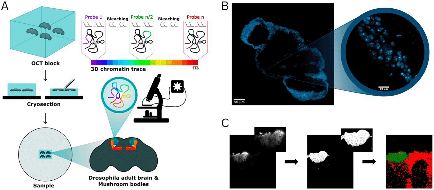
Figure 1. (A) Schematic representation of the pipeline for sample preparation and imaging using Hi-M.
Each color in the 3D chromatin trace colorbar represents a barcode of 3 kb in size. (B) Representative image of a Drosophila brain cryosection. Nuclei are shown in blue (DAPI), the fluorescence signal emitted by a single DNA-FISH barcode of 3 kb are shown in red (Alexa Fluor 647). Magnifications: 20x (left), 60x (right). (C) Procedure used to assign chromatin traces to specific cell types. Representative image of the anti-GFP staining against Kenyon cells (from a OK107-GAL4 x UAS-nls-GFP cross) (left panel), anti-GFP signal segmented with ilastik (middle panel), assignment of localizations to Kenyon cells (green) and non-Kenyon cells (red).
The slide containing Drosophila brain cryosections was mounted on the fluidics device (FCS2 chamber, Bioptechs) and incubated with the fiducial library imager (25 nM Atto-488, 2×SSC, 40% v/v formamide) for 20 minutes, followed by a 10-minute wash with washing buffer (WB) solution (2×SSC, 40% v/v formamide). After a 5-minute wash with 2×SSC, nuclei were stained with 0.5–1 μg/mL DAPI in PBS for 20 minutes. Imaging buffer (IB) (1× PBS, 5% glucose, 0.5 mg/mL glucose oxidase, and 0.05 mg/mL catalase) was used to minimize fiducial photobleaching during acquisition. An image stack was acquired for each of the 10–20 regions of interest (ROIs), each measuring 217 μm × 217 μm and containing a single Drosophila brain. The DAPI, fiducial, and GFP immunostaining signals were sequentially imaged using 405 nm, 488 nm, and 647 nm lasers, respectively, with a z-step size of 250 nm over a total range of 17.5 μm. Next, readout probes were sequentially hybridized, imaged, and photobleached to image all the barcodes in the Hi-M library (see example in Fig. 1B).The following steps were repeated for each of the 25 probes:
1. Injection and incubation of readout probes (40 nM secondary probe in WB) for 10 minutes.
2. Wash with WB solution for 10 minutes.
3. Injection of IB and sequential acquisition of fiducial and probe signals using 488 nm and 641 nm lasers.
4. Chemical bleaching of the imaging probe with 2× SSC containing 50 mM tris(2-carboxyethyl) phosphine (TCEP, Sigma-Aldrich, cat. no. 646547).
5. Final wash with 2× SSC for 10 minutes before the next hybridization cycle.
At the end of the experiment, an AF647-labeled imager oligo with a sequence complementary to the reverse primer of the Hi-M library was used to label all the oligonucleotides in the library at once. This probe-finding image was sub-sequentially used to perform chromatin tracing (see below).
Hi-M analysis
Raw TIFF images were deconvolved using Huygens Professional 21.04 (Scientific Volume Imaging, https://svi.nl). Hi-M analysis was performed using pyHi-M, a homemade analysis pipeline (Devos et al., 2024). For each cycle of hybridization, fiducial images were used to register the corresponding barcode and probe-finding images using global and local registration methods (Devos et al., 2024). Next, barcode and probe-finding images were segmented in 3D using a neural network, followed by 3D localization of the center of each barcode mask using 3D Gaussian fitting (Devos et al., 2024). Finally, chromatin traces were built by combining the DNA-FISH spots colocalizing within single probe-finding masks. Only traces containing at least two barcodes were kept. Barcodes duplicated in a trace were removed from that trace.
After final outputs of pyHiM were generated, the anti-GFP signal was segmented using ilastik (Berg et al., 2019) (a machine learning toolkit for segmentation) and a homemade software to assign each trace to either the cell type of interest or the other cells of the brains (Fig. 1C).
Median PWD matrices were obtained by calculating the median of the distribution for each barcode combination. Hi-M proximity frequencies were calculated using standard procedures (Cardozo Gizzi et al., 2019; Espinola et al., 2021) that estimate the number of chromatin traces in which PWDs were smaller than a pre-defined cut-off distance threshold, normalized by the total number of observations in the distribution. A standard cut-off distance threshold of < 150 nm was used (Mateo et al., 2019; Messina et al., 2023). Hi-M proximity frequency maps were obtained by performing this operation for all combinations of barcodes (e.g. Fig. 2B).
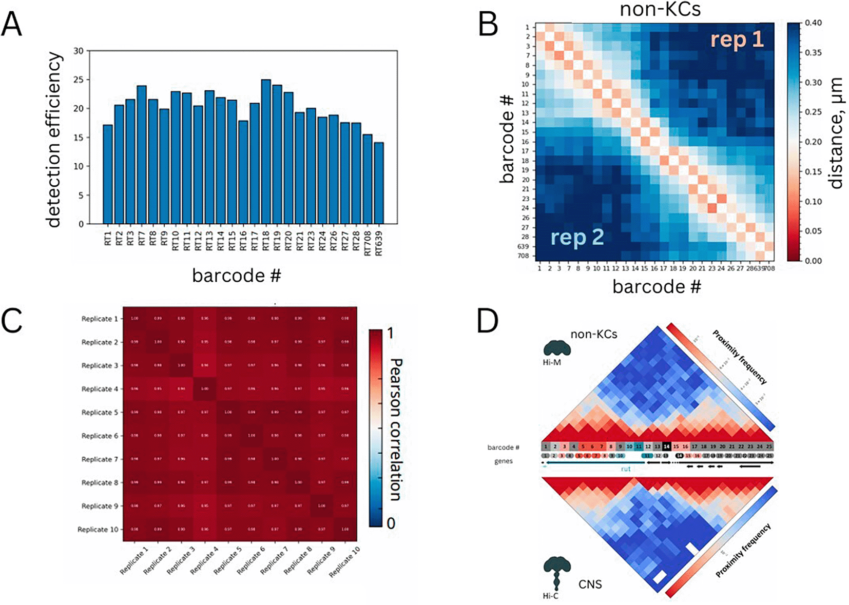
Figure 2. (A) Efficiency of detection for each barcode.
(B) Median pairwise distance map for non-Kenyon cells. Two different replicates are shown on the top right and bottom left matrices. (C) Pearson correlations between pairs of replicates.
(D) Comparison between Hi-M proximity frequencies in non-KCs and interpolated Hi-C normalized counts for the same genomic region in the adult Drosophila central nervous system (CNS) from Mohana et al. (
Mohana et al., 2023). Hi-M barcodes were colored as follows: promoter (teal); enhancers (red, pink); accessible regions (light gray); inaccessible regions (dark gray). Genes are represented with the following color code: rut (dark teal), other genes (black).
We estimated the standard error of the median PWD by performing bootstrapping analysis. For each barcode combination, we resampled the distribution of single-allele PWD distances 1000 times and computed the median for each resampled dataset. Finally, we calculated the standard deviation of these medians to estimate the standard error of the mean for each barcode combination, which was represented as a map (e.g. Fig. 4C).
PWD distribution analysis
Spatial proximity distributions between loci were modeled using a bimodal two-state Gaussian model previously described in (Remini et al., 2024). The observed distribution of pairwise distances (PWDs) between genomic segments i and j, denoted by Pi j(r), was fitted by a linear combination of two Gaussian distributions representing bound (B) and unbound (U) chromatin states:
(1)
where
fB and 1
− fU are the fractions of barcode-barcode pairs existing in the bound (B) and unbound (U) states, respectively. The Maxwell distribution
g(
r;
R) for distance
r and characteristic radius
R is defined as:
(2)
To ensure stability of the fits, we imposed specific constraints on the characteristic radii of each state: the Bound state (RB) was constrained to be less than 200 nm, and the Unbound state (RU) was constrained to be greater than 200 nm. These thresholds were chosen based on previous experimental and theoretical considerations. Parameters of the model, including the fraction of Bound state (fB) and the radii (RB, RU), were determined through maximum likelihood estimation, and uncertainties on each parameter were obtained from the covariance matrix of the fits. The quality of the fits was assessed using the Pearson’s chi-square
test.
Datasets technical validation
Labeling efficiency
For each acquisition, we verified that DNA-FISH spots corresponding to both barcodes and loci masks appeared as diffraction- limited spots (Fig. 1B). Next, we estimated the detection efficiency of each barcode by calculating the frequency with which loci masks were occupied by at least one DNA-FISH spot of the corresponding barcode (Mateo et al., 2019). This calculation was repeated for all barcodes and is represented in Fig. 2A, showing that detection efficiencies exceeded 60%, typical of chromatin tracing datasets at this genomic resolution (i.e. 3 kb) (Cardozo Gizzi et al., 2019; Espinola et al., 2021; Mateo et al., 2019).
Comparison between replicates
In this study, we performed at least two independent biological replicates per cell type. Comparisons between replicates were conducted by representing the median pairwise distance (PWD) maps, which are obtained by calculating the median PWD for each combination of barcodes. For non-KCs, PWD maps from different replicates were highly similar (Fig. 2C). Additionally, we quantified this similarity by calculating the Pearson correlation coefficient between median PWDs across replicates (Fig. 2C). For non-KCs, Pearson correlation coefficients between any combination of replicates were consistently above 0.9.
These comparisons were also performed for the remaining datasets: (1) all KCs grouped together (Figs. 3A-B), (2) γ-KCs (Figs. 4A-C), (3) α′β′-KCs (Figs. 5A-C), and (4) αβ -KCs (Figs. 6A-B). In all cases, the PWD maps of the replicates were highly similar and exhibited high Pearson correlation coefficients, providing additional validation of the results.
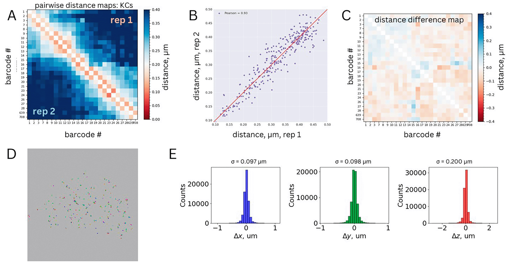
Figure 3. (A) Median pairwise distance map for Kenyon cells.
Two different replicates are shown on the top right and bottom left matrices. (B) Correlation between the median pairwise distances measured for the two replicates. Pearson correlation coefficient is shown as legend. (C) Standard deviation matrix for the merged dataset obtained from bootstrapping analysis. (D) Representative chromatin traces from a single ROI, xy projection. Each barcode is represented by a different color. Barcodes belonging to the same trace are linked by a black line. (E) Physical distance distributions between first genomic neighbors for each dimension (xyz).
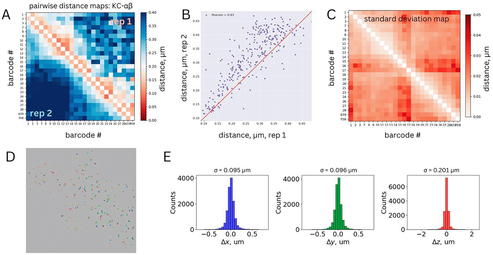
Figure 4. (A) Median pairwise distance maps for αβ Kenyon cells.
Two different replicates are shown on the top right and bottom left matrices. (B) Correlation between the median pairwise distances measured for the two replicates. Pearson correlation coefficient is shown as legend (R = 0.83). (C) Standard deviation matrix for the merged dataset obtained from bootstrapping analysis. (D) Representative chromatin traces from a single ROI, xy projection. Each barcode is represented by a different color. Barcodes belonging to the same trace are linked by a black line. (E) Physical distance distributions between first genomic neighbors for each dimension (xyz).
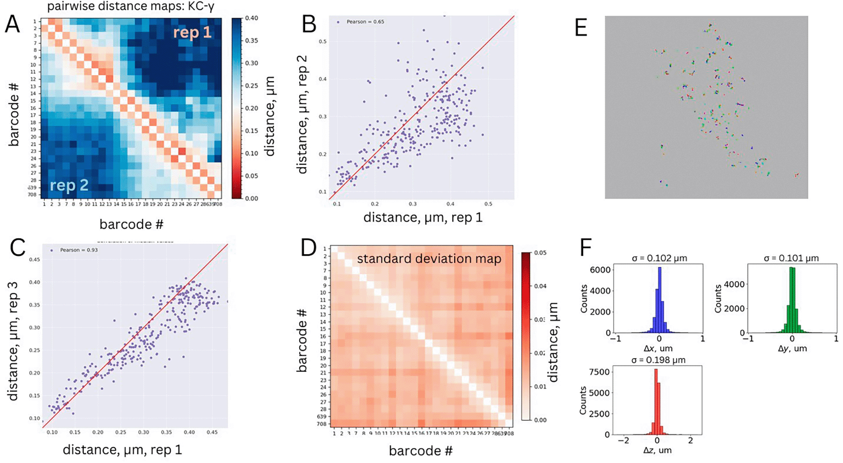
Figure 5. (A) Median pairwise distance map for γ Kenyon cells.
Two different replicates are shown on the top right and bottom left matrices. (B-C) Correlation between the median pairwise distances between replicate 1 and replicates 2 (panel B) or 3 (panel C). Pearson correlation coefficients are shown in legends. (D) Standard deviation matrix for the merged dataset obtained from bootstrapping analysis. (E) Representative chromatin traces from a single ROI, xy projection. Each barcode is represented by a different color. Barcodes belonging to the same trace are linked by a black line. (F) Physical distance distributions between first genomic neighbors for each dimension (xyz).
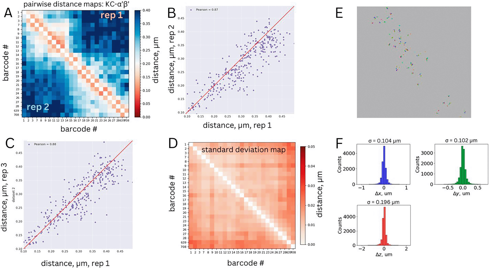
Figure 6. (A) Median pairwise distance map for α′β′ Kenyon cells.
Two different replicates are shown on the top right and bottom left matrices. (B-C) Correlation between the median pairwise distances between replicate 1 and replicates 2 (panel B) or 3 (panel C). Pearson correlation coefficients are shown in legends. (D) Standard deviation matrix for the merged dataset obtained from bootstrapping analysis. (E) Representative chromatin traces from a single ROI, xy projection. Each barcode is represented by a different color. Barcodes belonging to the same trace are linked by a black line. (F) Physical distance distributions between first genomic neighbors for each dimension (xyz).
Comparison to existing Hi-C dataset
To further validate these results, we compared the Hi-M proximity frequency map (see Methods) for non-KCs, which represent the majority of cells in the adult fly brain (~95.000 out of 100.000), to a publicly-available Hi-C dataset for the adult Drosophila central nervous system (Mohana et al., 2023). The Hi-M and Hi-C maps were remarkably similar, despite profound differences between the two methodologies. This comparison provides further validation for our datasets (Fig. 2D). We note that this comparison can only be performed for non-KCs (representing the vast majority of cells in the fly brain) as Hi-C datasets for Drosophila brain cell types are not available.
Bootstrapping analysis
PWD maps provide a reliable estimation of the mean distance between any combination of barcodes. However, they do not capture the variation within a population of single alleles. To assess this variation, we performed a bootstrapping analysis on the merged datasets (see Methods section, Hi-M analysis). For all analyzed cell types, the standard errors of the mean were below 50 nm (Figs. 3C, 4D, 5D, 6C). These quantitative validations confirm that the precision of our mean PWD distance measurements was 50 nm or better, further validating the accuracy of the dataset.
Physical distributions between first neighbors
Because of the polymeric nature of chromatin, genomically close barcodes tend to be spatially proximal in 3D space (Cardozo Gizzi et al., 2019). In our Hi-M library design, adjacent barcodes are separated by an average genomic distance of 3 kb. At this scale, we expect their physical separation to be approximately
~100−200 nm (Cardozo Gizzi et al., 2019; Mateo et al., 2019). We used this criterion as an additional validation of chromatin tracing accuracy in our datasets (Figs. 3D, 4E, 5E, and 6D). To this end, we computed the 3D distances between genomically-adjacent barcodes for each chromatin trace and plotted their distributions for each dataset. We expect these distributions to be centered at zero and with a standard deviation between 57 and 110 nm (estimated from the mean distance as
/
). The measured standard deviations are within the anticipated range (Figs. 3E, 4F, 5F, and 6E).
Ethics and consent
Ethical approval and consent were not required.