1 Introduction
The Internet of Things (IoT) now interconnects billions of resource-constrained devices across smart homes, industrial control systems, healthcare, and critical infrastructure, greatly enlarging the network attack surface. Weakly secured endpoints are routinely conscripted into large-scale botnets. The Mirai outbreak alone marshalled hundreds of thousands of IoT devices into record-setting distributed denial-of-service (DDoS) campaigns, and its many variants continue to dominate the IoT threat landscape.1,2 As attack volume and diversity grow, network intrusion detection systems (IDSs) remain an indispensable line of defence, complementing firewalls and access control by inspecting traffic for malicious behaviour.3,4
In modern IoT deployments, detection is increasingly pushed to the network edge, onto gateways and aggregation nodes close to the data sources, so that threats can be flagged with low latency and without exporting sensitive traffic to the cloud. Edge operation, however, imposes severe constraints, since the detector must sustain high, bursty packet rates at or near line rate while fitting within tight CPU, memory, and energy budgets.4,5 These constraints sit in direct tension with the dominant trend in IDS research, where deep learning models such as multilayer perceptrons, convolutional and recurrent networks, and attention-based architectures deliver state-of-the-art detection on recent flow-level benchmarks.6–8 Such models are frequently too heavy for constrained gateways, forcing practitioners into an unfavourable accuracy, latency, and footprint trade-off.
A large body of work narrows this gap by making a single model cheaper. Static compression, namely pruning, quantization, and knowledge distillation, reduces parameter count and arithmetic cost,9–12 while feature selection and dimensionality reduction shrink the input and, implicitly, the model.5,13 These techniques lower the average cost but apply the same fixed computation to every flow, regardless of how hard each flow is to classify. Yet network traffic is highly skewed in difficulty. The overwhelming majority of flows are easily separable, and only a small minority sit near decision boundaries or reflect rare, novel, or evasive behaviour that genuinely warrants full-capacity inference.14 Spending identical compute on trivial and difficult flows alike is therefore wasteful at the edge.
This observation motivates conditional (input-adaptive) computation, in which the amount of computation varies per input.15,16 Representative mechanisms include early-exit and cascade architectures that terminate easy inputs in shallow stages,17,18 and sparsely gated mixtures that route each input to a subset of experts.19 In security analytics, the same principle appears as staged or multi-level pipelines that filter obviously benign traffic with cheap models before invoking expensive analysis.20–22 Across these systems, however, the routing decision, that is, when to escalate an input to a more capable model, is typically made by a hand-tuned confidence threshold or an ad-hoc rule, and the choice of routing signal is rarely studied in its own right. It remains unclear which signal best identifies the flows that truly need heavy computation, how its operating threshold should be selected without leaking test information, how close such routing can come to an ideal oracle, and whether a routing policy tuned on one network transfers to another.
A recent conference paper23 instantiated conditional computation for tabular IoT IDS as a dual-path
detector. In that design, features are standardized and projected onto a low-dimensional subspace obtained by principal component analysis (PCA), and a tiny multilayer perceptron (MLP) on the latent space produces a fast prediction together with a maximum-softmax-probability (MSP) confidence; flows with
are accepted on the tiny path, and the remainder are escalated to a heavy full-feature MLP. That work established the architecture and showed that escalating only a small fraction of flows recovers most of the heavy model’s accuracy. Yet it treated the gate as a fixed MSP threshold and left open the questions that determine whether such a design is trustworthy in deployment. These are which signal should drive escalation, how to set its threshold safely, how far escalation can be pushed before it stops helping, and whether the resulting policy generalizes across heterogeneous networks.
This paper turns the dual-path idea into a systematic study of the escalation gate. We evaluate a broad family of routing signals against a learned router and an oracle upper bound, add calibration and a leakage-free thresholding rule, probe the ceiling of confidence-based routing, and assess robustness, cost, significance, and cross-dataset transfer. We conduct the study on three public IoT/network intrusion-detection benchmarks, namely ACI-IoT-2023,24 TabularIoTAttacks-2024,7 and the large, long-tailed CICIoT2023,25 in both multi-class and binary settings, over multiple random seeds, with statistical significance testing throughout.
Contributions
We make five main contributions.
1.
A unified routing-signal family. We benchmark MSP, entropy, margin, energy, temperature-scaled confidence, and latent norm against a learned router and an oracle bound, all at matched escalation cost (Sec. 5.2).
2.
Calibration-aware, leakage-free thresholding. We add temperature scaling and a validation-only rule for choosing the escalation budget, and report the selection gap (Sec. 5.3, 5.4).
3.
An oracle gap and its mechanism. On CICIoT2023, routing cannot reach the heavy model because the tiny model is confidently wrong on a few high-volume attack families, which are therefore never escalated; no cheap routing signal we test, confidence-based or confidence-independent, closes it (Sec. 5.6).
4.
An honest ensemble ablation. Deep-ensemble and disagreement-based signals give only marginal gains and are not cost-effective at these sizes (Sec. 5.7).
5.
Deployment-facing evaluation. We assess group-dropout robustness, latency and model size, McNemar significance, and cross-dataset transfer (Sec. 5.8–5.11).
Beyond the conference version,23 this article adds a third, substantially harder benchmark (CICIoT2023, used here with 27 classes after a rare-class floor), the entire routing-signal study, calibration and cost-optimal thresholding, the oracle-gap analysis, the ensemble ablation, and the robustness, significance, and cross-dataset experiments.
Organization
Section 2 reviews lightweight and conditional-compute IDS and uncertainty estimation. Section 3 formalizes the dual-path detector, the routing-signal family, the learned router, calibration, and cost-optimal thresholding. Section 4 describes the datasets, models, and protocol. Section 5 presents the results (E1–E9), Section 6 discusses implications and deployment guidance, Section 7 states limitations, and Section 8 concludes.
2 Background and related work
We review prior work on deep learning for IoT intrusion detection, lightweight and compressed models, conditional computation, and uncertainty estimation, then position our contribution against it.
2.1 Deep learning for IoT intrusion detection
IoT networks face a fast-evolving threat landscape, from reconnaissance scans to volumetric floods launched by botnets such as Mirai.1,2 Recent surveys document a rapid shift from classical classifiers to deep models for flow-based detection.3,4,6,26 On tabular benchmarks such as ACI-IoT-202324 and CICIoT2023,25 MLP, convolutional (CNN), recurrent, and attention-based models reach strong accuracy,7,8 and resilience to adversarial traffic pushes capacity higher still.14 This accuracy carries inference and memory costs that are hard to sustain at the edge.
2.2 Lightweight and compressed detection models
One direction makes a single model cheaper. Pruning, quantization, and knowledge distillation cut size and cost with limited accuracy loss,9–11 and recent IDS work distills compact detectors for IoT and unmanned aerial vehicle (UAV) gateways.12,27 A complementary direction shrinks the input through feature selection or dimensionality reduction such as PCA and autoencoders.5,13 These methods lower the average cost but apply the same fixed computation to every flow.
2.3 Conditional and adaptive computation
A second direction varies computation per input,15,16 through early-exit networks17,18 and sparsely gated mixtures of experts.19 In security analytics the same idea appears as two-stage pipelines20,21 and as confidence-driven offloading that escalates uncertain inputs to a stronger model or node.22,28,29 Across these systems the escalation decision is usually a fixed threshold or a hand-crafted rule, and the choice of routing signal is rarely studied in its own right.
2.4 Uncertainty estimation and calibration
Routing is at heart a question of predictive uncertainty. MSP is the standard error and out-of-distribution baseline,30 with entropy, margin, and energy scores31 as alternatives, and temperature scaling as a simple calibration step.32 Epistemic uncertainty is estimated by deep ensembles,33 Monte-Carlo dropout,34 and Bayesian Active Learning by Disagreement (BALD),35 while committee disagreement is classical in active learning.36 A closely related line is selective prediction and failure detection, which abstains on or flags likely-wrong inputs using confidence37,38; a known limitation there, which we meet again below, is that a model’s own softmax cannot expose its confident errors. These signals are typically used for abstention, out-of-distribution detection, or data acquisition rather than for cheap-to-heavy routing inside an IDS.
2.5 Positioning of this work
Building on the dual-path detector of,23 we treat the escalation gate as the object of study rather than a fixed threshold. We compare the uncertainty measures above as routing signals against a learned router and an oracle reference, and analyze calibration, cost-optimal thresholding, the performance ceiling, robustness, and cross-dataset transfer over three benchmarks. To our knowledge this is the first systematic comparison of routing signals for conditional-compute intrusion detection on tabular IoT traffic.
Table 1 positions the work against representative conditional-compute and IDS systems.
Table 1. Positioning against representative adaptive-compute and IDS work.
“Signal studied” marks whether the choice of routing/escalation signal is itself analysed rather than fixed a priori.
| Approach | Per-input
| Signal studied | IoT IDS |
#IDS datasets |
|---|
| Early-exit/cascade17,18 | yes | no | no | – |
| Mixture-of-experts19 | yes | no | no | – |
| Two-stage IDS20,21 | yes | no | yes | 1 |
| Offloading IDS22,28,29 | yes | no | yes | 1–2 |
| Dual-path (conf.)23 | yes | partial | yes | 2 |
| This work
| yes | yes
| yes | 3
|
3 Methods
This section formalizes the dual-path detector and the gate that routes each flow between its two paths. After fixing notation and the data pipeline, we define the two paths and the decision rule, then the routing signals, the learned router, calibration, threshold selection, the ensemble variant, and the oracle bound.
3.1 Problem formulation and notation
We treat intrusion detection as supervised classification of network flows. A flow is a feature vector
with label
, where
. In the multi-class setting each class is benign traffic or a specific attack family, and in the binary setting all attacks are merged into a single positive class. Given a labelled set
, our goal is not a single classifier but a two-model system that approaches the accuracy of a large model at close to the cost of a small one, by sending only the difficult flows to the large model. Throughout,
denotes standardized features,
the latent code,
the tiny-model posterior,
its logits, and
a predicted label.
3.2 Datasets and preprocessing
Table 2 summarizes the three public benchmarks we evaluate on, namely ACI-IoT-2023,24 TabularIoTAttacks-2024,7 and CICIoT2023.25 CICIoT2023 has a long-tailed label distribution, so we drop classes with fewer than
samples (7 of 34), leaving 27 classes so that stratified splits are well defined.
Table 2. Datasets.
Rows after cleaning; CICIoT2023 after the rare-class floor.
| Dataset | #flows | #feat. | #classes |
benign label |
|---|
| ACI-IoT-2023 | 1,048,575 | 83 | 11 | Benign |
| TabularIoTAttacks-2024 | 722,144 | 84 | 12 | (benign traffic) |
| CICIoT2023 | 1,047,996 | 46 | 27 | BenignTraffic |
Non-label columns are cast to numeric, infinities are mapped to missing values, missing values are imputed with training-set medians, and features are clipped to
. We use a stratified
train/validation/test split. Each feature is then standardized with statistics from the training split,
where
and
are the per-feature training mean and standard deviation and
is elementwise division. The scaler, and any PCA basis, are fit on the training split only and applied unchanged to validation and test. All experiments use seeds.
423.3 Dual-path detector
Figure 1 gives an overview. Every flow runs the cheap tiny path on an edge gateway; only the flows the gate marks as uncertain are escalated to the heavy path, which may run on the same node or on a more capable near-edge or cloud resource.
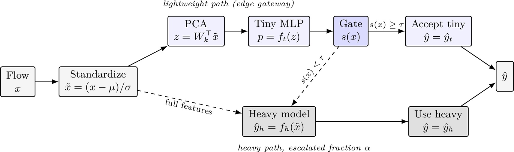
Figure 1. The dual-path detector.
Standardized features feed a lightweight path (PCA then a tiny MLP) that produces a prediction and a gate score
. Confident flows (
) are answered by the tiny path on the edge gateway; uncertain flows are escalated to a heavy full-feature model. Under a budget, the top-
fraction by
is escalated instead of using a fixed
.
The heavy path is a full-feature MLP with two hidden layers that outputs a posterior
. The tiny path first compresses the standardized features to
principal components and then applies a single-hidden-layer MLP,
where
holds the top-
PCA directions (
retains
of the variance on ACI-IoT-2023 and TabularIoTAttacks-2024) and the tiny hidden layer has
units. We use a linear projection because it retains most of the variance at negligible cost and keeps the tiny path cheap; a non-linear autoencoder latent is a natural alternative that we do not pursue here, since our focus is the gate rather than the compressor. The two paths give predictions
and
. A gate routes each flow to exactly one path,
where a flow is escalated when its routing score
(Sec. 3.4) lies in the top-
fraction under a fixed budget, or exceeds a threshold
. Since the tiny path runs on every flow and the heavy path only on the escalated fraction
, a simple approximation of the average classifier inference time is
and we also measure the true end-to-end latency, including preprocessing, in Sec. 5.9. Algorithm 1 summarizes inference for one flow.
Algorithm 1. Dual-path inference for a flow
x
(threshold mode).
Require: scaler
; PCA basis
; tiny
; heavy
; gate score
; threshold
.
1.
(standardize)
2.
;
;
(tiny path, always run)
3. compute routing score
from
,
(or the learned router)
4.
if
then
(escalate to heavy path)
5.
else
6.
return
In budget mode, the scores
of a batch are ranked and the top-
fraction is escalated, which fixes the heavy cost regardless of the score’s scale.
3.4 Routing-signal family
A gate is fully determined by its routing score
, where a higher value marks a flow as more in need of the heavy path. We study six scores derived from the tiny posterior
, its logits
, and the latent code
,
where
and
are the two largest posterior entries and
is the calibration temperature of Sec. 3.6. Casting every gate as a score that we rank and threshold places all of them, including a random baseline and the latent-norm baseline, on an identical cost footing and lets us compare them at a matched escalation fraction
.
3.5 Learned router
Rather than trusting a single hand-chosen score, we learn one. Let
stack the scalar signals above with the latent code
. A small MLP router
is trained on the validation split to predict whether the tiny model is about to err, and at test time its predicted error probability is used as the routing score,
Training the router on the validation split, rather than on the data the tiny model already fit, prevents it from inheriting the tiny model’s training-time optimism.
3.6 Confidence calibration
Because several gates compare confidences across flows, miscalibration distorts routing. We apply temperature scaling, fitting a single scalar
on the validation set
by minimizing the negative log-likelihood,
and we report the Expected Calibration Error (ECE) over
equal-width confidence bins,
where
and
are the accuracy and mean confidence of the flows whose top probability falls in bin
.
3.7 Cost-optimal, leakage-free threshold selection
Rather than hand-setting the operating point, we select the escalation budget on the validation split. Let
be the validation F1-macro of the dual system at budget
, and let
and
be the tiny-only and heavy-only validation scores. We pick the smallest budget that recovers a fraction
of the gap between them,
with
in our experiments. We then freeze
and report test performance, and we measure selection leakage as the difference between this frozen point and the best test point at the same budget.
3.8 Ensemble-disagreement signals
As an epistemic alternative to single-model confidence, we train a tiny ensemble of
MLPs that share the latent representation but differ in random seed, giving member posteriors
, member predictions
, and an ensemble mean
. From these we form
together with the variation ratio, the ensemble entropy
, and the ensemble-averaged confidence
. The ensemble mean
also serves as a more accurate tiny prediction. These signals capture model uncertainty that a single softmax cannot express.
3.9 Oracle bound
To bound what any gate can achieve at a given budget, we include an oracle score
which escalates exactly the flows the tiny model would misclassify. The oracle is not deployable, since it uses the true label, but it upper-bounds the F1 of every routing signal and reveals how much of the heavy-tiny gap is in principle recoverable by routing.
4 Experimental setup
This section describes the models and baselines, the evaluation protocol and metrics, the statistical test, and how we measure runtime, so that every result in Sec. 5 can be reproduced.
4.1 Models and training
All neural models are scikit-learn MLPClassifier networks trained with Adam, a batch size of
, and
epochs. The heavy path uses two hidden layers of sizes
on the full standardized features, and the tiny path uses a single hidden layer of
units on the PCA-
latent code. We also vary the latent dimension over
to study its effect. The learned router of Sec. 3.5 is a small MLP with one hidden layer of
units trained on the validation split, and the ensemble of Sec. 3.8 uses
tiny networks that differ only in random seed.
4.2 Baselines
For context we add three classical lightweight baselines on the same PCA-
features, namely multinomial logistic regression, a random forest with
trees of depth
, and a tiny MLP trained on the
highest-variance raw features. The standalone heavy and tiny models, together with the oracle gate of Sec. 3.9, bound the achievable range at each operating point.
4.3 Evaluation protocol and metrics
We report test accuracy and macro-averaged F1, the latter being our primary metric because the datasets are highly imbalanced. Gate comparisons are made at a matched heavy fraction so that all routing signals incur identical cost, and the main operating point escalates
of flows unless stated otherwise. We use
as a representative low budget; the full accuracy-cost curves in Sec. 5.2 sweep the budget continuously and show the trends are monotone rather than specific to this choice. Robustness is evaluated under random
feature dropout and under coherent feature-group dropout that zeros about
of the features in eight correlated groups, and calibration is measured by the ECE with
bins. Every configuration is run over three seeds (
,
,
), and we report the mean.
4.4 Statistical testing
To check whether differences between gates are real rather than sampling noise, we use McNemar’s test39 on the shared test set, which is the appropriate paired test for two classifiers evaluated on the same examples. We report the resulting
-values alongside the F1 differences.
4.5 Implementation and runtime measurement
All experiments run on a single CPU-only workstation. Inference time is averaged over five repetitions, and we report both the classifier-only time of Eq. (4) and the true end-to-end latency that includes standardization, PCA projection, the routing decision, and the heavy pass on escalated flows. Model size is the serialized footprint of each network. Because absolute timings are hardware-dependent, we emphasize relative comparisons and serialized sizes. The full code and the per-experiment result tables are released for reproducibility.
5 Results
We present the results in three parts. The first confirms reproduction and characterizes the standalone heavy and tiny models (Sec. 5.1). The second makes the routing gate the focus, comparing the signal family against the learned router and an oracle bound (Sec. 5.2) and analyzing calibration (Sec. 5.3), cost-optimal thresholding (Sec. 5.4), statistical significance (Sec. 5.5), and the oracle gap and its mechanism (Sec. 5.6). The third covers the ensemble ablation (Sec. 5.7) and a deployment-facing evaluation of robustness (Sec. 5.8), latency and size (Sec. 5.9), and cross-dataset transfer (Sec. 5.11). Unless stated otherwise, all numbers are test-set means over three seeds.
5.1 Standalone models and reproduction
We first reproduce the dual-path baseline of23 on all three datasets, and
Table 3 reports the result. The reproduced ACI-IoT-2023 and TabularIoTAttacks-2024 scores match the published values within seed noise, for example a heavy F1-macro of
against
and
against
, which confirms that our pipeline is faithful before we extend it. The tiny PCA-32 MLP trails the heavy MLP by
to
F1-macro points in the multi-class setting and is near-saturated in the binary setting. MSP gating narrows the tiny-to-heavy gap while escalating few flows on ACI-IoT-2023 (
) and TabularIoTAttacks-2024 (
), but it needs
on CICIoT2023 to approach heavy, an early sign of the oracle gap (Sec. 5.6). This
is the MSP gate at the fixed conference threshold; the cost-optimal router budget in Sec. 5.4 is lower. In the binary (benign vs. attack) setting all three datasets are near-saturated, with heavy and tiny F1-macro of
and
on ACI-IoT-2023,
and
on TabularIoTAttacks-2024, and
and
on CICIoT2023. Because the heavy-tiny gap there is at most a single point, routing has little to recover, so the remainder of our gate study focuses on the multi-class setting.
Table 3. Multi-class F1-macro (3-seed mean) for heavy, tiny PCA-32, MSP dual-path, and the heavy fraction the MSP gate needs to approach heavy.
| Dataset | Heavy | Tiny | Dual (MSP) |
%heavy |
|---|
| ACI-IoT-2023 | 0.915 | 0.882 | 0.898 | 2.5% |
| TabularIoTAttacks-2024 | 0.621 | 0.574 | 0.620 | 10.0% |
| CICIoT2023 | 0.834 | 0.734 | 0.825 | 39.8% |
5.2 Gate family vs. learned router
Figure 2 reports F1-macro vs. %heavy for all gates. The learned router and ensemble-averaged confidence track or beat MSP at every operating point with headroom; the Router + (the disagreement-augmented router, Sec. 3.8) is best at low budgets on ACI (
F1 over MSP at
heavy,
vs.
). On the saturated TabularIoT task all gates converge by
. On CICIoT2023 every real gate sits far below the oracle at low budgets, which we term the oracle gap. The latent-norm gate is consistently weakest, matching the conference ablation. A learned or ensemble-averaged signal is the best practical gate, yet no deployable signal closes the gap to the oracle on the hardest task.
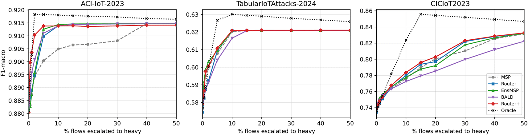
Figure 2. Routing-signal family.
F1-macro vs. % flows escalated to the heavy model (3-seed mean). Oracle (dotted) is the escalate-the-wrong upper bound. On CICIoT2023 a large oracle gap persists for all real gates.
5.3 Calibration
Figure 3 reports calibration error before and after temperature scaling, together with post-scaling reliability diagrams for all three datasets. The fitted temperatures are below one on all three datasets (
,
, and
for ACI-IoT-2023, TabularIoTAttacks-2024, and CICIoT2023), which means the tiny models are mildly underconfident and scaling sharpens their probabilities. On the two easier datasets, which are already well calibrated, scaling lowers the ECE from
to
and from
to
. On the harder CICIoT2023 the effect is inconsistent, improving two seeds but worsening one, so the mean ECE rises slightly from
to
and the reliability curve still departs from the diagonal. Calibration nonetheless matters for routing, both because the temperature-scaled confidence is among the strongest single signals in Sec. 5.2 and because comparable confidences are what let a single operating threshold behave consistently across datasets, a property we use in Sec. 5.11. On the hard task a richer scheme such as class-wise or Dirichlet calibration may behave more consistently than a single temperature, which we leave to future work.
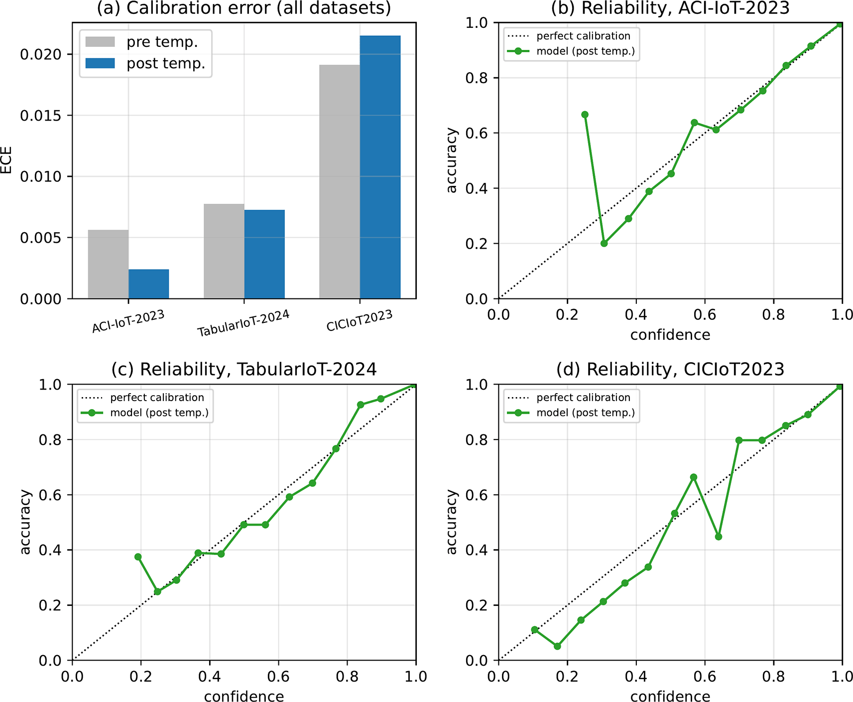
Figure 3. Calibration.
(a) Expected calibration error before and after temperature scaling for all three datasets, and (b)–(d) post-scaling reliability diagrams for ACI-IoT-2023, TabularIoTAttacks-2024, and CICIoT2023. Points on the diagonal are perfectly calibrated.
5.4 Cost-optimal, leakage-free thresholding
Table 4 reports the operating point chosen on the validation split to recover
of the heavy-tiny gap, frozen, and then evaluated on the test split. The validation-to-test selection gap is zero on all three datasets, so the validation-chosen operating point is also test-optimal. On ACI-IoT-2023 the router selects
heavy for a test F1-macro of
, matching the heavy model at a
classifier-time speedup, and TabularIoTAttacks-2024 reaches its heavy-level
at
heavy (
). CICIoT2023 instead needs
to reach
at
, short of the heavy
, which is the cost signature of its oracle gap. The zero selection gap is practically important, since it means the operating point can be fixed on validation traffic without paying a penalty on unseen traffic.
Table 4. Cost-optimal operating point chosen on validation and evaluated on test (3-seed mean).
The selection gap is the test-F1 difference between the validation-chosen budget and the best test budget. The speedup here is the classifier-only time ratio; the end-to-end speedup in
Table 10 is smaller because it also includes preprocessing.
| Dataset | %heavy | Test F1 | Heavy F1 | Speedup
|
Sel. gap |
|---|
| ACI-IoT-2023 | 8% | 0.914 | 0.915 |
| 0.000 |
| TabularIoTAttacks-2024 | 10% | 0.621 | 0.621 |
| 0.000 |
| CICIoT2023 | 33% | 0.824 | 0.834 |
| 0.000 |
Table 5. Per-comparison F1-macro difference and, in brackets, the number of seeds (of three) in which McNemar’s test is significant (
) on the shared test set.
With large test sets even a negligible F1 difference can be statistically significant, so effect size and significance should be read together.
| Comparison | ACI | TabularIoT |
CICIoT2023 |
|---|
| Dual (MSP)
tiny |
[3/3] |
[3/3] |
[3/3] |
| Router
MSP |
[1/3] |
[2/3] |
[3/3] |
| Dual (router)
heavy @10% |
[2/3] |
[2/3] |
[3/3] |
Table 6. Confidence-independent routing on CICIoT2023 (seed 42).
Test F1-macro at a matched heavy budget for MSP, two out-of-distribution latent scores (Mahalanobis, kNN), a class-reliability score, a router combining all signals, and the oracle. No practical signal approaches the oracle.
| %heavy | MSP | Maha | kNN | ClassRel | Router++ |
Oracle |
|---|
|
| 0.775 | 0.766 | 0.767 | 0.766 | 0.778 | 0.828 |
|
| 0.794 | 0.775 | 0.776 | 0.783 | 0.801 | 0.853 |
Table 7. Hardware-independent per-flow cost, as trainable parameters and forward FLOPs of the tiny path (PCA plus a
-unit MLP) and the heavy MLP.
The largest heavy
raises the ratios to
in parameters and
in FLOPs.
| Tiny path | Heavy
|
|---|
| 2–3(lr)4–5 Dataset | Params | FLOPs | Params |
FLOPs |
|---|
| ACI-IoT-2023 | 1,419 | 8.1 K | 19,723 | 39.0 K |
| TabularIoTAttacks-2024 | 1,452 | 8.2 K | 19,916 | 39.4 K |
| CICIoT2023 | 1,947 | 6.7 K | 16,027 | 31.6 K |
Table 8. Effect of heavy-model capacity (seed 42, full data,
training iterations).
For each heavy hidden size we report its parameter count, its F1-macro, the dual-path F1-macro at a
MSP budget, and the end-to-end speedup over always running heavy. As the heavy model grows, the speedup rises while the dual gate still recovers heavy-level F1.
| Dataset | Heavy size | Params | Heavy F1 | Dual F1 |
Speedup
|
|---|
| ACI-IoT-2023 |
| 20 K | 0.900 | 0.897 |
|
|
| 56 K | 0.917 | 0.913 |
|
|
| 177 K | 0.919 | 0.912 |
|
| TabularIoTAttacks-2024 |
| 20 K | 0.647 | 0.645 |
|
|
| 56 K | 0.647 | 0.646 |
|
|
| 178 K | 0.659 | 0.658 |
|
| CICIoT2023 |
| 16 K | 0.845 | 0.786 |
|
|
| 48 K | 0.856 | 0.792 |
|
|
| 162 K | 0.853 | 0.791 |
|
Table 9. Heavy backbone comparison (seed 42,
K-flow stratified subsample, multi-class).
Heavy F1-macro for an MLP
and a gradient-boosted tree (GBDT), and the dual-path F1-macro when the MSP gate escalates
of flows to the GBDT.
| Dataset | Tiny | Heavy MLP | Heavy GBDT |
Dual (GBDT, 10%) |
|---|
| ACI-IoT-2023 | 0.870 | 0.918 | 0.886 | 0.917 |
| TabularIoTAttacks-2024 | 0.573 | 0.632 | 0.662 | 0.662 |
| CICIoT2023 | 0.706 | 0.789 | 0.663 | 0.700 |
Table 10. Consolidated summary (multi-class, 3-seed mean).
Router F1/ %heavy are at the validation-chosen cost-optimal operating point; speedup is end-to-end vs. heavy; size is the heavy/tiny serialized-size ratio; ECE is post temperature scaling; the last column is dual-path F1 under coherent feature-group dropout.
| Dataset | Heavy | Tiny | Router | %heavy | Speedup
| Size ratio | ECE | dual
|
|---|
| ACI-IoT-2023 | 0.915 | 0.882 | 0.914 | 8% | 1.41
| 13
| 0.002 | 0.734 |
| TabularIoTAttacks-2024 | 0.621 | 0.574 | 0.621 | 10% | 1.37
| 12
| 0.007 | 0.520 |
| CICIoT2023 | 0.834 | 0.734 | 0.824 | 33% | 1.36
| 8
| 0.022 | 0.613 |
5.5 Statistical significance
Table 5 reports, for each comparison, the F1-macro difference and the number of seeds (of three) in which McNemar’s test finds the two classifiers significantly different on the shared test set. Dual-path gating beats the tiny model by
to
F1 in every seed of every dataset, so the core dual-path claim is unambiguous. The learned router’s edge over MSP is small in absolute terms, between
and
F1. It reaches significance on CICIoT2023 (all seeds) and, despite a negligible effect size, on TabularIoTAttacks-2024 (two seeds), whereas on ACI-IoT-2023 the larger nominal gain is not consistent across seeds. The practical message is therefore that the routing signal matters only modestly. At the
operating point the dual model is within
F1 of heavy on ACI-IoT-2023 and TabularIoTAttacks-2024 but
below it on CICIoT2023, which quantifies the oracle gap. The small differences that McNemar still flags on the two easier datasets reflect per-flow prediction changes that cancel out in macro-F1, a reminder that with large test sets significance and effect size must be read together.
5.6 The oracle gap and its mechanism
Why can confidence-based routing not reach the heavy model on CICIoT2023?
Figure 4 plots, for each class and for all three datasets, the tiny model’s confidence when wrong against its MSP-gate escalation rate. On ACI-IoT-2023 and TabularIoTAttacks-2024 almost every class is either high-accuracy or escalated when it is uncertain, so few classes sit in the dangerous bottom-right region. CICIoT2023 is different. Its high-volume denial-of-service (DoS) flood families (DoS-UDP/SYN/TCP_Flood) are wrong with high mean confidence (
to
) yet are under-escalated
(
to
, below the dataset mean), because the MSP gate reads them as confident. Confidence-based routing therefore has a structural blind spot, since it cannot catch confident errors. This is the applied, per-class manifestation in intrusion detection of a known limitation of confidence-based selective prediction,37,38 namely that a model’s own softmax cannot flag the inputs it is confidently wrong about. We observe the resulting oracle gap on the hardest of our three benchmarks; to check that it is not an artefact of the rare-class floor, we reproduce it on the merged 28-class CICIoT2023 in which no attack traffic is discarded, where the oracle still reaches an F1-macro of 0.79 at a
budget against 0.75 for MSP. The finding motivates routing on signals that are not derived from the tiny model’s own confidence, and it tempers any expectation that a better confidence gate alone can close the gap on difficult, long-tailed traffic.
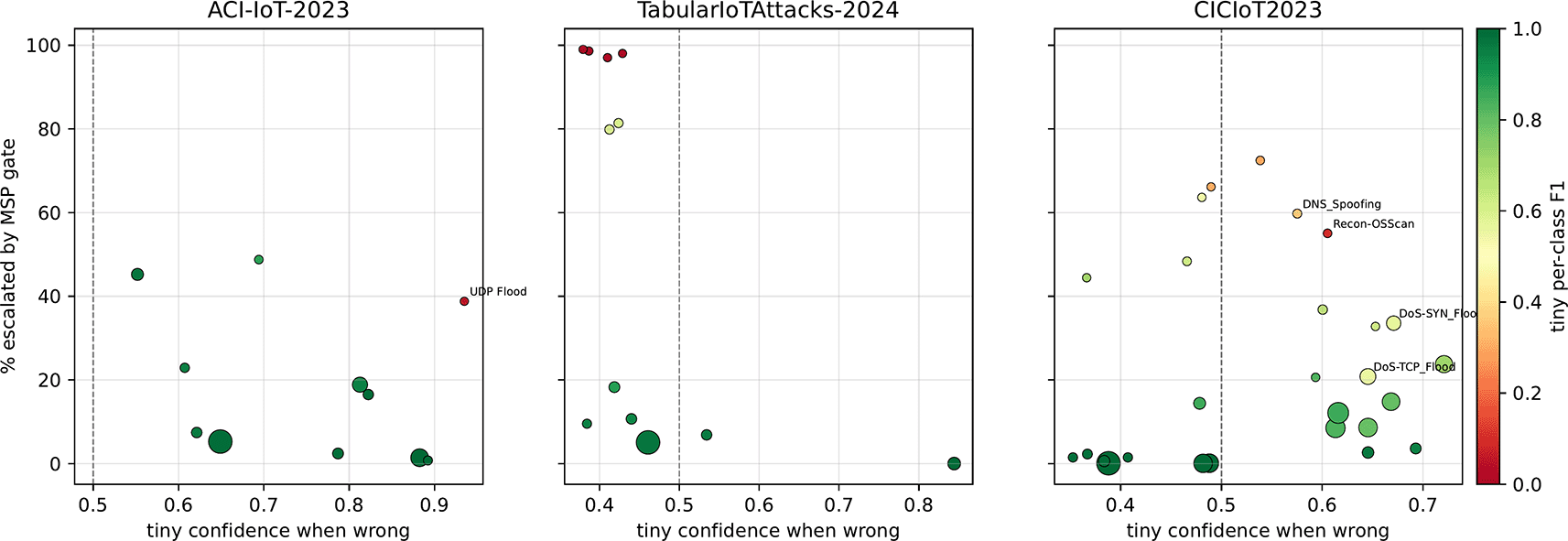
Figure 4. Oracle-gap mechanism across the three datasets.
Each point is a class, where
is the tiny model’s confidence when wrong,
is the percentage escalated by the MSP gate, marker size is class support, and color is tiny per-class F1. Only CICIoT2023 shows large, confidently-wrong classes in the bottom-right that the gate under-escalates.
Can a confidence-independent signal close the gap?
The mechanism above suggests routing on information the tiny softmax does not carry, so we test three such signals on the frozen models. Two are out-of-distribution scores in the PCA latent, a Mahalanobis distance to class-conditional Gaussians40 and the mean distance to the
nearest training latents (kNN)41; the third is a class-reliability score that escalates flows whose predicted class had low validation F1, which directly targets the failing families.
Table 6 reports CICIoT2023, and the outcome is uniformly negative. Neither out-of-distribution signal beats MSP, which shows the confident errors are in-distribution rather than outliers, and the class-reliability signal does not help either. A router that combines all signals recovers at most
F1 over MSP at large budgets, and the same pattern holds on ACI-IoT-2023 and TabularIoTAttacks-2024. Even so, the accuracy is recoverable in principle. On the very DoS-flood families that are under-escalated, the heavy model is near-perfect while the tiny model is weak, for example an F1-macro of
versus
on DoS-SYN_Flood and
versus
on DoS-UDP_Flood (this is why the oracle reaches
). The obstacle is therefore not the heavy model’s capacity but identification. The confident errors are a minority hidden inside high-volume, high-confidence classes, and no cheap signal isolates which of the many confidently-predicted flood flows are the wrong ones, whereas the oracle can because it uses the labels. The oracle gap is thus a robust identification limit of cheap per-flow routing rather than a limitation of softmax confidence alone. Closing it requires a signal that separates correct from incorrect predictions within a confidently-predicted class, which is the hard selective- prediction problem, and we leave it to future work.
5.7 Ensemble-disagreement ablation
A tiny
ensemble changes standalone F1 only marginally, from
on ACI-IoT-2023 to
on TabularIoTAttacks-2024, and its disagreement gates (EnsMSP, BALD, and Router+ in
Figure 2) beat MSP only slightly and inconsistently, and at these model sizes the ensemble’s
always-on cost approaches the heavy model’s on ACI-IoT-2023 and TabularIoTAttacks-2024 and exceeds it on CICIoT2023, with heavy-to-ensemble time ratios of
,
, and
, which removes the speedup. Epistemic disagreement does not close the oracle gap, most likely because the confident errors are agreed upon across ensemble members and so are not flagged as uncertain. We therefore retain ensembling as an ablation rather than a recommended configuration.
5.8 Robustness to feature corruption
Beyond the random per-feature dropout of the conference setting, we test coherent feature-group
“sensor outages”, where features are clustered by correlation into eight groups and whole groups are zeroed.
Figure 5 compares clean data, random
dropout, and coherent group dropout for every model and dataset, and the two corruption regimes behave differently. Under random dropout the dual model is the most robust on all three datasets, for example
on ACI-IoT-2023 against
for heavy and
for tiny, because corruption makes many flows look uncertain and the gate escalates them to the heavy path. Under coherent group outages the heavy model is instead the most robust everywhere, for example
on ACI-IoT-2023, since redundant correlated features make a whole-group loss easier to absorb than scattered noise, so heavy and tiny both degrade less than under random dropout. The dual model does not share this benefit. It stays close to the tiny model under group outages, more robust than tiny on ACI-IoT-2023 and TabularIoTAttacks-2024 but nearly tied on CICIoT2023 (
against
), and it is lower than under random dropout on the two harder datasets. This is consistent with our central finding, since a coherent outage can leave the tiny model confidently wrong, so the gate fails to escalate the affected flows.
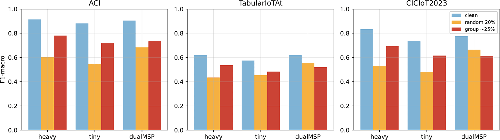
Figure 5. Robustness under clean vs. random
dropout vs. coherent group (
) dropout, per model and dataset (3-seed mean).
5.9 End-to-end latency and model size
Figure 6 reports end-to-end latency and model size. Including preprocessing (scaling + PCA), the dual-path end-to-end speedup is a modest
over heavy on all datasets, well below the classifier-only speedup, because preprocessing and the tiny forward pass are always-on. The decisive efficiency advantage is model size, where the tiny model is
smaller (
–
KB vs.
–
MB;
–
K vs.
–
K parameters). The dual system as a whole stores both models, so its footprint is dominated by the heavy model, but under offloading only the tiny model is resident on the gateway, which is where the size advantage matters most.
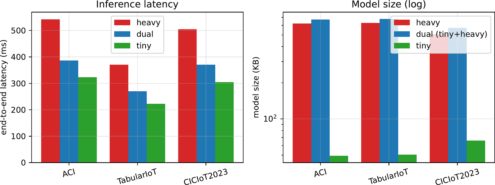
Figure 6. End-to-end inference latency (left) and serialized model size on a log scale (right), 3-seed mean.
The dual system must store both models, so its size is the sum of the tiny and heavy footprints and is dominated by the heavy model. Under offloading, only the tiny model is resident on the edge device.
Dependence on heavy-model capacity
The
end-to-end speedup above is tied to a deliberately small heavy model.
Table 8 varies the heavy hidden size from
to
and trains it for more iterations. Two effects appear. First, a larger and better-converged heavy model is more accurate, for example CICIoT2023 heavy F1-macro rises from
in the main text to
. Second, because escalation touches only
of flows, the end-to-end speedup grows with heavy capacity, reaching
to
at
on all three datasets, while the dual gate still recovers heavy-level F1. The efficiency benefit of the dual-path design therefore increases, not decreases, with a stronger heavy backbone. In hardware-independent terms (
Table 7) the tiny path uses
to
K parameters and
to
thousand floating-point operations (FLOPs) per flow, against the heavy models’
K to
K parameters and
to
thousand, a reduction of
to
in parameters and
to
in FLOPs, which bounds memory and energy on any device.
5.10 Choice of heavy backbone
On tabular data, gradient-boosted decision trees are often strong,42,43 so we also test a histogram gradient-boosting model (GBDT) as the heavy path (
Table 9). The picture is mixed. The GBDT is the strongest heavy on TabularIoTAttacks-2024 and comparable on ACI-IoT-2023, and there the dual gate recovers heavy-level accuracy at a
budget. On the hard
-class CICIoT2023, however, the GBDT underperforms even the tiny model in macro-F1, so escalating to it does not help and the MLP heavy is the better choice. Two lessons follow. First, the dual-path design and the gate operate unchanged with a non-neural heavy backbone, so the framework is not tied to neural models. Second, no single heavy family dominates across datasets, which both answers the natural GBDT baseline question and supports our use of an MLP heavy for the multi-class tasks. Because the GBDT is much slower per prediction than the tiny MLP, escalating only a small fraction keeps its use affordable where it is worthwhile.
5.11 Cross-dataset transfer of the routing policy
Can a gate tuned on one network be reused on another? Because the datasets have different feature schemas, classifiers cannot transfer, but the gate operates on dataset-agnostic confidence signals, so the question is well posed. The clearest result is a negative one. A raw MSP threshold transferred across datasets yields wildly different escalation rates, from
to
(
Figure 7), so a fixed confidence cutoff must not be reused across networks. A learned router expressed over z-scored signals does transfer, matching the in-domain router to within
F1 for every pair, but since that router is itself close to MSP (Sec. 5.2) this mainly reflects the cross-dataset comparability of calibrated confidence rather than a uniquely transferable learned policy. The practical conclusion is to set the gate by a fraction or budget target, which is portable, rather than a raw threshold, which is not.
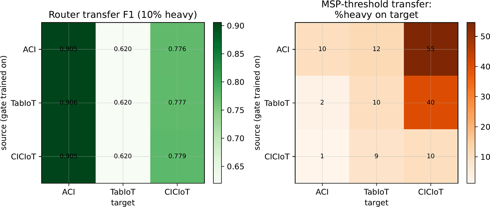
Figure 7. Cross-dataset transfer.
On the left, router-transfer F1 (uniform columns indicate source-independence). On the right, the heavy fraction induced on the target by a source-chosen MSP threshold (large off-diagonal values indicate no transfer).
6 Discussion
Table 10 collects the main numbers, and one result stands out. Routing a small fraction of flows to a heavy model recovers most of its accuracy, and this is the one large and statistically significant win. The choice of signal, by contrast, matters little. A learned router is the best practical gate, but its edge over MSP is small, and ensemble-averaged confidence is a simple alternative that never does worse. Confidence-based routing also has a hard ceiling. On long-tailed multi-class traffic the confident errors on a few attack families stay invisible to confidence, disagreement, out-of-distribution, and class-reliability signals alike, so accuracy is capped below the heavy model whatever the budget. The efficiency story is more about size than speed, since the tiny path is roughly ten times smaller but only about
faster end to end. And a fixed confidence threshold does not carry across networks, though a fraction or budget target does, so the gate policy itself stays portable. We tested routing signals independent of the tiny model’s confidence, namely latent-space out-of-distribution scores and class-aware escalation (Sec. 5.6), and found that they do not close the oracle gap either. Because the heavy model is already near-perfect on the failing families, the obstacle is identification rather than capacity. Closing the gap requires a signal that separates the minority of confident errors from the majority of correct predictions within a high-confidence class, which is the hard selective-prediction problem, and we leave it to future work.
Deployment recipe
For a practitioner the results reduce to a short recipe. Run a tiny PCA-latent model on the edge gateway and expose a stronger model, either a larger MLP or a gradient-boosted tree whichever is stronger on the target traffic (Sec. 5.10), as the escalation target on a more capable node. Calibrate the tiny model and route by a fixed escalation budget, chosen on validation to match the available heavy-compute headroom, rather than by a fixed confidence threshold, since thresholds do not transfer across networks. Plain MSP is an adequate routing signal, so a learned router is optional and worth at most a fraction of a point. Expect near-heavy accuracy at a small budget on easy traffic, and plan for a larger escalation fraction, or accept a residual gap, on hard long-tailed traffic where confident errors evade the gate.
7 Limitations and threats to validity
All timing is on a workstation CPU and is implementation-dependent, so we report relative comparisons and serialized sizes; on-device latency and energy on representative edge hardware, for example a Raspberry-Pi-class gateway, are future work, although the parameter and FLOP reductions in Sec. 5.9 bound the achievable gain on any device. The rare-class floor on CICIoT2023 drops 7 of 34 classes for the main results; to confirm this does not change our conclusions, we also ran a variant that merges those classes into a single Other_Attack class so that no attack traffic is discarded, and the ordering is preserved (heavy, tiny, and dual F1-macro of
,
, and
over 28 classes, against
,
, and
when dropped, 3-seed means). The main-text heavy model is a moderate MLP
trained for few iterations;
Table 8 shows that a larger and better-converged heavy model is both more accurate and yields a larger end-to-end speedup, so our headline
is a conservative lower bound rather than a ceiling. Cross-dataset transfer is evaluated over bounded confidence signals on which the learned router is close to MSP, so the positive transfer partly reflects MSP’s universality. Feature-group “outages” are approximated by correlation clustering rather than ground-truth sensor metadata. Finally, the multi-seed statistics use three seeds, and McNemar significance on large test sets should be read together with effect size, as discussed in Sec. 5.5.
8 Conclusion
We presented a systematic study of the escalation gate in dual-path lightweight IoT intrusion detection across three benchmarks. Confidence-gated conditional computation delivers large, significant accuracy recovery at low cost. In practice a simple budget-controlled MSP gate is sufficient, and a learned, calibration-aware router adds only small gains over it while providing a leakage-free operating point; the routing policy, expressed over normalized signals, transfers across networks. Our central, honestly-reported finding is an oracle gap on hard multi-class IoT traffic, mechanistically explained by confident errors on high-volume attack families that no cheap routing signal we test catches, whether confidence-based, ensemble-disagreement, out-of-distribution, or class-reliability. Because the heavy model is already near-perfect on the failing families, this gap is an identification problem rather than a capacity one. These results give practitioners concrete guidance and single out the identification of confident errors within high-confidence classes, a selective-prediction problem, as the key open problem for adaptive IoT IDS.







