Introduction
Researchers often seek to clarify relationships between two categorical variables. For example, statistical tests are commonly used to assess whether two proportions differ across two sampled populations. In public health and the social sciences, such comparisons frequently concern sex, gender, ethnic group, socioeconomic status, or behavioural categories.1–4 The conventional approach is the frequentist framework. In practice, this involves setting a Type I error threshold, usually at 5%, selecting an appropriate test, and comparing the resulting p-value with that pre-specified threshold.5 Additional indicators, such as effect size and statistical power, are sometimes reported as well.6,7 By design, frequentist tests focus on a test statistic whose distribution is known under the null hypothesis of no effect. The p-value therefore corresponds to the probability of observing data at least as extreme as those obtained, assuming that the null hypothesis is true.8
However, as highlighted by Dablander et al. (2022) and Keysers et al. (2020), frequentist hypothesis tests can provide evidence for an association when the null hypothesis is rejected, but when it is not rejected, they indicate only an absence of evidence.8,9 As discussed by Altman and Bland (1995), failure to reject the null hypothesis should therefore not be interpreted as confirmation that no association exists.10 This situation is particularly common in studies based on small sample sizes, where limited statistical power reduces the ability to detect true effects.8
Although minimum sample sizes can be estimated from assumptions about power and effect size,6,11 logistical or resource constraints may prevent researchers from reaching the recommended sample size.12 Geographic remoteness, scarcity, and population dispersion make some populations particularly difficult to study. Research conducted in Pacific Island Countries and Territories (PICTs) exemplifies many of the structural constraints associated with small-sample research. Geographic isolation, population dispersion across multiple islands, and limited local research infrastructure often restrict achievable sample sizes.13 In addition, individual islands may have only a few thousand inhabitants.14,15 In this contexts, conventional hypothesis testing frequently produces non-significant results, not necessarily because associations are absent, but because the available data do not contain enough information to meet conventional decision thresholds.
This situation is especially problematic in public health research, where small populations are often those experiencing a disproportionate burden of disease and where evidence is most urgently needed to inform policy and intervention. Indeed, PICTs face a rapidly increasing burden of non-communicable diseases, including overweight and obesity in both adults and children.16,17 The combination of high public health relevance and limited statistical power underscores the need for analytical frameworks that can extract meaningful information from small datasets.
As an example, Bertrand-Protat et al. (2024) presented data on an understudied child population in Wallis following a school-based physical activity promotion programme.18 Of the 52 pupils who consented to participate, only 32 participants with complete data were included in the reported analyses. Although the authors conducted frequentist tests, they were able to report only descriptive results without statistical significance.18 Those results nevertheless did not justify concluding that the data supported the null hypothesis, especially given the particularly small sample size.8,10 This example illustrates the critical need to reconsider how evidence from small-sample studies is analysed and interpreted in Pacific research, and more broadly in social sciences.19 Methodological approaches that allow a more nuanced interpretation of results obtained from small samples are therefore essential to ensure that research conducted in such settings is not systematically undervalued.
For its part, the Bayesian testing framework offers additional indicators, such as weighted evidence for or against the hypotheses under consideration, derived from Bayes factors.8,20–22 Examination of posterior densities and the credible intervals (CI) for the relevant parameters also provides valuable information. Unlike the frequentist framework, which relies solely on assumptions related to the null hypothesis, the Bayesian approach also requires an explicit formulation of the alternative hypothesis and an updating step based on that formulation and the observed data.8 In small-sample contexts, this distinction is particularly important because non-significant p-values are common and are often misinterpreted. Furthermore, Bayesian methods make it possible to distinguish between absence of evidence and evidence of absence.10 By presenting both frequentist and Bayesian results side by side, this study illustrates how the two frameworks can jointly support a more informative and transparent interpretation of empirical findings.
This study provides an overview of Bayesian A/B testing, with a particular emphasis on the interpretation of its outputs, thereby demonstrating its usefulness for researchers comparing two proportions in small-sample settings. We implement both the Independent Beta Estimation (IBE) and the Logit Transformation Testing (LTT) approaches using several R-based implementations or computational strategies (IBE: 3; LTT: 2). These approaches will be applied to data from an empirical study conducted in a PICT in order to examine the association between parental weight status and child weight status. Because small samples can be highly sensitive to minor changes in the data, we also investigate the effect of slight data alterations on the results.
The Materials and methods section first describes the case study context. It then briefly reviews the frequentist framework - specifically the Fisher’s exact test, which is commonly used in such situations - and the Bayesian framework, focusing on the IBE and LTT approaches. The priors selected for the Bayesian analyses are then detailed, and the section concludes with a description of the Bayes factor calculations. The results are subsequently presented and finally discussed.
Material and methods
Move Ô study: context and dataset
The Move Ô protocol was developed to generate actionable evidence for policymakers addressing childhood obesity in Pacific Island contexts. Its primary objective was to examine a broad range of determinants of childhood overweight and obesity, including factors that are well established internationally - such as unhealthy dietary patterns, physical inactivity and sedentary behaviour, insufficient sleep, parental body weight, and socioeconomic conditions - but that have so far been insufficiently studied in the Pacific region.18 The study was conducted among all Grade 5 students (CM2 in French school system) from four schools on Wallis Island. A total of 52 children aged 9 to 11 years participated in the study in March 2024. Data were collected using multiple complementary methods, including questionnaires, wrist-worn accelerometers, interviews, and direct observations. The study received approval from the New Caledonia Ethics Advisory Committee and complied with the Declaration of Helsinki.
Children’s weight was measured using a SECA 813 scale, and their height was measured with a SECA 213 stadiometer. Parental height and weight were collected by questionnaire, which asked: “Please provide the following information about the child’s father (respectively, the child’s mother): height: … ; weight: …”. Only participants with complete height and weight data for both the child and the parents were included in the present analysis, yielding a final sample of 27 participants.
Weight status categorisation
Body mass index (BMI) for both children and adults was calculated from weight in kilograms and height in metres as follows:
(1)
Adults were classified as either “Underweight or Normal range” or “Overweight or Obese” in accordance with World Health Organization guidelines23: “Underweight or Normal range” if
, and “Overweight or Obese” if
. Children were classified using the International Obesity Task Force reference.24 As for adults, the children were grouped into two categories: “Underweight or Normal range” and “Overweight or Obese”.
Definitions and notations
Group 1 comprised children with at least one parent in the “Underweight or Normal range” category, whereas Group 2 comprised children whose parents were both “Overweight or Obese”.
We denote:
•
the total number of observations and
the number of successes (i.e. the number of overweight or obese children) in Group 1;
•
the total number of observations and
the number of successes (i.e. the number of overweight or obese children) in Group 2;
•
the true proportion of successes among children in the population whose parents are not both overweight or obese (i.e. the population with characteristics similar to Group 1);
•
the true proportion of successes among children in the population whose parents are both overweight or obese (i.e. the population with characteristics similar to Group 2);
•
,
, the sample estimates of the true success proportion
.
In hypothesis testing, the plausibility of two competing propositions is compared. The null hypothesis assumes equal proportions. The four alternative hypotheses considered are as follows:
•
•
•
•
When comparing two proportions, it is also common to report an effect size,6 denoted
, defined as follows:
(2)
Reminder about the frequentist methods and the Fisher’s exact test
Frequentist hypothesis testing assesses whether the observed data is statistically compatible with the null hypothesis of “no effect”.5 When comparing two proportions, this approach typically involves testing the null hypothesis of equality between groups against an alternative hypothesis specifying a difference. Researchers are primarily interested in the p-value, i.e. the probability of observing data as extreme as, or more extreme than, those observed, assuming that the null hypothesis is true. This p-value is then compared with a pre-specified significance threshold, which is most commonly set at 0.05. Although widely used, this framework does not provide a direct measure of evidence in favour of the null hypothesis and can be difficult to interpret in small-sample situations.
Fisher’s exact test is a non-parametric statistical test commonly used to assess the association between two categorical variables in contingency tables, particularly when small sample sizes make the standard
large-sample test unreliable. Based on the hypergeometric distribution, this test computes the exact probability of observing a difference at least as extreme as the one obtained under the null hypothesis, i.e. a difference that can be explained by chance.25 In the present study, Fisher’s exact test is applied in both two-sided and one-sided forms to compare the proportions of overweight or obese children between the two parental weight-status groups. As with other frequentist tests, failure to reject the null hypothesis should be interpreted as an absence of evidence rather than evidence of no association.
Principles of the Bayesian A/B testing models
A binomial model is used to describe the number of overweight or obese children in each group, i.e.
in Group 1 and
in Group 2:
(3)
Where
denotes the binomial distribution and
,
, represents the underlying probability of success in group
. The aim is to infer plausible values for
,
and to quantify the evidence supporting competing hypotheses about their relationship.
In the Bayesian approach, the analysis begins with prior distributions, which reflect the experimenter’s beliefs or knowledge about the parameters of interest (i.e.
) before data collection.19,26 Priors may be non-informative, reflecting limited prior knowledge, or informative, reflecting external evidence or strong expectations about the parameters.3 Once the data have been collected, each prior is updated to a posterior distribution (
Figure 1), which then helps determine which hypothesis is better supported.
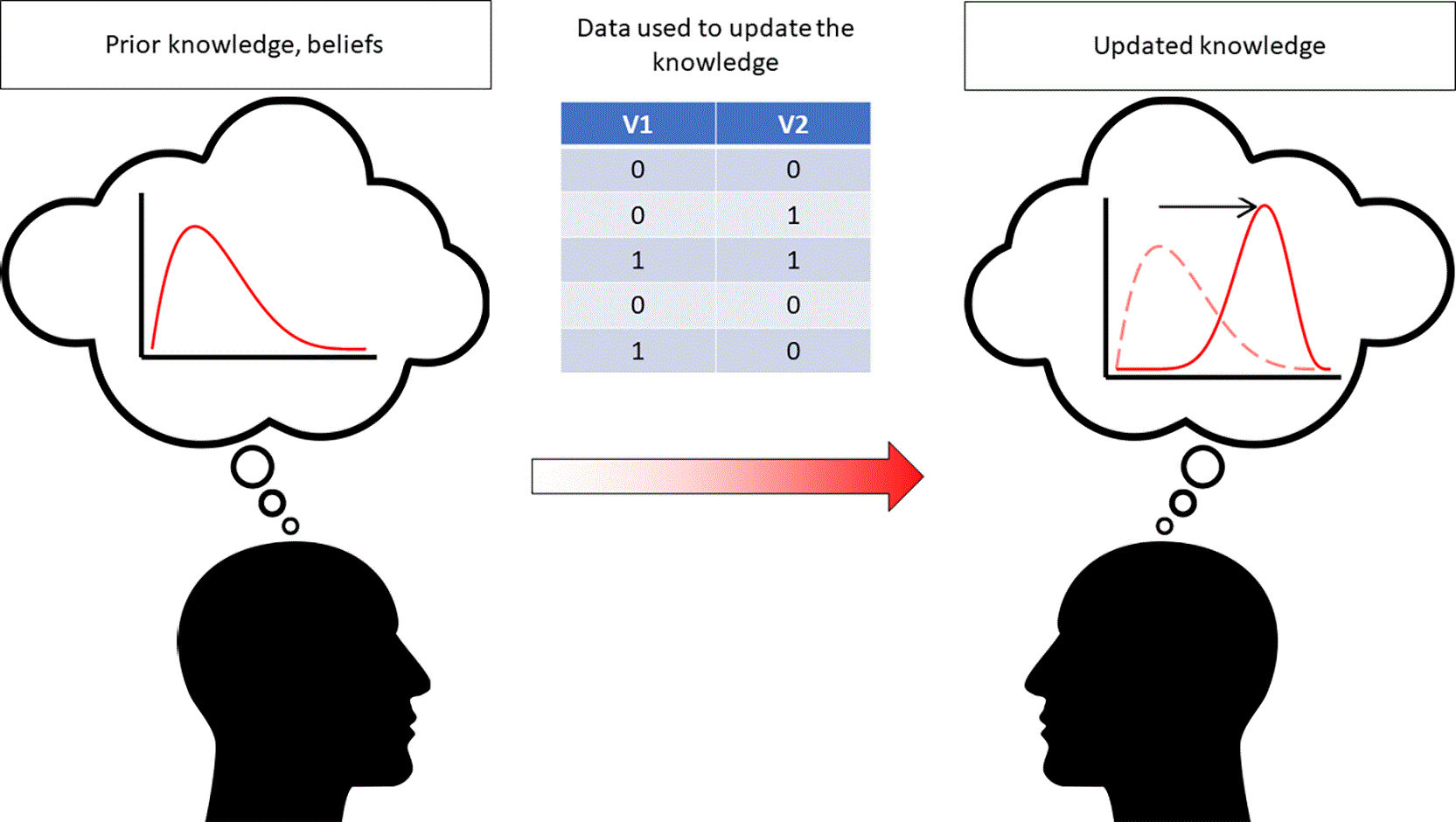
Figure 1. Diagram illustrating the principles underlying the Bayesian tests.
Within the Bayesian framework, the strength of evidence favouring one hypothesis over another is quantified by the posterior odds. This quantity is related to the Bayes factor, as shown in the following equation used to compare
and
21,27
(4)
In this equation,
and
are the posterior probabilities of
and
, respectively, whereas
and
denote the prior probabilities, based on beliefs and knowledge, of
and
, respectively. The Bayes factor is denoted as
.
The two approaches considered in this paper, namely IBE and LTT, are based on distinct models and therefore on different families of prior distributions, which in turn lead to different posterior distributions.
Independent Beta Estimation (IBE) approach
Although readers can find a detailed description of the IBE approach in Hoffmann et al. (2022),3 we reiterate the main points here.
In the IBE approach, the distributions of
and
are assumed to be independent, just as the success probabilities are assigned independent
distributions:
,
. These distributions model the relative plausibility for
,
, with the
and
parameters interpreted as counts of hypothetical successes and failures, respectively.
At the outset, prior distributions, denoted as
, are selected on the basis of the experimenter’s knowledge, or lack thereof, and therefore be informative or non-informative. The data collected during the experiment are then used to update the prior distributions into posterior distributions, according to Bayes’ rule for
:
(5)
where
represents knowledge of the number of observations (i.e.
) and the number of successes (i.e.
) derived from the observed data;
is the probability deduced from
;
arises from the binomial distribution of the data; and
is the likelihood of the data given the parameter
.
In this approach, since the prior distributions are
distributions with parameters
, the posterior distributions become
distributions with parameters
, where
is the number of observed successes and
the number of observed failures.28 However, as pointed by Gronau et al. (2021) and Dablander et al. (2022), this test does not allow the experimenter to assess exact equality of the proportions.9,29 In practice, it therefore amounts to comparing
and
.
To characterise prior and posterior uncertainty, we rely on simulation from
distributions using standard R functions,30,31 together with results obtained from the bayesAB package and from Markov chain Monte-Carlo (MCMC) estimation via the R2jags package in order to verify consistency across computational strategies.19,30,32–36 R version 4.4.2 was used in the present study.
In the results, we consider the computed and simulated distributions of the parameters of interest, i.e.
and
. Given its great interest, we also examine the assessment of the difference between the proportions, denoted
, and estimate the 90% highest density interval (HDI) and equal-tailed interval (ETI) for the credible interval (CI),37 the posterior probability
, and the Bayes factors
.
Logit Transformation Testing (LTT) approach
As in the previous subsection, readers can refer to Hoffmann et al. (2022) for a comprehensive description of the LTT approach.3 However, we summarise the main elements hereafter.
The LTT approach is based on a model described by Kass and Vaidyanathan (1992),38 who proposed a test applied to the log-odds transformation of the parameters of interest, namely
and
. The model is thus expressed as follows:
(6)
where
denotes the grand mean of the odds ratio and
represents the distance between the two conditions.
39 By default, both parameters are assumed to follow Gaussian distributions:
and
. Within this framework, the hypotheses to be tested can be written as follows:
•
•
•
•
Updating the
parameters then yields posterior distributions, modal estimates for the parameters of interest
, and Bayes factors for hypothesis comparison.
Results from the implementation included in the abtest R package are presented in this paper.29 In addition, we incorporate information from the R2jags outputs used in the LTT approach.33 In that implementation, however, we chose to not use truncated distributions, unlike the abtest R package. In the results, we consider the outputs from abtest, which provide information on Bayes factors (
and
), posterior probabilities (
versus
or
), 90% CI, and robustness analysis.29 We also examine the distributions of the parameters of interests and the difference
.
Choices of prior distributions
To reflect realistic analytical practice and recommendations in the methodological literature, we examine multiple prior scenarios rather than relying on a single prior specification.3,19,31 This is particularly important in our small-sample settings, where inferential summaries - especially Bayes factors - can be sensitive to prior choices.8 Accordingly, we investigate three scenarios: non-informative, informative, and optimistic. These scenarios are intended to span a reasonable range of prior knowledge and expectations relevant to childhood overweight and obesity in Pacific settings.
Before describing the priors used in the three scenarios (non-informative, informative, and optimistic), it is worth noting that, in the LTT approach, the central values of both
and
can be derived from the beliefs and knowledge available - or unavailable - about the primary parameters (i.e.
and
), according to the following relationships.
(7)
For the non-informative scenario in the IBE approach, every value between 0 and 1 is, a priori, equally possible for the success proportion (i.e. overweight or obese) in each of the two groups under study. Two
distributions therefore provide an appropriate prior specification, which is equivalent to using two uniform distributions defined on
(
Figure 2). In the LTT approach, the absence of prior knowledge can be modelled by values of
and
distributed around 0.5. Consequently, choosing two
distributions for both
and
is appropriate for this prior (
Figure 2).
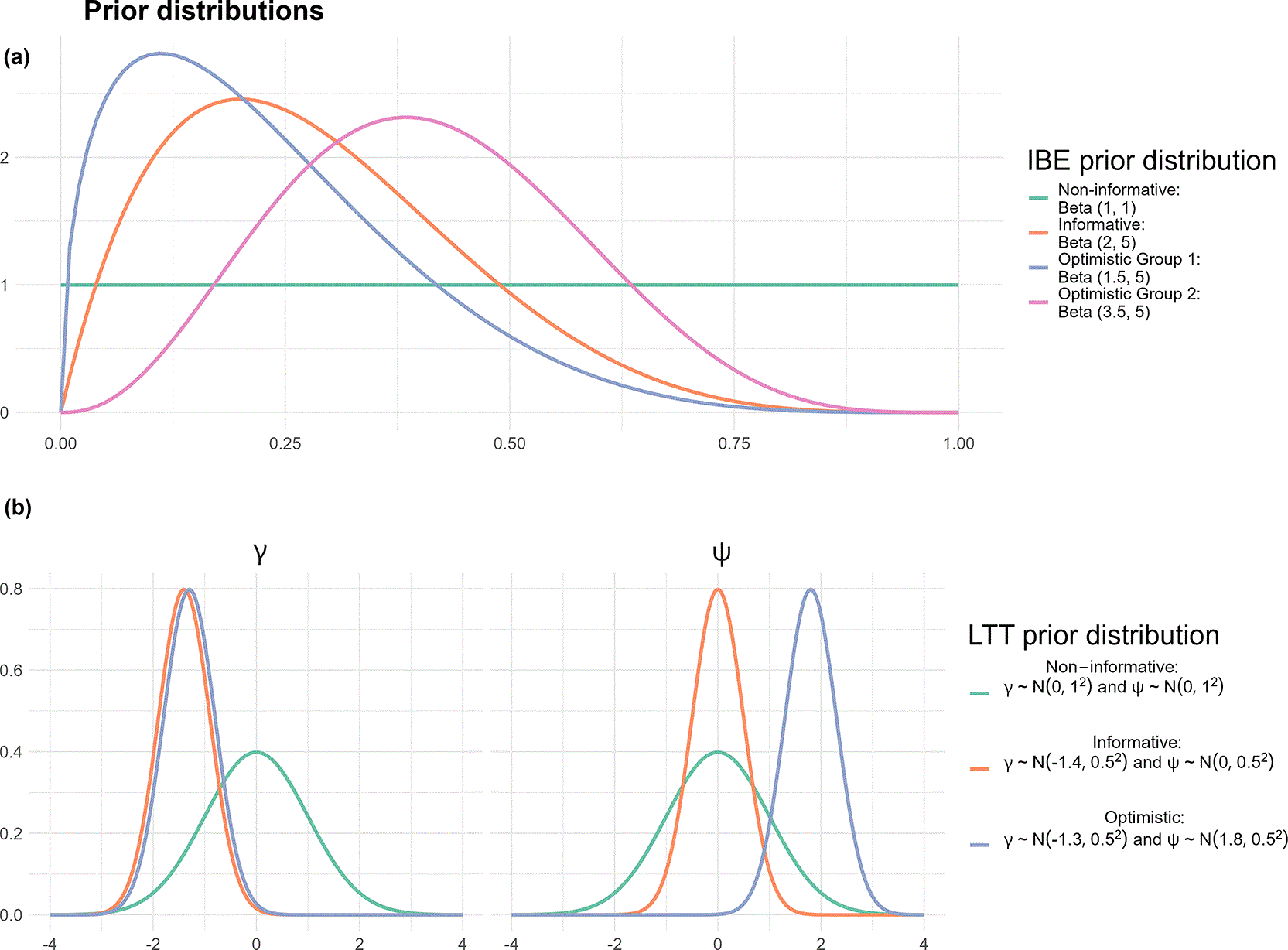
Figure 2. Prior distributions used in the present study for each scenario investigated (1. Non-informative, 2. Informative, 3. Optimistic): (a)
distributions used to estimate the
and
parameters in the IBE approach, (b) Normal distributions used to estimate the
and
parameters in the LTT approach.
When selecting an informative prior distribution, the experimenter must draw on prior beliefs and knowledge.26,40 Recent studies suggest that approximately 20% to 30% of young people in the considered populations are affected by this health issue.17,41 This information guides the choice of the parameters of the
distribution so that the density peaks around these values. For example, using two
distributions in the IBE approach, with substantial mass around 0.2, is consistent with previous observations (
Figure 2). In the LTT approach, if the researcher does not distinguish Groups 1 and 2, the underlying belief is that
. From
Equation 7, we deduce:
(8)
This is why using a Gaussian distribution centred at −1.4 for
and another centred at 0 for
appears reasonable. The standard deviation can be set to 0.5 in order to limit dispersion, yielding the following prior distributions (
Figure 2).
(9)
For the optimistic scenario, the experimenter again relies on prior beliefs and knowledge.26,40 For genetic or environmental reasons, it is reasonable to expect that a child in Group 2 (whose parents are both overweight or obese) is much more likely to be overweight than a child in Group 1 (with at most one parent who is overweight or obese).42–44 In the IBE approach, this scenario is modelled by two priors depending on the group. The experimenter could therefore select a
distribution, with substantial mass around 0.1, for Group 1, and a
distribution, with substantial mass around 0.4, for Group 2 (
Figure 2).
From
Equation 7, with
and
, we obtain in the LTT approach:
(10)
Consequently, using a Gaussian distribution centred at −1.3 for
and another centred at 1.8 for
appears reasonable. As in the informative scenario, the standard deviation can be set to 0.5 in order to limit dispersion, yielding the following prior distributions (
Figure 2).
(11)
Calculation of Bayes factors
In the IBE approach, it is possible to compare the evidence supporting either
or
9 The resulting Bayes factor,
, was computed as follows:
(12)
where
and
are the posterior probabilities respectively for
and
respectively, and
and
are the prior probabilities, estimated from the number of simulated values supporting
and
, respectively, under the prior
distributions. Similarly, the posterior probabilities were estimated by the number of simulated values supporting
or
under the posterior
distributions.
In the LTT approach, the ab_test function from abtest R package provides estimates of Bayes factors in favour of
over
,
over
and
over
29 When using the MCMC simulations generated with the R2jags package, the Savage-Dickey method was used to estimate
, from which
was then derived.31,45 The remaining Bayes factors, i.e.
and
, were subsequently calculated from the estimates of
and from the prior and posterior probabilities46:
and
.
When comparing
and
, the Bayes factor was estimated as
, and the posterior probability was estimated as
.
Application results
Results of the Fisher’s exact test for the Move Ô case study
Table 1 presents the contingency table summarising the distribution of the successes across the two groups. From this table, the estimates of
and
are
and
, respectively. Likewise the estimates of
and
are
and
, respectively, yielding
, which corresponds to a large effect size.6
Table 1. Distribution of successes (overweight or obese) and failures (underweight or normal) for each Group (1: parents are not overweight or obese together; 2: both parents are overweight or obese) for the Move Ô case study.
| Group 1 [n (%)] |
Group 2 [n (%)] |
|---|
| Underweight or normal | 5 (83) | 10 (48) |
| Overweight or obese | 1 (17) | 11 (52) |
Applying the two-sided Fisher’s exact test, i.e. testing
against
, yielded
; therefore
was not rejected. Under the frequentist framework, the data therefore provide no evidence of a significant difference between the two groups. Applying the one-sided Fisher’s exact test, i.e. testing
against
, yielded
; again
was not rejected. As in the two-sided analysis, the data therefore provide no evidence of a significant difference between the two groups.
Results of the IBE approach for the Move Ô case study
We now turn to the IBE and LTT approaches. Under the IBE approach, the posterior distributions can be derived directly from the prior specification and the observed data.
Table 2 summarises the prior and posterior distributions for Groups 1 and 2 under the three scenarios investigated, namely the non-informative, informative, and optimistic scenarios.
Figure 3 shows the shape of each distribution, and
Figure 4 presents the distributions of the difference
simulated under both the prior and posterior settings.
Table 2. Prior and posterior distributions according to the investigated scenario (1. Non-informative, 2. Informative, 3. Optimistic) and the Group in the IBE approach applied on the Move Ô case study.
| Prior distribution | Posterior distribution |
|---|
| Group 1 | Group 2 | Group 1 | Group 2 |
|---|
| Non-informative
|
|
|
|
|
| Informative |
|
|
|
|
| Optimistic |
|
|
|
|
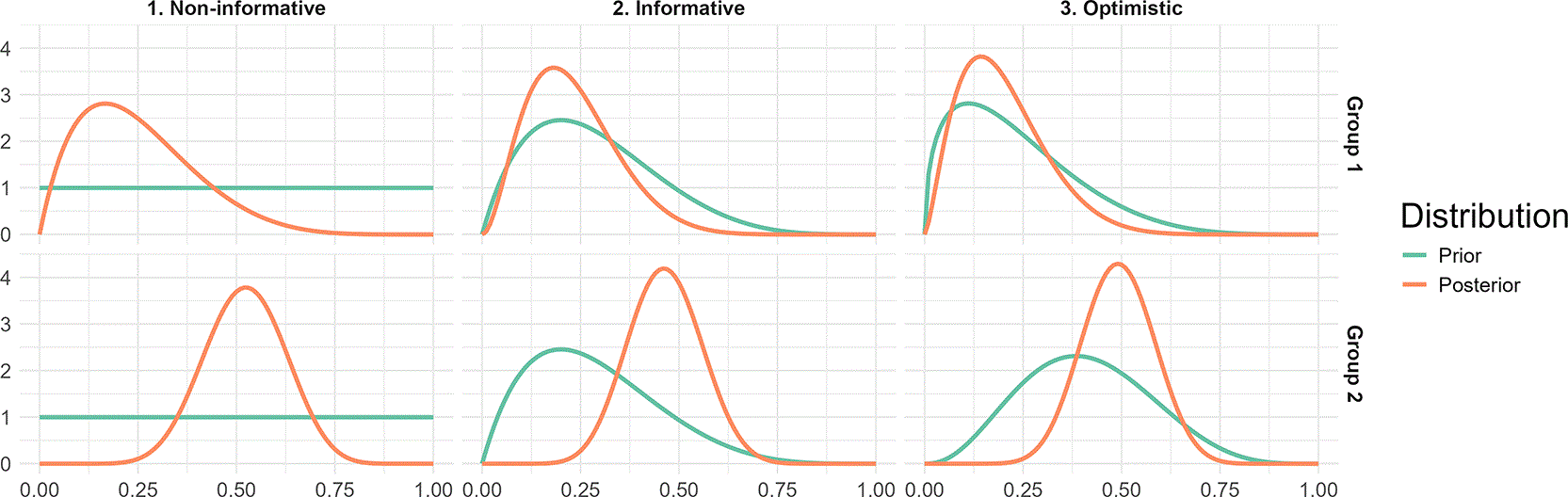
Figure 3. Prior and posterior
distributions of the IBE approach applied on Groups 1 (upper row) and 2 (lower row) for the Move Ô case study for each scenario investigated: 1. Non-informative, 2. Informative, 3. Optimistic.
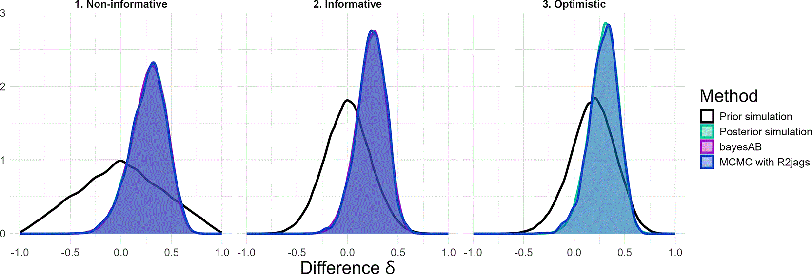
Figure 4. Distributions of the difference (
) simulated in the prior and posterior settings for the Move Ô case study by the three implementations (our own simulation coding, bayesAB package, and MCMC with R2jags) of the IBE approach for each scenario investigated: 1. Non-informative, 2. Informative, 3. Optimistic.
Figure 3 clearly shows how the density curves change once the sample information is incorporated. In the non-informative scenario, the flat prior distributions become posterior distributions with pronounced peaks. Overall, the choice of scenario (non-informative, informative, and optimistic) did not substantially alter the general shape of the posterior distributions or their main indicators. In the non-informative scenario, the posterior density peaked at approximately 0.18 in Group 1 and 0.52 in Group 2. In the informative scenario, the corresponding modes were approximately 0.19 and 0.46. In the optimistic scenario, they were approximately 0.15 for Group 1 and 0.49 for Group 2. In all scenarios, the support of the density was wider for Group 1 than for Group 2 because the sample size was smaller in Group 1.
Figure 4 shows that, regardless of the method or the package used, the posterior distributions of
were broadly similar, although the posterior distribution was more diffuse in the non-informative scenario. In the non-informative scenario, the prior distribution peaked around 0 and the posterior distribution around 0.32. In the informative scenario, the prior again peaked around 0, whereas the posterior peaked around 0.28. In the optimistic scenario, the prior peaked around 0.21 and the posterior around 0.31.
Table 3 reports the posterior probabilities
and the Bayes factors
, allowing the comparison of the three implementations of the IBE approach across the non-informative, informative, and optimistic scenarios. Table S1 complements these results by reporting the quantiles and the 90% CI of the parameter distributions (
,
, and
). Across all scenarios, the three methods yielded equivalent highly similar results. For example, the only posterior quantiles that differed at the second decimal place were approximately the 0% and 100% quantiles (Table S1). The posterior probabilities
showed only minor variations for the MCMC implementation with R2jags, at the second decimal place in the optimistic scenario. Indeed, they ranged from 0.925 to 0.926 in the non-informative scenario, from 0.937 to 0.938 in the informative scenario, and from 0.971 to 0.972 in the optimistic scenario. The Bayes factors
, rounded to the nearest whole number, were consistent across methods and indicated moderate to strong evidence for
over
: from 12.360 to 12.585 in the non-informative scenario, from 14.814 to 14.898 in the informative scenario, and from 8.501 to 8.616 in the optimistic scenario.21 However, as noted by Dablander et al. (2022),9 Bayes factors computed under the IBE approach are often optimistic.
Table 3. Prior probabilities
, posterior probabilities
and Bayes factors
estimated by the three implementations (i.e., our own simulation, bayesAB package, and MCMC with R2jags) of the IBE approach for the Move Ô case study in the three scenarios investigated: 1. Non-informative, 2. Informative, 3. Optimistic.
| | Non-informative
| Informative | Optimistic |
|---|
| Theoretical prior probability
| 0.500 | 0.500 | |
| Analytic posterior probability
| 0.926 | 0.937 | 0.972 |
| Simulation | Prior probability
| 0.500 | 0.503 | 0.800 |
| Posterior probability
| 0.925 | 0.938 | 0.972 |
| Bayes factor
| 12.360 | 14.859 | 8.616 |
| bayesAB package | Posterior probability
| 0.926 | 0.937 | |
| Bayes factor
| 12.585 | 14.898 | |
| MCMC with R2jags | Posterior probability
| 0.926 | 0.937 | 0.971 |
| Bayes factor
| 12.490 | 14.814 | 8.501 |
Results of the LTT approach for the Move Ô case study
Figure 5 displays the simulated distributions of the parameters of interest, i.e.
,
,
and
, as well as the simulated distributions of the difference
.
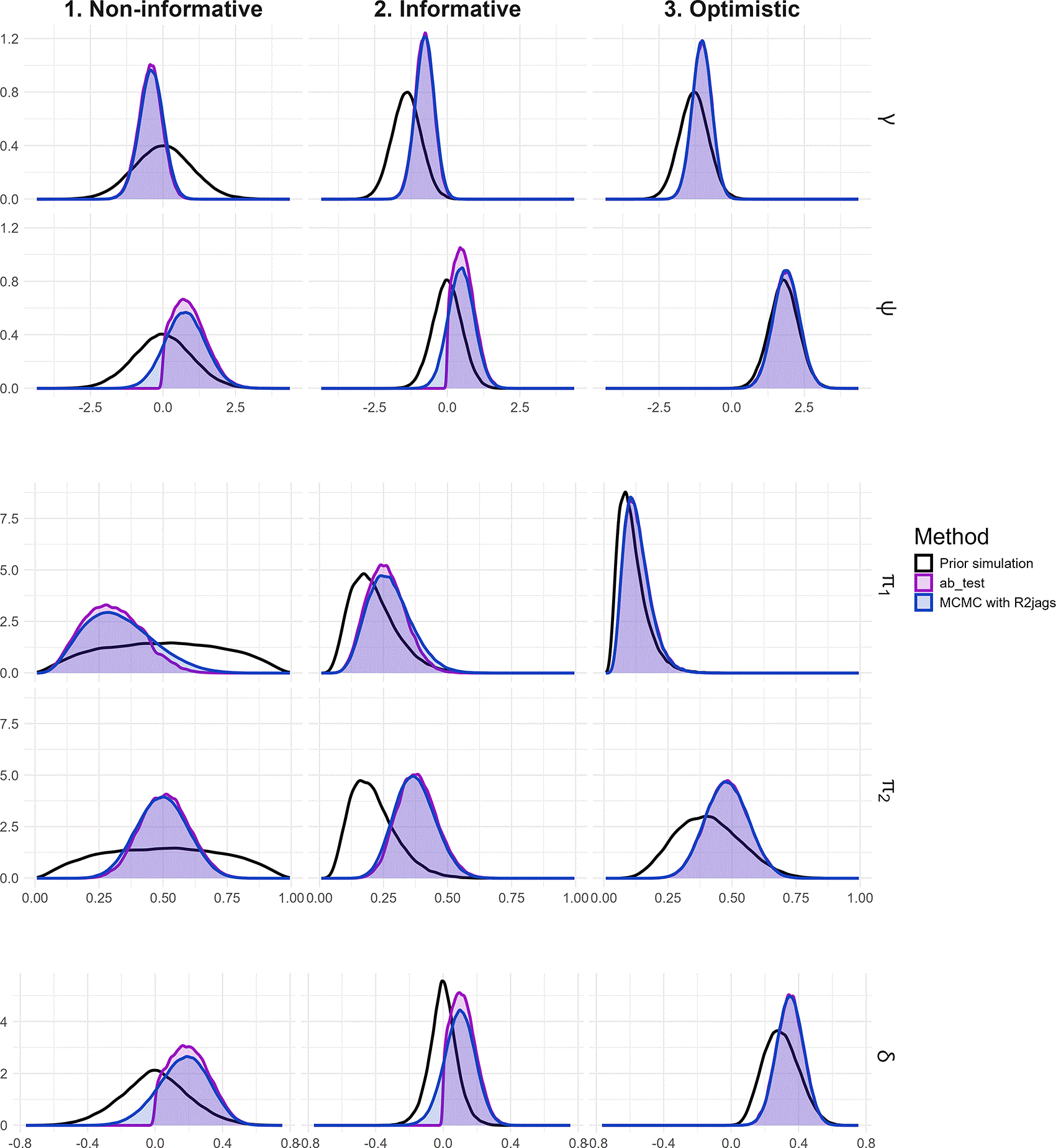
Figure 5. Distributions of the
,
,
and
parameters and the difference
simulated under the prior and posterior settings for the Move Ô case study by the two implementations (ab_test from abtest package, and MCMC with R2jags) of the LTT approach for each scenario investigated: 1. Non-informative, 2. Informative, 3. Optimistic.
The
distributions depicted in
Figure 5 shift towards negative values, with modes around −0.43 in the non-informative scenario, −0.77 in the informative scenario, and − 1.00 in the optimistic scenario. This shift reflects an overall probability of success (i.e. the proportion of participants who were overweight or obese) ranging between 0.27 and 0.39, which was also a central value between
and
. The main focus, however, is the
distributions, because they represent the magnitude of difference between
and
. Their mode is positive in all scenarios, at approximately 0.75 in the non-informative scenario, 0.50 in the informative scenario, and 1.90 in the optimistic scenario. These values were the maximum likelihood for the logit difference according to the respective scenario.
The
distributions show different modal values across the scenarios investigated: 0.28 in the non-informative scenario, 0.24 in the informative scenario, and 0.10 in the optimistic scenario. The greatest variability was observed in the non-informative scenario, while the smallest variability was observed in the optimistic scenario. The modal values of
were 0.50 in the non-informative scenario, 0.37 in the informative scenario, and 0.48 in the optimistic scenario. In every scenario, the posterior distributions were more peaked than the corresponding prior distributions.
The modal values of
shown in
Figure 5 were 0.17 in the non-informative scenario, 0.10 in the informative scenario, and 0.34 in the optimistic scenario, thereby characterising the difference between
and
. The highest distribution peak was observed in the informative scenario, whereas the lowest occurred in the non-informative scenario.
No major differences were observed between the two methods (i.e. abtest and MCMC with R2jags) except for the
and
distributions in the non-informative and informative scenarios. These discrepancies arose because abtest uses a truncated distribution, whereas our MCMC implementation imposed no such constraint.
Table 4 reports the posterior probabilities and Bayes factors obtained from the two implementations of the LTT approach across the scenarios investigated. The hypothesis
was compared first with
and then with
. Table S2 complements these results by reporting the quantiles and 90% CI of the parameter distributions considered (
,
,
,
, and
).
Table 4. Prior probabilities, posterior probabilities and Bayes factors estimated by the two implementations (abtest package, and MCMC with R2jags) of the LTT approach to compare
over
and
over
for the Move Ô case study in the three scenarios investigated: 1. Non-informative, 2. Informative, 3. Optimistic.
| | | Non-informative
| Informative | Optimistic |
|---|
|
over
| Prior probabilities | Prior probability
| 0.500 | 0.500 | 0.700 |
| Prior probability
| 0.500 | 0.500 | 0.300 |
| abtest package | Posterior probability
| 0.689 | 0.733 | 0.961 |
| Posterior probability
| 0.311 | 0.267 | 0.039 |
| Bayes factor
| 2.214 | 2.748 | 10.621 |
| MCMC with R2jags | Posterior probability
| 0.686 | 0.730 | 0.952 |
| Posterior probability
| 0.314 | 0.270 | 0.048 |
| Bayes factor
| 2.186 | 2.705 | 8.557 |
|
over
| Prior probabilities | Prior probability
| 0.500 | 0.500 | 0.700 |
| Prior probability
| 0.500 | 0.500 | 0.300 |
| abtest package | Posterior probability
| 0.866 | 0.861 | 0.970 |
| Posterior probability
| 0.134 | 0.139 | 0.030 |
| Bayes factor
| 6.482 | 6.170 | 13.876 |
| MCMC with R2jags | Posterior probability
| 0.865 | 0.861 | 0.957 |
| Posterior probability
| 0.135 | 0.139 | 0.043 |
| Bayes factor
| 6.434 | 6.170 | 9.548 |
For each scenario, both methods yielded comparable results for the main indicators, including posterior probabilities and Bayes factors. The posterior probabilities from the MCMC implementation with R2jags differed only slightly, at the third decimal place. Bayes factors, when rounded to the nearest whole number, were consistent across methods except in the optimistic scenario (Non-informative:
and
; Informative:
and
; Optimistic with abtest:
and
; Optimistic with MCMC R2jags:
and
), leading to the same substantive conclusions. More noticeable differences were observed for some quantiles, especially for
and
(Table S2). As noted above, this can be attributed to the use of truncated normal distributions for
in abtest, whereas no constraint was applied in the MCMC R2jags implementation.
The plot_robustness function from the abtest package facilitates robustness assessment by producing a heatmap of Bayes factors across varying prior parameters for
.
Table 5 reports the minimum and maximum Bayes factor values obtained with this function. The Bayes factors varied only modestly and remained within the same order of magnitude, suggesting that the conclusions were reasonably robust. They indicated anecdotal to moderate evidence in the non-informative scenario (from 1.14 to 3.16 with the maximum observed for
and
), anecdotal to strong evidence in the informative scenario (from 3.00 to 15.24 with the maximum observed for
and
), and values of similar order of magnitude in favour of
in the optimistic scenario (from 2.89 to 12.62 with the maximum observed for
and
).20–22
Table 5. Robustness checking with the plot_robustness function from abtest package for the Move Ô case study: ranges of
and
inputs and Bayes factor
range.
|
range input |
range input |
range output |
|---|
| 1. Non-informative
|
|
|
|
| 2. Informative |
|
|
|
| 3. Optimistic |
|
|
|
Results of the data alterations
Preliminary remarks on data alteration
We next examine how data alterations affect the results. The first alteration under consideration consists of adding one observation. This additional observation can be either a success or a failure in Group 1, producing an estimate
that differs slightly from the original one, or a success or a failure in Group 2, similarly modifying
. Adding a single observation allows us to distinguish between alterations that are “favourable” to
, i.e. alterations that strengthen the evidence for
, and “unfavourable alterations”, i.e. alterations that weaken the evidence for
. Adding a success (i.e. an additional overweight or obese adolescent) in Group 1 (where at least one parent is not overweight or obese) or a failure (i.e. an adolescent who is not overweight or obese) in Group 2 constitutes an “unfavourable alteration”, whereas adding a failure in Group 1 or a success in Group 2 constitutes a “favourable alteration”. The second alteration considered consists of doubling the sample size while preserving the originally observed proportions. In that case, the estimates
and
remain unchanged, but the evidence supporting the hypothesis favoured by the original data is expected to increase.
The results presented in the previous section showed that the different implementations of the IBE and LTT approaches yielded equivalent conclusions. Accordingly, this section reports only the simulation results for the IBE approach and the abtest results for the LTT approach.
It is also important to note that within the frequentist framework, conducting multiple tests as data accumulate is not acceptable because it introduces bias by increasing the risk of a Type I error.8 Accordingly, when we discuss altered dataset in this section - particularly when referring the frequentist framework such as Fisher’s exact test - the reader should assume that no prior testing was performed. Each altered dataset should instead be regarded as coming from a separate study conducted with the same methodology, differing only in the specific alteration considered.
Influence of data alterations on the results of the Fisher’s exact test
We begin the data-alteration analysis with Fisher’s exact test.
Table 6 shows the effects of the different data alterations on the estimates of
(
) and
(
), as well as on the two-sided and one-sided p-values.
Table 6. Effects of the data alterations on
,
, two-sided and one-sided p values of the Fisher’s exact test for the Move Ô case study.
|
(%) |
(%) | Two-sided
|
One-sided
|
|---|
| Another success in Group 1 | 29 | 52 | 0.396 | 0.258 |
| Another failure in Group 1 | 14 | 52 | 0.184 | 0.091 |
| Another success in Group 2 | 17 | 55 | 0.173 | 0.117 |
| Another failure in Group 2 | 17 | 50 | 0.197 | 0.160 |
| Doubling the sample size | 17 | 52 | 0.046 | 0.028 |
Because Group 1 is small, even a minor change in the data can substantially affect
, the estimate of
. However, for every alteration involving the addition of only one observation, the p-values remained above 0.05, leading to the same conclusion: no significant difference between Groups 1 and 2. By contrast, doubling the sample size yielded
, which led to rejection of
, i.e. a significant difference for the two-sided test and a significantly greater value of
for the one-sided
test.
Influence of data alterations on the results of the IBE approach
Under the IBE approach,
Figure 6 shows how the estimated
and
distributions vary under the simulated data alterations. Adding a success in Group 1 shifted the density towards higher values, whereas adding a failure had little effect. This greater sensitivity reflects the small size of Group 1, which in the original dataset consisted predominantly of children who were not overweight or obese. In Group 2, by contrast, adding either a success or a failure produced only minor changes in the density. The larger sample size of Group 2 therefore made these alterations less influential than in Group 1. Doubling the sample size increased the height of the peaks and reduced the overlap between the distributions of Groups 1 and 2.
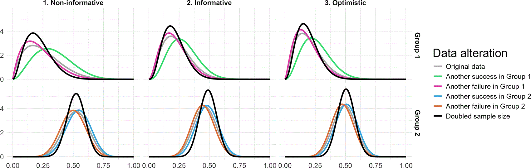
Figure 6. Posterior
distributions of the IBE approach applied to Groups 1 (upper row) and 2 (lower row) for the altered data from the Move Ô case study under each scenario investigated: 1. Non-informative, 2. Informative, 3. Optimistic.
Table 7 reports the effects of data alterations on posterior probabilities
and the Bayes factors
, while Table S10 provides additional information on indicators such as the quantiles of simulated
,
and
, together with 90% HDIs and 90% ETIs. Across all the scenarios investigated, evidence for
over
weakened under unfavourable alterations and strengthened under favourable alterations. The strongest effect was observed when an observation was added to Group 1 because this group was smaller than Group 2. Bayes factors indicated moderate evidence (Non-informative:
; Informative:
; Optimistic:
when adding a success in Group 1) to strong evidence (Non-informative:
; Informative:
; Optimistic:
when adding a failure in Group 1). Doubling the sample size strengthened the indicators in favour of
, with higher posterior probabilities (Non-informative:
; Informative:
; Optimistic:
), larger Bayes factors (Non-informative:
; Informative:
; Optimistic:
), and CIs for
that excluded the null value.
Table 7. Posterior probabilities
and Bayes factors
estimated by the implementation of the IBE approach with our own simulation on the altered data from the Move Ô case study in the three investigated scenarios: 1. Non-informative, 2. Informative, 3. Optimistic.
| | Non-informative
| Informative | Optimistic |
|---|
| Theoretical prior probability
| 0.500 | 0.500 | |
| Another success in Group 1 | Posterior probability
| 0.846 | 0.879 | 0.936 |
| Bayes factor
| 5.467 | 7.176 | 3.667 |
| Another failure in Group 1 | Posterior probability
| 0.952 | 0.954 | 0.981 |
| Bayes factor
| 19.884 | 20.538 | 12.676 |
| Another success in Group 2 | Posterior probability
| 0.938 | 0.950 | 0.977 |
| Bayes factor
| 15.192 | 18.666 | 10.747 |
| Another failure in Group 2 | Posterior probability
| 0.912 | 0.927 | 0.966 |
| Bayes factor
| 10.353 | 12.519 | 7.042 |
| Doubling the sample size | Posterior probability
| 0.984 | 0.987 | 0.994 |
| Bayes factor
| 61.195 | 76.202 | 42.734 |
Influence of data alterations on the results of the LTT approach
Under the LTT approach,
Figure 7 shows that the data alterations affected the simulated distributions of
and
. The largest changes occurred in the
distribution when an additional success was added to Group 1, in both non-informative and informative scenarios. This produced a leftward shift of the distribution, and the use of a truncated positive distribution led to a higher peak. Doubling the sample size also increased the peaks for the parameter distributions.
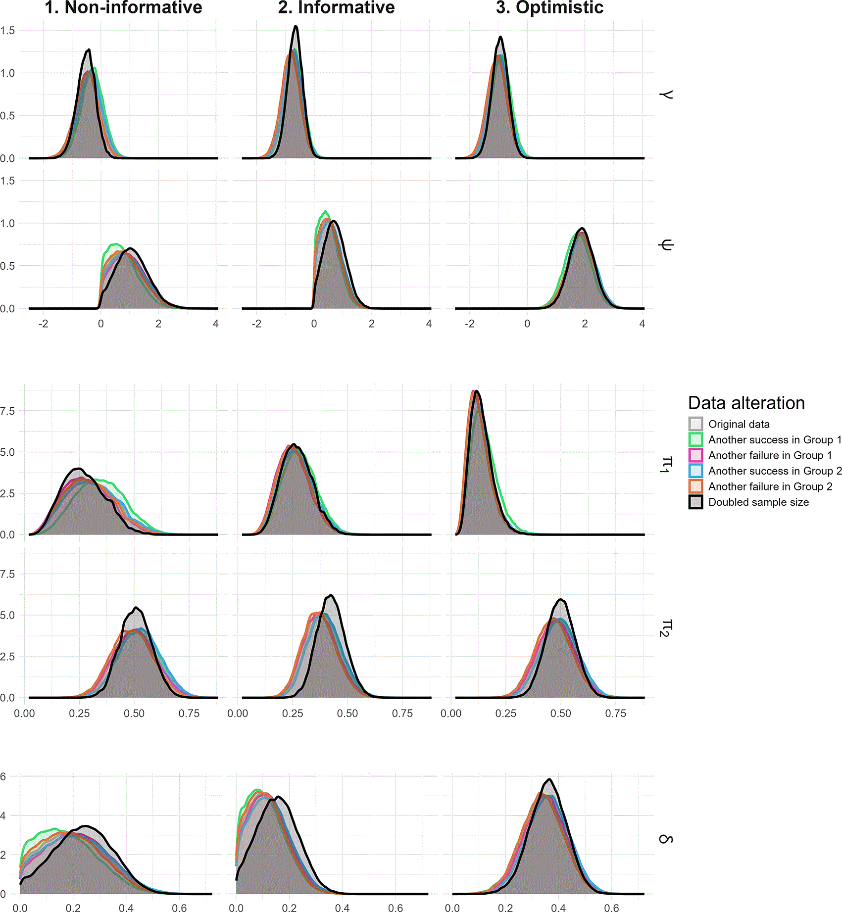
Figure 7. Posterior distributions of the
,
,
and
parameters and the difference
simulated for the altered data from the Move Ô case study by the abtest implementation of the LTT approach for each scenario investigated: 1. Non-informative, 2. Informative, 3. Optimistic.
Although the overall shapes of the
and
distributions remained largely unchanged, the most noticeable alterations were observed for
when the sample size was doubled (
Figure 7). These changes were consistent with expectations. Unfavourable alterations shifted the
distribution to the right and the
distribution to the left. Conversely, favourable alterations shifted the
distribution to the left and the
distribution to the right. Doubling the sample size shifted the
distribution to the right and increased its peak.
As noted above, unfavourable alterations shifted the
distribution to the left, thereby weakening evidence in support of the
hypothesis. By contrast, favourable alterations shifted it to the right, thereby strengthening the evidence for the
hypothesis (
Figure 7). Since the original data supported
, doubling the sample size reinforced this result through a rightward shift and a higher peak.
Table 8 reports the updated posterior probabilities and Bayes factors after the data alterations, together with the hypotheses compared. Table S11 provides supplementary information on the quantiles and CIs of the parameter distributions. The findings were consistent with those obtained under the IBE approach. In all cases, unfavourable alterations (adding a success in Group 1 and a failure in Group 2) reduced the evidence for
over
or
, with Bayes factors indicating weak to moderate evidence for
over
or
(Non-informative: 1.476 to 5.613; Informative: 2.104 to 5.631; Optimistic: 4.019 to 10.921). Favourable alterations (adding a failure in Group 1 and a success in Group 2) strengthened the evidence in favour of
, with Bayes factors indicating weak to strong evidence for
over
or
(Non-informative: 2.497 to 9.321; Informative: 3.075 to 7.303; Optimistic: 14.154 to 19.600). When the sample size was doubled, Bayes factors indicated moderate to very strong evidence for
over
or
(Non-informative: 5.887 and 29.142; Informative: 6.817 and 22.685; Optimistic: 48.706 and 75.390).
Table 8. Prior probabilities, posterior probabilities and Bayes factors estimated by the implementation of the LTT approach with the abtest package to compare
over
and
over
on the altered data from the Move Ô case study in the three investigated scenarios: 1. Non-informative, 2. Informative, 3. Optimistic.
| | | Non-informative
| Informative | Optimistic |
|---|
| Prior probabilities |
over
| Prior probability
| 0.500 | 0.500 | 0.700 |
| Prior probability
| 0.500 | 0.500 | 0.300 |
|
over
| Prior probability
| 0.500 | 0.500 | 0.700 |
| Prior probability
| 0.500 | 0.500 | 0.300 |
| Another success in Group 1 |
over
| Posterior probability
| 0.596 | 0.678 | 0.904 |
| Posterior probability
| 0.404 | 0.322 | 0.096 |
| Bayes factor
| 1.476 | 2.104 | 4.019 |
|
over
| Posterior probability
| 0.791 | 0.811 | 0.922 |
| Posterior probability
| 0.209 | 0.189 | 0.078 |
| Bayes factor
| 3.787 | 4.302 | 5.038 |
| Another failure in Group 1 |
over
| Posterior probability
| 0.740 | 0.755 | 0.971 |
| Posterior probability
| 0.260 | 0.245 | 0.029 |
| Bayes factor
| 2.843 | 3.075 | 14.154 |
|
over
| Posterior probability
| 0.903 | 0.879 | 0.978 |
| Posterior probability
| 0.097 | 0.121 | 0.022 |
| Bayes factor
| 9.321 | 7.276 | 18.884 |
| Another success in Group 2 |
over
| Posterior probability
| 0.714 | 0.756 | 0.972 |
| Posterior probability
| 0.286 | 0.244 | 0.028 |
| Bayes factor
| 2.497 | 3.094 | 14.718 |
|
over
| Posterior probability
| 0.884 | 0.880 | 0.979 |
| Posterior probability
| 0.116 | 0.120 | 0.021 |
| Bayes factor
| 7.632 | 7.303 | 19.600 |
| Another failure in Group 2 |
over
| Posterior probability
| 0.667 | 0.720 | 0.952 |
| Posterior probability
| 0.333 | 0.280 | 0.048 |
| Bayes factor
| 2.002 | 2.569 | 8.459 |
|
over
| Posterior probability
| 0.849 | 0.849 | 0.962 |
| Posterior probability
| 0.151 | 0.151 | 0.038 |
| Bayes factor
| 5.613 | 5.631 | 10.921 |
| Doubling the sample size |
over
| Posterior probability
| 0.855 | 0.872 | 0.991 |
| Posterior probability
| 0.145 | 0.128 | 0.009 |
| Bayes factor
| 5.887 | 6.817 | 48.706 |
|
over
| Posterior probability
| 0.967 | 0.958 | 0.994 |
| Posterior probability
| 0.033 | 0.042 | 0.006 |
| Bayes factor
| 29.142 | 22.685 | 75.390 |
Discussion and conclusion
In this study, we applied both the IBE and LTT approaches to a case study involving an understudied population living in a PICT. Although both approaches were implemented, the literature recommends giving preference to the LTT approach.9 We reviewed, illustrated, and discussed several related indicators in order to assess the possible association between the weight status of children and that of their parents. Even if the present study was not intended as an apologia for the Bayesian framework, it shows that these approaches provide valuable information that deepens the conclusion obtainable from a frequentist test such as Fisher’s exact test, especially when applied to small datasets.40 Rather than ending with a closed conclusion such as “non-significant” or “
rejected”, the analysis makes it possible to distinguish between “evidence of absence”, “absence of evidence”, and even stronger forms of support.8,10 We discuss these points below.
The supplementary materials (Tables S3 to S9 and S12 to S16; Figures S1 to S5) extend the present results with similar findings from another case study conducted on Lifou Island in New Caledonia, another PICT. Although the two case studies addressed similar substantive topic, the two datasets were complementary because of important differences between them. Indeed, the sample size from the Move Ô study was smaller than in the Lifou study (Move Ô:
; Lifou:
), but the estimated difference
was larger in the first case study (Move Ô:
; Lifou:
), as was the effect size
(Move Ô:
; Lifou:
). This explains why the highlighted evidence was weaker in the supplementary case study than in the present one, and why the results were less affected by the data alterations.
This study made it possible to compare the meaning and outputs of the frequentist Fisher’s exact test with those of the Bayesian A/B testing approaches (IBE and LTT). While the frequentist framework focuses on comparing the observed data with the distribution expected under
, the Bayesian framework instead updates both
and the alternative hypothesis, which may be
,
, or
. For the primary dataset considered here, Fisher’s exact test yielded an absence of evidence favouring
over
or
, whereas the Bayes factors calculated from the IBE approach indicated moderate to strong evidence for
over
and the Bayes factors from the LTT approach indicated negligible (i.e. essentially absent) to moderate evidence for
over
8,9 Bayes factors are known to be sensitive to the choice of prior, especially in the small-sample datasets.8,31,40,47 However, we selected three reasonable prior specifications in relation to the present context, and unlike in some previous simulation studies, the substantive conclusions did not change markedly because the Bayes factors never favoured
47
Other indicators, such as the
distribution and the associated 90% CI, as well as the shift from prior to posterior distributions and the corresponding posterior probabilities, provided additional insight. In particular, even when the CI for
included the null value (i.e. in the non-informative and informative scenarios), most of the mass of the
distribution remained above 0, yielding high posterior probabilities in favour of
. These probabilities exceeded 0.90 for the IBE approach; in the LTT approach they ranged from 0.65 to 0.96 when comparing
and
, and exceeded 0.82 when comparing
and
(
Tables 3, 4, S5, and S6). Uncertainty remains, and additional data would strengthen the evidence, but the convergence of these indicators suggests that concluding that
is highly probable is not unreasonable.31
Regarding the data alterations, doubling the sample size was intended to emphasize the effect of sample size on the results and conclusions while leaving the effect size unchanged. The p-values from Fisher’s exact test fell below the conventional rejection threshold (
), and the Bayesian indicators suggested stronger evidence in favour of
over the competing hypotheses. Importantly, the overall shapes of the posterior distributions changed little, except that they became narrower and more peaked. The Bayes-factor evidence for
strengthened to strong to very strong under the IBE approach (
Tables 7 and S15). Under the LTT approach, evidence for
over
was moderate to very strong, whereas evidence for
over
was strong to very strong (
Tables 8 and S16). This type of alteration also illustrates that, when the effect size is larger, increasing the amount of data consistent with the observed effect - in this case, data in favour of
- strengthens the evidence more readily. For example, when the LTT approach was used to compare
and
, Bayes factors for the original data ranged from 2 to 11 in the Move Ô case study (with strong effect size) and from 2 to 3 in the Lifou case study (with moderate effect size) (
Tables 4 and S6); after doubling the sample size, the corresponding ranges were from 6 to 49 and from 5 to 11, respectively (
Tables 8 and S14).
By contrast, adding a single observation led to slight changes in both sample size and effect size. As in the Results section, we distinguish favourable alterations, which provide additional support for
, from unfavourable alterations, which do not. The conclusions based on Fisher’s exact test remained unchanged regardless of the alteration considered (
). The main Bayes-factor conclusions also remained unchanged, although the strength of the evidence for
over competing hypotheses could be slightly increased or decreased depending on the alteration because of the interpretive thresholds used.20,21 It is also noteworthy that, if one estimates the proportion of favourable alterations from the available data, the behaviour of the sampling process should differ between the two case studies. Although this lies beyond the scope of the present paper, stronger evidence can be anticipated in the Move Ô case study (
favourable alterations), whereas it would be weaker in the supplementary Lifou case study (
favourable alterations).
It is important to acknowledge that researchers who are less familiar with the Bayesian framework may find potentially divergent conclusions based on posterior probabilities and Bayes factors frustrating. Etz & Vandekerckhove (2018) clarified the complementary roles of these two indicators.19 Posterior probabilities are useful “to determine our total belief after taking into account the data and to draw conclusions”, whereas Bayes factor serves as “a learning factor that tells us how much evidence the data have delivered”.19 In the case study examined here, no counterintuitive result was observed. The data, along with the resultant high posterior probabilities, were consistent with existing theories and previous case studies.42–44 However, the data provided only limited additional evidence - ranging from negligible to moderate - under the LTT approach, for example.
This paper showed that the application of statistical tools from the Bayesian framework can offer insights that complement those obtained under the conventional frequentist framework. Our aim is not to replace existing practices, but to advocate the inclusion of this additional information in order to obtain a fuller understanding of the situations under study.8 We believe that this approach is particularly valuable for research on understudied populations that are challenging to access. Indeed, interventions in such populations may yield modest yet clinically and developmentally meaningful changes in anthropometric or behavioural outcomes, but these effects are often difficult to demonstrate within the “traditional frequentist framework”.
Consent
We obtained informed written consent from all parents for their participation and their children’s participation before their children entered the study. The research met the legal requirements and the Declaration of Helsinki, and the protocols18,49 were approved by the Consultative Ethics Committee of New Caledonia: CCE 2018–06 01.
Disclosure
Deepl and Paperpal AI assistant were used to improve readability and language of the work and not used to replace researcher tasks such as producing scientific insights, analysing and interpreting data, or drawing scientific conclusions. Human oversight and control have been applied to the text editing improvement, and authors have carefully reviewed and edited the result because AI assistants can generate authoritative-sounding output that can be incorrect, incomplete, or biased.
Supplementary materials
The supplementary materials are included in deposit containing the underlying data.