Active machine learning using MCMC Bayesian neural networks

Devesh Jawla; John Kelleher; Maria Chiara Leva

doi:10.12688/openreseurope.24569.1

Active machine learning using MCMC Bayesian neural networks

Devesh Jawla ,
John Kelleher
,
Maria Chiara Leva

Article

Authors & roles Authors

Peer review record Peer review

Metrics

Cite

Section

Research Article

Published

September 22, 2026

DOI

https://doi.org/10.12688/openreseurope.24569.1

Versions

September 22, 2026 (Published Manuscript Under Review 1.0)

European Commission

Grant ID(s): 955901

Views

Downloads

Citations

See full metrics

Active learning Bayesian neural networks MCMC MCDropout

Abstract

Background

Standard neural networks require large labelled datasets for strong generalization, which is often costly to annotate. Active learning (AL) reduces annotation costs by selecting the most informative samples for labelling based on model uncertainty, and Bayesian methods are a natural source of such uncertainty estimates. Approximate Bayesian methods such as Monte Carlo Dropout (MC Dropout) are scalable but can introduce systematic approximation errors in low-data regimes, whereas Markov Chain Monte Carlo (MCMC) provides higher-fidelity posterior estimates but is typically too computationally expensive for deep learning. We note that MCMC and AL are potentially complementary, since AL is designed to keep the labelled set small, which is exactly the regime in which MCMC is most tractable.

Methods

We investigate whether a small Bayesian neural network trained with MCMC outperforms a larger network using MC Dropout, when both use the same query function, Power Bayesian Active Learning by Disagreement (PowerBALD), across eight tabular classification datasets, an active learning setting with a 100-sample annotation budget, and matched supervised-learning baselines at 100 samples and at full training-set size.

Results

Within the 100-sample annotation budget, the small MCMC-based model achieved higher balanced accuracy than the MC Dropout model in 6 of 8 active learning tasks, and in 4 of 8 tasks in the matched 100-sample supervised setting, with one additional tie. The active learning procedure also matched or exceeded the performance of training on the full dataset in 5 of 8 tasks while using only a small fraction of the annotations.

Conclusions

These results suggest that MCMC is a viable and, in this constrained-budget setting, often preferable alternative to approximate Bayesian inference for active learning, though we do not claim that it is a generally superior inference method outside this low-annotation regime.

Corresponding author

Devesh Jawla

0000-0001-9136-1482

deveshjawla@gmail.com

Grant information

This research is part of the CISC project (Collaborative Intelligence for Safety critical applications) which has received funding from the European Union’s Horizon 2020 Research and Innovation Programme under the Marie Skłodowska‐Curie grant agreement no. 955901

The funders had no role in study design, data collection and analysis, decision to publish, or preparation of the manuscript.

This work is licensed under a Creative Commons Attribution 4.0 International License.

First version published

September 22, 2026 (https://doi.org/10.12688/openreseurope.24569.1)

Latest version published

September 22, 2026 (https://doi.org/10.12688/openreseurope.24569.1)

Introduction

Standard neural networks trained with Stochastic Gradient Descent (SGD) (Robbins and Monro 1951) depend on large labelled datasets to achieve strong generalisation (Mehta et al. 2019). This creates two compounding difficulties: first, obtaining such labels is costly because human domain experts must invest significant time and effort in labelling; second, in many practical settings the underlying data-generating process is itself expensive or slow, so that even unlabelled data may be scarce. Together, these constraints make passive, exhaustive labelling strategies fundamentally unsuitable for data-scarce domains.

Active learning (AL) is a framework that reduces the amount of labelled data required to achieve competitive supervised classification performance by selecting the most informative samples for labelling (Settles 2012; Kumar and Gupta 2020). The informativeness of a candidate sample is typically measured by the model’s uncertainty in classifying it, and Bayesian models are a natural choice (Wilson and Izmailov 2020) for AL because they provide principled uncertainty estimates that decompose into reducible epistemic and irreducible aleatoric components (Depeweg et al. 2018). Directing queries toward regions of high epistemic uncertainty ensures that labelling effort is spent where it reduces the model’s lack of knowledge, rather than where the data is inherently ambiguous.

An AL algorithm consists of two coupled components: a learning algorithm that maintains a probabilistic model of the data, and a query function that scores unlabelled candidates according to how informative their labels would be. At each query step, the query function selects a batch of samples from the unlabelled pool and presents them to an expert annotator; the newly labelled samples are added to the training set and the model is retrained before the next iteration. Uncertainty-based query functions depend on the learning algorithm to supply uncertainty estimates for every pool point, and the quality of those estimates directly determines the quality of the query decisions.

A number of query functions have been proposed in the literature, including Least Confidence (Lewis 1995), Margin Sampling (Settles and Craven 2008), Max Entropy (Cohn et al. 1996), Bayesian Active Learning by Disagreement (BALD) (Houlsby et al. 2011) and its variants Batch Bayesian Active Learning by Disagreement (BatchBALD) (Kirsch et al. 2019) and Power Bayesian Active Learning by Disagreement (PowerBALD) (Kirsch et al. 2023), and Query by Committee (QBC) (Seung et al. 1992), among others. These query functions differ in the type of uncertainty information they consume: Least Confidence and Margin Sampling require only a single predictive probability vector per sample and therefore work with any classifier; QBC requires an ensemble of predictions, and BALD requires an ensemble of probability vectors. PowerBALD, which extends BALD to the batch setting by introducing a stochastic score-based sampling component that promotes diversity, represents the current state of the art for batch Bayesian AL and serves as the primary query function in this study.

The quality of BALD-family query functions depends entirely on the fidelity of the posterior approximation used to generate the ensemble. Standard neural networks trained with Stochastic Gradient Descent (SGD) (Robbins and Monro 1951) produce a single Maximum A Posteriori (MAP) estimate and provide no epistemic uncertainty whatsoever. Approximate Bayesian methods such as Monte Carlo Dropout (MC Dropout) (Gal et al. 2017) and mean-field Variational Inference (VI) (Blundell et al. 2015) are scalable but restrict the posterior to a single optimum, introducing systematic approximation errors that are largest precisely in the low-data regime that characterises every early AL iteration (Wu et al. 2019; Zhao and Ji 2018). Markov Chain Monte Carlo (MCMC), by contrast, provides asymptotically exact posterior samples without restricting the posterior to a parametric family (Neal 1996), making it the gold standard for Bayesian inference and the most reliable source of epistemic uncertainty estimates. However it incurs very high computational costs—scaling with both dataset size and the number of model parameters, and therefore is not commonly used with deep learning.

Therefore, in this paper we argue that the computational constraints of MCMC and the labelling efficiency goal of AL are not in tension but are complementary by design: MCMC is most tractable when the labelled set is small, and AL is explicitly designed to keep the labelled set as small as possible. Restricting the model to a small Bayesian Neural Network (BNN) renders MCMC computationally feasible while preserving the full expressiveness of the posterior. We therefore investigate the following research question:

Does active learning using MCMC in combination with a small BNN outperform active learning using approximate Bayesian inference (MC Dropout) in combination with a larger network, when both approaches use the same state-of-the-art query function PowerBALD?

By holding the query function fixed across both conditions, we isolate the contribution of posterior fidelity combined with small NN to AL performance, providing the first direct empirical test of whether exact posterior inference translates into measurably better query decisions and greater label efficiency in practice.

Methodology

Problem Setting

We consider a standard pool-based active learning setting for supervised classification. Let $L = {(x_{i}, y_{i})}_{i = 1}^{N_{L}}$ denote the labelled set and $U = {x_{j}}_{j = 1}^{N_{U}}$ denote the unlabelled pool, where $N_{L} ≪ N_{U}$ at the start of the AL procedure. At each AL cycle, a query function scores all points in $U$ and selects a batch of $K$ points to be labelled by the oracle; then these points are moved from $U$ to $L$ and the model is retrained on the updated $L$ before the next cycle. The goal is to maximise classification performance on a held-out test set while minimising the total number of oracle queries, i.e. to maximise annotation efficiency.

Learning Algorithms

We compare the active learning performance of two learning algorithms that differ in both inference method and network size, chosen to test the central hypothesis that MCMC with a small BNN is a feasible and competitive alternative to approximate Bayesian inference with a larger network.

MCMC with a Small Bayesian Neural Network

The first configuration uses a small BNN with one hidden layer trained via MCMC using the No-U-Turn Sampler (NUTS) (Hoffman and Gelman 2011), a state-of-the-art adaptive variant of Hamiltonian Monte Carlo (HMC) (Neal 1996). The prior on all weights and biases is a layer wise scaled Gaussian: $θ_{n} \sim N (0, σ_{n}^{2})$ , where $σ_{n}^{2}$ is scaled according to the width of layer $n$ (Jawla and Kelleher 2025). Rather than producing a single point estimate of the weights, NUTS draws $S$ samples ${θ^{(s)}}_{s = 1}^{S}$ from the posterior distribution $p (θ | L)$ , yielding a posterior ensemble of $S$ distinct networks. Predictions are formed by averaging over this ensemble to approximate the posterior predictive integral:

p (y | x, L) = \int p (y | x, θ) p (θ | L) d θ \approx \frac{1}{S} \sum_{s = 1}^{S} p (y | x, θ^{(s)}) .

The posterior ensemble provides asymptotically exact epistemic uncertainty estimates without restricting the posterior to a parametric family—unlike Variational Inference, MC dropout or Laplace Approximation, making it the most faithful source of uncertainty information available for the query function. We run 8 parallel chains and sample 1000 Monte Carlo steps after the burn-in period. Every fourth sample is retained per chain, yielding an ensemble of 2000 approximately uncorrelated networks.

The network architecture (see Figure 1 for the architecture) is a single hidden layer of four neurons: all categorical input features feed into one shared neuron, and all continuous input features feed into the remaining three shared neurons, with ReLU activations throughout and no bias on the output layer. We developed this architecture to represent the class of small Bayesian neural networks. Our initial tests showed it gave reasonably good performance. Although we are not claiming that this is the only optimal architecture. This architecture is deliberately small to keep the MCMC parameter space tractable. While prior work applying HMC to neural networks typically uses 2–3 hidden layers with 10–50 neurons (Depeweg et al. 2018; Wenzel et al. 2020; Noci et al. 2021; Izmailov et al. 2021; Olivier et al. 2021), none of these studies use a network as small as ours, with a single hidden layer of only four neurons. We use a class-weighted likelihood (Jawla and Kelleher 2025), rather than correcting for class imbalance through under- or over-sampling.

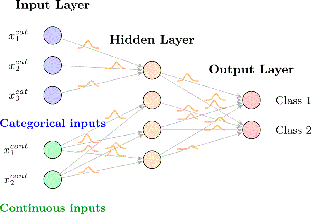
Figure 1. Architecture of our small Bayesian neural network.

MC Dropout with a Deep Neural Network

The second configuration uses a larger network with three hidden layers of 100 neurons each, trained using SGD, and then MC Dropout (Gal et al. 2017) is used as an approximate Bayesian inference method for uncertainty quantification. This configuration is the primary AL baseline, representative of the standard approach in the deep Bayesian AL literature (Gal et al. 2017; Siddhant and Lipton 2018). Dropout is retained at test time and $S$ stochastic forward passes are performed for each input, producing an approximate posterior ensemble analogous to that of the MCMC configuration. Predictions and uncertainty estimates are obtained by averaging over these stochastic passes:

p (y | x, L) \approx \frac{1}{S} \sum_{s = 1}^{S} p (y | x, {\hat{θ}}^{(s)}),

where

{\hat{θ}}^{(s)}

denotes the network weights with a dropout mask applied at the

s

-th forward pass. MC Dropout is computationally efficient and widely used in the deep AL literature (Gal et al. 2017; Siddhant and Lipton 2018), but restricts the posterior to a single optimum that systematically underestimates posterior variance, particularly in the low-data regime (Zhao and Ji 2018). The larger network size reflects the standard practice in deep AL, where model capacity is increased to compensate for the approximation error of the inference method.

Query function

Both AL configurations use PowerBALD (Kirsch et al. 2023) as the query function. PowerBALD extends BALD (Houlsby et al. 2011) to the batch setting by replacing deterministic top- $K$ selection with stochastic sampling proportional to a power of the BALD score, promoting diversity within the acquired batch at negligible additional computational cost. The BALD score for a candidate point $x$ is:

BALD (x) = ℍ [y | x, L] - E_{p (θ | L)} [ℍ [y | x, θ]],

where the first term is the total predictive entropy and the second is the expected entropy under the posterior, i.e. the aleatoric uncertainty. BALD therefore targets epistemic uncertainty specifically, and its quality as a query function depends directly on how faithfully the posterior ensemble approximates the true posterior. By holding the query function fixed across both AL configurations, we ensure that any observed difference in AL performance is attributable solely to the inference method and network size rather than the query function.

Formally, PowerBALD (Kirsch et al. 2023) is defined by modelling as a perturbation of the log-score with Gumbel-distributed noise:

BAL D_{power} (x) ≔ log BALD (x) + ϵ, ϵ \sim Gumbel (0, 1 / β)

where we select the top-

K

samples by

BAL D_{power}

Experimental protocol

We perform three sets of experiments to answer two questions: what is the upper bound on classification performance achievable by any of the models on each dataset, and which combination of inference method and network size achieves the best annotation efficiency in the active learning setting.

1. Active learning. The unlabelled pool at each AL run consists of the full training set of the corresponding 10-fold split. At each query step, $K = 10$ samples are selected by PowerBALD for annotation, for a total of 10 query steps, giving a maximum labelling budget of 100 samples per fold. Classification performance on the held-out test set is reported after each query step to show the learning curve across the AL cycle.
2. Supervised learning with all available training samples. As the computational cost of running MCMC on large data sets is prohibitive, we only let the Deep NN train on the full training set of each 10-fold split and evaluated on the corresponding test set with MC dropout applied at test time to obtain robust predictions. This establishes the upper bound on classification performance achievable given completely annotated train set.
3. Supervised learning with 100 randomly selected training samples. Both models participate in this experiment, and each model is trained on the same 100 randomly drawn samples from the training set of each 10-fold split. This serves two purposes: it isolates the contribution of the inference method from the contribution of the query function, and it provides a low-data supervised baseline directly comparable to the active learning results at the final query step.

Comparing each AL configuration against the corresponding 100-sample supervised baseline quantifies the benefit of active learning: a large gap indicates that the query function is making efficient use of the labelling budget, while a small gap indicates that random selection is already sufficient and the choice of query function has limited impact. Comparing both AL configurations against the full supervised baseline establishes how closely active learning with a limited budget recovers the performance of training on all available data.

More information about the datasets, data-preprocessing, evaluation metrics, and implementation can be found in Section 6 (Experiment Details).

Results

For the three experiments we obtain the results as follows:

The experimental results summarized in Table 1 demonstrate that the Small BNN (MCMC) approach is the most effective model across the majority of the evaluated tasks, achieving the highest balanced accuracy on 6 out of the 8 datasets.

Table 1. Active learning classification performance.

Data set	Model (Algorithm)	Annotations	Bal. Acc.
Coalmine	Deep NN (MC Dropout)	80	51.2 ± 1.3
	Small BNN (MCMC)	90	62.8 ± 5.5
Stroke	Deep NN (MC Dropout)	20	51.8 ± 2.3
	Small BNN (MCMC)	80	61.9 ± 3.9
Banknote	Deep NN (MC Dropout)	50	100.0 ± 0.0
	Small BNN (MCMC)	50	97.2 ± 0.4
Iris	Deep NN (MC Dropout)	30	90.0 ± 12.3
	Small BNN (MCMC)	30	93.6 ± 5.3
Yeast	Deep NN (MC Dropout)	80	46.7 ± 12.2
	Small BNN (MCMC)	100	31.1 ± 4.9
Adult	Deep NN (MC Dropout)	100	67.6 ± 1.4
	Small BNN (MCMC)	80	75.7 ± 0.6
C. Default	Deep NN (MC Dropout)	90	57.4 ± 1.3
	Small BNN (MCMC)	90	57.5 ± 2.1
C. Fraud	Deep NN (MC Dropout)	100	50.0 ± 0.0
	Small BNN (MCMC)	100	52.6 ± 3.2

The supervised learning benchmarks, detailed in Tables 2 and 3, 4 illustrate the impact of training data volume on predictive performance. When utilizing the full training set, the MC Dropout achieves high balanced accuracies in datasets like C. Default, C. Fraud and Adult. However, when the training budget is restricted to 100 samples, there is a notable shift in the optimal algorithm; the Small NN (MCMC) becomes the top performer for five of the datasets, suggesting better generalization in low-data regimes. There is also a significant degradation in C. Default, and C. Fraud datasets when moving from full supervised learning to a 100-sample supervised learning.

Table 2. MC Dropout Deep NN’s supervised learning performance with all available samples in the training set.

Data set	Train size	Bal. Acc.	Time (s)
Coalmine	2326	60.2 ± 4.8	31.0 ± 7.4
Stroke	4599	62.0 ± 2.4	69.1 ± 12.9
Banknote	1235	100.0 ± 0.0	4.1 ± 1.0
Iris	135	96.9 ± 4.3	2.0 ± 0.3
Yeast	1336	57.1 ± 5.2	13.5 ± 2.2
Adult	43958	82.5 ± 0.3	295.1 ± 37.8
C. Default	27000	70.7 ± 1.4	230.9 ± 61.4
C. Fraud	256327	93.4 ± 1.4	1213.9 ± 381.6

Table 3. Supervised learning performance with 100 training samples.

Data set	Model (Algorithm)	Bal. Acc.
Coalmine	Deep NN (MC Dropout)	53.5 ± 2.6
	Small BNN (MCMC)	59.8 ± 4.0
Stroke	Deep NN (MC Dropout)	51.7 ± 1.8
	Small BNN (MCMC)	55.7 ± 3.4
Banknote	Deep NN (MC Dropout)	99.4 ± 0.6
	Small BNN (MCMC)	97.8 ± 0.9
Iris	Deep NN (MC Dropout)	97.2 ± 2.3
	Small BNN (MCMC)	97.2 ± 5.4
Yeast	Deep NN (MC Dropout)	48.5 ± 6.4
	Small BNN (MCMC)	36.6 ± 8.0
Adult	Deep NN (MC Dropout)	65.8 ± 1.6
	Small BNN (MCMC)	75.9 ± 0.5
C. Default	Deep NN (MC Dropout)	60.5 ± 1.4
	Small BNN (MCMC)	63.0 ± 1.1
C. Fraud	Deep NN (MC Dropout)	52.9 ± 5.7
	Small BNN (MCMC)	51.9 ± 3.7

Table 4. Query sizes, train sizes and class imbalance of the eight real data sets.

Data set	% Minority class	Folds	Query size	Total queries	Total samples
Adult	0.22	10	10	10	48720
Banknote	0.44	10	10	10	1377
Credit Fraud	0.17	10	10	10	284767
Credit Default	0.22	10	10	10	29920
Coalmine	0.06	10	10	10	2584
Stroke	0.05	10	10	10	4916
Iris	0.3	5	6	5	150
Yeast	0.003	10	10	10	1496

The comparison between Active Learning (AL) and Supervised Learning (SL) baselines, illustrated in Figure 2, highlights the efficiency of the AL approach across multiple datasets. Based on the maximum values achieved over 10 standard folds with $95 %$ confidence intervals, AL demonstrates a clear advantage over SL with a restricted budget of 100 randomly annotated samples in 3 out of 8 datasets. Furthermore, the AL framework proves to be highly competitive with SL using the full training set on 5 out of 8 datasets, where competitiveness is defined by the overlap of confidence intervals.

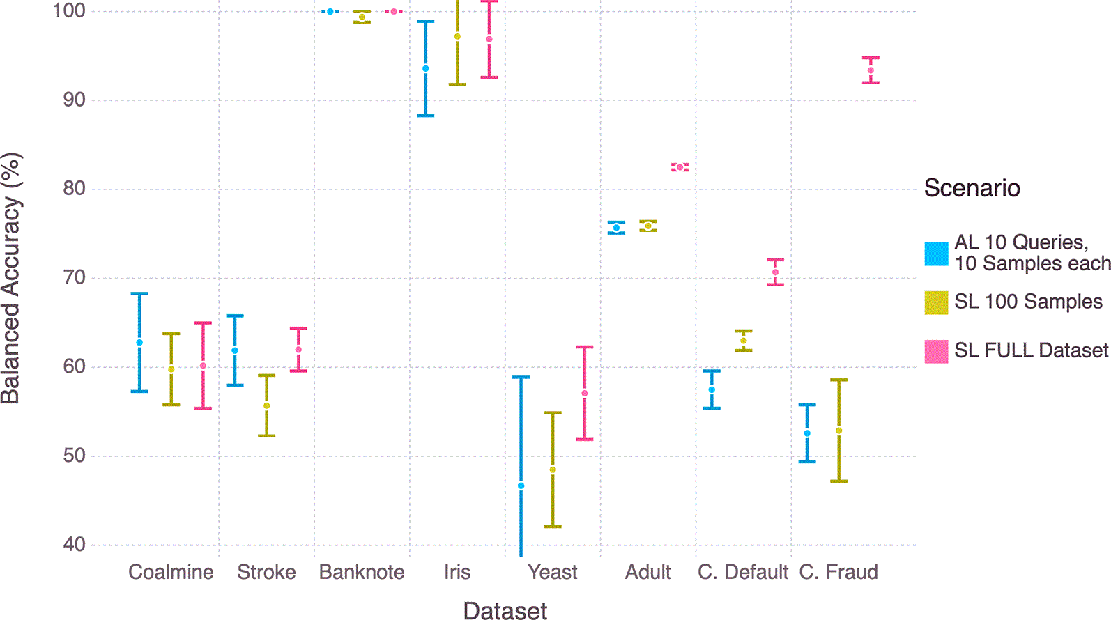
Figure 2. Best results in Active learning (AL) with maximum of 10 query steps (max 100 samples), Supervised Learning with 100 samples, and Supervised Learning (SL) with all samples.

Discussion

The experimental results presented in Tables 1 through 3 provide several key insights into the behavior of Bayesian neural networks in data-constrained environments.

A primary observation is the superiority of the Small BNN (MCMC) approach in active learning. As shown in Table 1, this model achieved the highest balanced accuracy in 6 out of 8 active learning tasks. This trend persists in supervised learning benchmarks with limited budgets (100 samples), where the MCMC-based model outperformed MC Dropout in five out of eight datasets. This is due to the fact that the Markov Chain Monte Carlo method provides a more reliable posterior approximation when labels are scarce, whereas the MC Dropout approximation requires significantly larger training sets to achieve competitive generalization.

Finally, the comparison between Active Learning (AL) and Supervised Learning (SL) baselines underscores the efficiency of the AL framework. The fact that AL reached performance levels competitive with the full supervised training set in five out of eight datasets—using only a fraction of the total annotations—is a testament to the value of uncertainty-based sample selection. By identifying and labelling only the most informative points, the AL approach effectively bridges the gap between low-budget constraints and high-accuracy requirements.

Limitations. Our comparison varies both the inference method and the network size simultaneously, so the observed gap cannot be decomposed into the contribution of MCMC versus the contribution of a smaller architecture. A natural ablation would be to apply MC Dropout to the small BNN itself, isolating the effect of the inference method under a fixed architecture. We did not run this ablation because our small BNN architecture is not well suited to dropout: its hidden layer has only four neurons in total ( Figure 1)—one shared neuron receiving all categorical features and three shared neurons receiving all continuous features—so masking units at typical dropout rates removes a large fraction of the layer’s already minimal capacity, and leaves too few units for the Bernoulli mask to generate a meaningfully diverse ensemble. Applying MC Dropout to a small BNN in a way that produces a fair comparison would likely require redesigning the architecture around dropout’s requirements, which conflicts with our goal of keeping the architecture chosen for MCMC tractability constant across the comparison. Disentangling the inference method from the architecture, for example by applying MCMC to the larger network or by designing a dropout-compatible small architecture, is left to future work.

Conclusion

This paper does not claim that MCMC is a generally better inference method than MC Dropout for deep learning. Rather, our contribution is to show that MCMC and active learning are complementary by design: AL exists precisely to keep the labelled set small, and a small labelled set is exactly the regime in which MCMC is computationally tractable. We tested whether this complementarity pays off by pairing MCMC with a small BNN against MC Dropout with a larger network under a matched query function (PowerBALD), and evaluating them within the annotation budgets that AL is meant to operate in.

Within the 100-sample annotation budget explored in this paper, our findings lead to the following conclusions:

• Under active learning with a 100-sample annotation budget, the Small BNN using MCMC achieved the highest balanced accuracy in 6 out of 8 datasets ( Table 1), and in the equivalent 100-sample supervised setting it outperformed MC Dropout on 4 out of 8 datasets, tied on 1 (Iris), and underperformed on 3 ( Table 3). This indicates that, in the low-annotation-budget regime targeted by AL, MCMC’s higher-fidelity posterior more often translates into better query decisions and better generalisation than MC Dropout’s approximate posterior.
• Deep networks utilizing MC Dropout are highly dependent on large training volumes, and their performance degrades significantly in restricted-budget environments, seen particularly in the case of the Coalmine, Adult and Credit Default datasets.
• The active learning framework proved to be highly data-efficient, matching or exceeding the performance of models trained on the entire dataset in 5 out of 8 datasets while requiring only a small fraction of the annotations.

Taken together, these results support our central claim: within the annotation budgets where AL operates, MCMC is not merely feasible but competitive with, and frequently superior to, the standard MC Dropout approach, despite using orders of magnitude fewer parameters ( Table 5). We make no claim about which method is preferable once annotation budgets are large or unconstrained, a regime in which MCMC’s computational cost remains prohibitive and MC Dropout’s advantages, as shown in Table 2, dominate. We also note that our comparison changes network size alongside inference method, so the reported gap reflects the combined effect of both factors rather than the inference method in isolation; as discussed above, applying MC Dropout to our small BNN architecture is not well posed given its minimal hidden-layer width, and disentangling the two factors is left to future work.

Table 5. Number of parameters for different models.

Data set	Model (Algorithm)	No. of Parameters
Coalmine	Deep NN (MC Dropout)	22400
	Small NN (MCMC)	59
Adult	Deep NN (MC Dropout)	25500
	Small NN (MCMC)	89
Credit Default	Deep NN (MC Dropout)	23700
	Small NN (MCMC)	90
Stroke	Deep NN (MC Dropout)	22400
	Small NN (MCMC)	53
Bank note	Deep NN (MC Dropout)	20900
	Small NN (MCMC)	21
Credit Fraud	Deep NN (MC Dropout)	23300
	Small NN (MCMC)	93
Iris	Deep NN (MC Dropout)	21000
	Small NN (MCMC)	24
Yeast	Deep NN (MC Dropout)	22100
	Small NN (MCMC)	57

Future work could explore the integration of more sophisticated acquisition functions within the MCMC framework to further enhance the efficiency of the active learning process in high-dimensional datasets. Future work could also explore MC Dropout on a small architecture designed to be dropout-compatible, or MCMC applied to a larger network, to isolate the contribution of inference method from network size.

Ethics and consent

Ethical approval and consent were not required

Experiment details

Datasets

We evaluate on eight tabular datasets of varying size, class balance, and feature types (Categorical, Binary, Continuous, Cardinal, Integers), selected to reflect the resource-intensive nature of MCMC inference: Adult (Becker and Kohavi 1996), Fake Banknote Detection (Lohweg 2013), Credit Fraud Detection (Dal Pozzolo et al. 2017), Stroke Detection (Kansadub et al. 2015), Credit Default Detection (Yeh 2016), Coalmine Bumps Detection (Sikora and Wrobel 2010), Iris Classification (Fisher 1988), and Yeast Classification (Nakai 1996). All datasets are split using standard 10-fold train:test splits.

Data pre-processing

We perform minimal pre-processing, removing only redundant features, rows with missing values, and NaN values. Continuous features are scaled according to their distributional properties: MinMax scaling is applied to features with known domain boundaries, MaxAbs scaling (division by the feature maximum) is applied to sparse features, and standardisation (zero mean, unit variance) is applied to normally distributed continuous features that fall into neither of the previous categories. Categorical features are encoded using one-hot encoding throughout.

Implementation

All models are implemented using Flux.jl (Innes 2018). Bayesian models are defined using Turing.jl (Ge et al. 2018), which internally computes the log joint probability at each sample via the @model macro, so that the user need only specify the prior and likelihood and choose an MCMC sampler. For SGD-trained Deep NN, we use the AdaBelief optimiser (Zhuang et al. 2020) for 500 epochs with L2 regularisation (decay $= 0.01$ ), learning rate 0.001, and early stopping, saving the best model. The batch size for the full trainig sets was 512, for data sizes less than 512, for example in the active elarning experiements all the samples were used in a single batch for training.

MC Dropout rate was set at 20%.

Depending on the data set, and the learning algorithm, we have a different number of learnable parameters (see Table 5)

Evaluation metrics

To benchmark the classification performance we use Balanced Accuracy for all the data sets, and F1Score for the Binary tasks, and Average Class Accuracy Harmonic Mean (Kelleher et al. 2020) for the multi class tasks.

And to benchmark the efficiency of the models we measure the time required to sample the total number of MC samples.

To test for convergence of the chains, we look at the following metrics:

1. Gelman Diagnostic (Vehtari et al. 2019) - Convergence statistic which tells us how well the chains have mixed, it compares the between- and within-chain estimates for weights and biases.
2. Avg ESS (effective sample size) (Geyer 1992) - it is an indication of the number of independent samples contained in a chain

Data availability

Six of the eight datasets used in this study are hosted on the UCI Machine Learning Repository (https://archive.ics.uci.edu), each released under a CC-BY 4.0 license:

Adult (Becker and Kohavi 1996): census records used to predict whether an individual's income exceeds a threshold, based on demographic and employment attributes. DOI: 10.24432/C5XW20.

Banknote Authentication (Lohweg 2013): wavelet-transformed features extracted from images of genuine and forged banknotes, used to predict authenticity. DOI: 10.24432/C55P57.

Default of Credit Card Clients (Yeh 2016): demographic and repayment-history records of credit card clients in Taiwan, used to predict default on payment. DOI: 10.24432/C55S3H.

Iris (Fisher 1988): sepal and petal measurements of three Iris species, used for multi-class species classification. DOI: 10.24432/C56C76.

Yeast (Nakai 1996): protein sequence-derived features used to predict cellular localization sites. DOI: 10.24432/C5KG68.

Seismic Bumps, referred to as Coalmine in this paper (Sikora and Wrobel 2010): sensor readings from a coal mine's seismic hazard monitoring system, used to predict hazardous seismic bump events. DOI: 10.24432/C5W902.

The remaining two datasets are hosted on Kaggle (https://www.kaggle.com):

Credit Card Fraud Detection (Dal Pozzolo et al. 2017): anonymized transaction records from European cardholders, used to predict fraudulent transactions. https://www.kaggle.com/datasets/mlg-ulb/creditcardfraud. This dataset is released under the Database Contents License (DbCL) v1.0, an Open Data Commons attribution license comparable in effect to CC-BY 4.0.

Stroke Prediction Dataset (Fedesoriano, n.d.): demographic and health attributes used to predict stroke occurrence. https://www.kaggle.com/datasets/fedesoriano/stroke-prediction-dataset. The dataset page states “Data files © Original Authors” and, under Acknowledgements, describes the underlying source as confidential and restricts use to educational purposes. It does not name an open license and does not meet a CC0, CC-BY 4.0, or equivalent standard. This dataset uses a demographic and health feature set similar to that used by Kansadub et al. (2015) for stroke risk prediction, though the underlying data is distinct.

Bibliography

Blundell C, Cornebise J, Kavukcuoglu K, et al.: Weight Uncertainty in Neural Network. International Conference on Machine Learning. 2015; 1613–1622.
Cohn DA, Ghahramani Z, Jordan MI: Active Learning with Statistical Models. J. Artif. Intell. Res. 1996; 4: 129–145. Publisher Full Text
Pozzolo D, Andrea GB, Caelen O, et al.: Credit Card Fraud Detection: A Realistic Modeling and a Novel Learning Strategy. IEEE Trans. Neural Networks Learn. Syst. 2017; 29(8): 3784–3797.
Depeweg S, Hernandez-Lobato J-M, Doshi-Velez F, et al.: Decomposition of Uncertainty in Bayesian Deep Learning for Efficient and Risk-Sensitive Learning. Proceedings of the 35th International Conference on Machine Learning, Proceedings of machine learning research. 2018; vol. 80: 1184–93.
Gal Y, Islam R, Ghahramani Z. Deep Bayesian Active Learning with Image Data. Proceedings of the 34th International Conference on Machine Learning. Precup D, Teh YW, editors. Proceedings of Machine Learning Research. PMLR; 2017; vol. 70. .
Ge H, Xu K, Ghahramani Z. Turing: A Language for Flexible Probabilistic Inference. Proceedings of Machine Learning Research. 2018. ahead of print. Publisher Full Text
Geyer CJ: Practical Markov Chain Monte Carlo. Stat. Sci. 1992; 7: 473–483. Publisher Full Text
Hoffman M, Gelman A: The No-u-Turn Sampler: Adaptively Setting Path Lengths in Hamiltonian Monte Carlo. Journal of Machine Learning Research. 2011. ahead of print. Publisher Full Text
Houlsby N, Huszár F, Ghahramani Z, et al.: Bayesian Active Learning for Classification and Preference Learning. Stat. 2011; 1050: 24.
Innes M: Flux: Elegant Machine Learning with Julia. J. Open Source Softw. 2018. ahead of print. Publisher Full Text
Izmailov P, Vikram S, Hoffman MD, et al.: What Are Bayesian Neural Network Posteriors Really Like?. PMLR; 2021.
Jawla D, Kelleher J: Layer Wise Scaled Gaussian Priors for Markov Chain Monte Carlo Sampled Deep Bayesian Neural Networks. Frontiers in Artificial Intelligence. 2025; 8: 1444891. PubMed Abstract | Publisher Full Text | Free Full Text
Kansadub T, Thammaboosadee S, Kiattisin S, et al.: Stroke Risk Prediction Model Based on Demographic Data. Biomedical Engineering International Conference. 2015. ahead of print. Publisher Full Text
Kelleher JD, Namee BM, D’arcy A: Fundamentals of Machine Learning for Predictive Data Analytics: Algorithms, Worked Examples, and Case Studies. MIT press; 2020.
Kirsch A, van Amersfoort J , Gal Y: BatchBALD: Efficient and Diverse Batch Acquisition for Deep Bayesian Active Learning. Adv. Neural Inf. Proces. Syst. 2019; 32(NeurIPS 2019): 7024–7035.
Kirsch A, Farquhar S, Atighehchian P, et al.: Stochastic Batch Acquisition: A Simple Baseline for Deep Active Learning. Transactions on Machine Learning Research. 2023.
Kumar P, Gupta A: Active Learning Query Strategies for Classification, Regression, and Clustering: A Survey. J. Comput. Sci. Technol. 2020; 35(4): 913–945. Publisher Full Text
Lewis DD: A Sequential Algorithm for Training Text Classifiers: Corrigendum and Additional Data. Acm Sigir Forum. 1995; 29: 13–19. Publisher Full Text
Mehta P, Bukov M, Wang C-H, et al.: A High-Bias, Low-Variance Introduction to Machine Learning for Physicists. Phys. Rep. 2019; 810: 1–124. PubMed Abstract | Publisher Full Text | Free Full Text
Neal RM: Bayesian Learning for Neural Networks. Lecture Notes in Statistics. 1996; 118. Publisher Full Text
Noci L, Roth K, Bachmann G, et al.: Disentangling the Roles of Curation, Data-Augmentation and the Prior in the Cold Posterior Effect. Adv. Neural Inf. Proces. Syst. 2021; 34: 12738–12748.
Olivier A, Shields MD, Graham-Brady L: Bayesian Neural Networks for Uncertainty Quantification in Data-Driven Materials Modeling. Comput. Methods Appl. Mech. Eng. 2021; 386: 114079. Publisher Full Text
Robbins H, Monro S: A Stochastic Approximation Method. Ann. Math. Stat. 1951; 22: 400–407. Publisher Full Text
Settles B: Active Learning. Morgan: Claypool Publishers; 2012.
Settles B, Craven M: An Analysis of Active Learning Strategies for Sequence Labelling Tasks. Proceedings of the 2008 Conference on Empirical Methods in Natural Language Processing. 2008; 1070–79.
Seung HS, Opper M, Sompolinsky H: Query by Committee. Proceedings of the Fifth Annual Workshop on Computational Learning Theory. 1992; 287–94.
Siddhant A, Lipton ZC: Deep Bayesian Active Learning for Natural Language Processing: Results of a Large-Scale Empirical Study. Proceedings of the 2018 Conference on Empirical Methods in Natural Language Processing. 2018; 2904–9.
Sikora M, Wrobel L: Application of Rule Induction Algorithms for Analysis of Data Collected by Seismic Hazard Monitoring Systems in Coal Mines. Arch. Min. Sci. 2010; 55(1): 91–114.
Vehtari A, Gelman A, Simpson D, et al.: Rank-Normalization, Folding, and Localization: An Improved R̂ for Assessing Convergence of MCMC. Bayesian Anal. 2019; 16(2). Publisher Full Text
Wenzel F, Roth K, Veeling B, et al.: How Good Is the Bayes Posterior in Deep Neural Networks Really?. International Conference on Machine Learning. 2020; 10248–59.
Wilson AG, Izmailov P: Bayesian Deep Learning and a Probabilistic Perspective of Generalization. Adv. Neural Inf. Proces. Syst. 2020; 33: 4697–4708.
Wu A, Nowozin S, Meeds E, et al.: Deterministic Variational Inference for Robust Bayesian Neural Networks. International Conference on Learning Representations (ICLR). 2019.
Zhao R, Ji Q: An Empirical Evaluation of Bayesian Inference Methods for Bayesian Neural Networks. Proceedings of the British Machine Vision Conference (BMVC). 2018.
Becker B, Kohavi R: Adult. Adult Dataset. UCI Machine Learning Repository; 1996.
Fisher RA: Iris. Iris Dataset. UCI Machine Learning Repository; 1988.
Yeh I-C: default of credit card clients. Credit Fraud Dataset. UCI Machine Learning Repository; 2016.
Nakai K: Yeast. Yeast Dataset. UCI Machine Learning Repository; 1996.
Lohweg V: Banknote Authentication. Banknote Dataset. 2013.
Zhuang J, Tang T, Ding Y, et al.: Adabelief Optimizer: Adapting Stepsizes by the Belief in Observed Gradients. Adv. Neural Inf. Proces. Syst. 2020; 33: 18795–18806.

Comments

Publication information

Section

Research Article

Published

September 22, 2026

DOI

https://doi.org/10.12688/openreseurope.24569.1

Versions

September 22, 2026 (Published Manuscript Under Review 1.0)

Included in

Funding data

European Commission

Grant ID(s): 955901

Metrics

Views

Downloads

Citations

See full metrics

Keywords

Active learning Bayesian neural networks MCMC MCDropout

Comments

Devesh Jawla

School of Computer Science, Technological University Dublin, Dublin, Leinster, Ireland

Roles

Corresponding Author, Co-Author, Conceptualization, Data Curation, Formal Analysis, Investigation, Methodology, Validation, Visualization, Writing – Original Draft Preparation, Writing – Review & Editing

0000-0001-9136-1482

deveshjawla@gmail.com

John Kelleher

School of Computer Science, Technological University Dublin, Dublin, Leinster, Ireland

Roles

Co-Author, Methodology, Project Administration, Resources, Supervision, Validation, Writing – Review & Editing

john.kelleher@tcd.ie

Maria Chiara Leva

School of Computer Science, Technological University Dublin, Dublin, Leinster, Ireland

Roles

Co-Author, Funding Acquisition, Project Administration, Supervision

mariachiara.leva@TUDublin.ie

Downloads over the last 12 months:

Cited by

via Crossref

View citing articles

[1] Blundell C, Cornebise J, Kavukcuoglu K, et al.: Weight Uncertainty in Neural Network. International Conference on Machine Learning. 2015; 1613–1622.

[2] Cohn DA, Ghahramani Z, Jordan MI: Active Learning with Statistical Models. J. Artif. Intell. Res. 1996; 4: 129–145. Publisher Full Text

[3] Pozzolo D, Andrea GB, Caelen O, et al.: Credit Card Fraud Detection: A Realistic Modeling and a Novel Learning Strategy. IEEE Trans. Neural Networks Learn. Syst. 2017; 29(8): 3784–3797.

[4] Depeweg S, Hernandez-Lobato J-M, Doshi-Velez F, et al.: Decomposition of Uncertainty in Bayesian Deep Learning for Efficient and Risk-Sensitive Learning. Proceedings of the 35th International Conference on Machine Learning, Proceedings of machine learning research. 2018; vol. 80: 1184–93.

[5] Gal Y, Islam R, Ghahramani Z. Deep Bayesian Active Learning with Image Data. Proceedings of the 34th International Conference on Machine Learning. Precup D, Teh YW, editors. Proceedings of Machine Learning Research. PMLR; 2017; vol. 70. .

[6] Ge H, Xu K, Ghahramani Z. Turing: A Language for Flexible Probabilistic Inference. Proceedings of Machine Learning Research. 2018. ahead of print. Publisher Full Text

[7] Geyer CJ: Practical Markov Chain Monte Carlo. Stat. Sci. 1992; 7: 473–483. Publisher Full Text

[8] Hoffman M, Gelman A: The No-u-Turn Sampler: Adaptively Setting Path Lengths in Hamiltonian Monte Carlo. Journal of Machine Learning Research. 2011. ahead of print. Publisher Full Text

[9] Houlsby N, Huszár F, Ghahramani Z, et al.: Bayesian Active Learning for Classification and Preference Learning. Stat. 2011; 1050: 24.

[10] Innes M: Flux: Elegant Machine Learning with Julia. J. Open Source Softw. 2018. ahead of print. Publisher Full Text

[11] Izmailov P, Vikram S, Hoffman MD, et al.: What Are Bayesian Neural Network Posteriors Really Like?. PMLR; 2021.

[12] Jawla D, Kelleher J: Layer Wise Scaled Gaussian Priors for Markov Chain Monte Carlo Sampled Deep Bayesian Neural Networks. Frontiers in Artificial Intelligence. 2025; 8: 1444891. PubMed Abstract | Publisher Full Text | Free Full Text

[13] Kansadub T, Thammaboosadee S, Kiattisin S, et al.: Stroke Risk Prediction Model Based on Demographic Data. Biomedical Engineering International Conference. 2015. ahead of print. Publisher Full Text

[14] Kelleher JD, Namee BM, D’arcy A: Fundamentals of Machine Learning for Predictive Data Analytics: Algorithms, Worked Examples, and Case Studies. MIT press; 2020.

[15] Kirsch A, van Amersfoort J , Gal Y: BatchBALD: Efficient and Diverse Batch Acquisition for Deep Bayesian Active Learning. Adv. Neural Inf. Proces. Syst. 2019; 32(NeurIPS 2019): 7024–7035.

[16] Kirsch A, Farquhar S, Atighehchian P, et al.: Stochastic Batch Acquisition: A Simple Baseline for Deep Active Learning. Transactions on Machine Learning Research. 2023.

[17] Kumar P, Gupta A: Active Learning Query Strategies for Classification, Regression, and Clustering: A Survey. J. Comput. Sci. Technol. 2020; 35(4): 913–945. Publisher Full Text

[18] Lewis DD: A Sequential Algorithm for Training Text Classifiers: Corrigendum and Additional Data. Acm Sigir Forum. 1995; 29: 13–19. Publisher Full Text

[19] Mehta P, Bukov M, Wang C-H, et al.: A High-Bias, Low-Variance Introduction to Machine Learning for Physicists. Phys. Rep. 2019; 810: 1–124. PubMed Abstract | Publisher Full Text | Free Full Text

[20] Neal RM: Bayesian Learning for Neural Networks. Lecture Notes in Statistics. 1996; 118. Publisher Full Text

[21] Noci L, Roth K, Bachmann G, et al.: Disentangling the Roles of Curation, Data-Augmentation and the Prior in the Cold Posterior Effect. Adv. Neural Inf. Proces. Syst. 2021; 34: 12738–12748.

[22] Olivier A, Shields MD, Graham-Brady L: Bayesian Neural Networks for Uncertainty Quantification in Data-Driven Materials Modeling. Comput. Methods Appl. Mech. Eng. 2021; 386: 114079. Publisher Full Text

[23] Robbins H, Monro S: A Stochastic Approximation Method. Ann. Math. Stat. 1951; 22: 400–407. Publisher Full Text

[24] Settles B: Active Learning. Morgan: Claypool Publishers; 2012.

[25] Settles B, Craven M: An Analysis of Active Learning Strategies for Sequence Labelling Tasks. Proceedings of the 2008 Conference on Empirical Methods in Natural Language Processing. 2008; 1070–79.

[26] Seung HS, Opper M, Sompolinsky H: Query by Committee. Proceedings of the Fifth Annual Workshop on Computational Learning Theory. 1992; 287–94.

[27] Siddhant A, Lipton ZC: Deep Bayesian Active Learning for Natural Language Processing: Results of a Large-Scale Empirical Study. Proceedings of the 2018 Conference on Empirical Methods in Natural Language Processing. 2018; 2904–9.

[28] Sikora M, Wrobel L: Application of Rule Induction Algorithms for Analysis of Data Collected by Seismic Hazard Monitoring Systems in Coal Mines. Arch. Min. Sci. 2010; 55(1): 91–114.

[29] Vehtari A, Gelman A, Simpson D, et al.: Rank-Normalization, Folding, and Localization: An Improved R̂ for Assessing Convergence of MCMC. Bayesian Anal. 2019; 16(2). Publisher Full Text

[30] Wenzel F, Roth K, Veeling B, et al.: How Good Is the Bayes Posterior in Deep Neural Networks Really?. International Conference on Machine Learning. 2020; 10248–59.

[31] Wilson AG, Izmailov P: Bayesian Deep Learning and a Probabilistic Perspective of Generalization. Adv. Neural Inf. Proces. Syst. 2020; 33: 4697–4708.

[32] Wu A, Nowozin S, Meeds E, et al.: Deterministic Variational Inference for Robust Bayesian Neural Networks. International Conference on Learning Representations (ICLR). 2019.

[33] Zhao R, Ji Q: An Empirical Evaluation of Bayesian Inference Methods for Bayesian Neural Networks. Proceedings of the British Machine Vision Conference (BMVC). 2018.

[34] Becker B, Kohavi R: Adult. Adult Dataset. UCI Machine Learning Repository; 1996.

[35] Fisher RA: Iris. Iris Dataset. UCI Machine Learning Repository; 1988.

[36] Yeh I-C: default of credit card clients. Credit Fraud Dataset. UCI Machine Learning Repository; 2016.

[37] Nakai K: Yeast. Yeast Dataset. UCI Machine Learning Repository; 1996.

[38] Lohweg V: Banknote Authentication. Banknote Dataset. 2013.

[39] Zhuang J, Tang T, Ding Y, et al.: Adabelief Optimizer: Adapting Stepsizes by the Belief in Observed Gradients. Adv. Neural Inf. Proces. Syst. 2020; 33: 18795–18806.

Active machine learning using MCMC Bayesian neural networks

List of Authors

Peer review

Publication information

Included in

Funding data

Metrics

Keywords

Comments

Abstract

Comments

Publication information

Included in

Funding data

Metrics

Keywords

Comments

Authors & roles

Devesh Jawla

John Kelleher

Maria Chiara Leva

Downloads over the last 12 months:

Cited by

via Crossref