1. Introduction
The ERC Proof of Concept (PoC) ReSTLess project builds directly on the ERC Advanced Grant (AdG) ResPecTMe by extending, systematizing, and scaling its survey-based measurement of unpaid labour. ResPecTMe defines unpaid labour as the time and effort people invest in work, whether explicitly assigned or implicitly expected for which they receive no adequate compensation (Pulignano & Domecka, 2025). This includes not only unpaid working hours, but also preparatory tasks, maintenance and coordination work, travel, emotional regulation, availability, and the use of personal resources necessary to perform paid work. Empirically, ResPecTMe demonstrated that unpaid labour plays a key role in shaping class-based labour market inequalities. Depending on individuals’ access to economic, social, and institutional resources, unpaid labour can function either as an investment that enhances employability or as a trap that reinforces precarious and unsustainable employment trajectories (Pulignano & Domecka, 2025).
ReSTLess transforms these conceptual and empirical insights into a scalable and policy-relevant data infrastructure. While unpaid labour is central to understanding job quality, precarity, and inequality (Cole et al., 2022; Moore and Newsome, 2018; Siebert and Wilson, 2013), it remains insufficiently measured and largely absent from standard labour market monitoring tools. While existing Labour Force Surveys (LFS) conceptually encompass both paid and unpaid “related hours“ (as per the 18th ICLS Resolution), in practice, these sources often underestimate the full extent of unpaid working time due to measurement challenges. Furthermore, official statistical sources typically overlook the material contributions (e.g., hidden costs absorbed by the workers) and immaterial efforts (e.g., emotional labour and cognitive load) that sustain employment. This also results in a systematic underestimation of inequality and a persistent blind spot in policy design.
To address this gap, ReSTLess developed a new harmonised open-access dataset that captured unpaid labour as a multidimensional phenomenon across time, material, and immaterial dimensions. These include: (i) work-related time investments (e.g. unpaid overtime, preparation, maintenance, availability, and travel), (ii) material contributions (e.g. private use of office space, smartphones, software, computers, and other infrastructures), and (iii) immaterial efforts (e.g. emotional labour, affective regulation, and cognitive load). Drawing on probability-based panel data collected in Sweden, France, the Netherlands, and the United Kingdom within the ResPecTMe project, ReSTLess harmonized these measures cross-nationally.
By transforming an advanced research instrument into a standardized, comparative, and open dataset, ReSTLess establishes a clear pathway from frontier academic research to policy innovation. The resulting database enables robust cross-country comparisons of both the volume and types of unpaid labour among the working population, making visible how inequalities are produced not only through wages and contracts, but also through the unequal distribution of unpaid demands and resources. In doing so, ReSTLess provides policymakers, social partners, and researchers with a novel tool to diagnose hidden forms of precarity and design more equitable labour market interventions.
Crucially, this transformation is not merely technical but analytical. Standard labour market indicators implicitly assume that paid employment conditions capture the main sources of inequality, thereby neglecting unpaid investments that are rarely measured, including unpaid working time, availability outside contracted hours, emotional and cognitive effort, and the use of personal resources required to sustain paid work. By systematically integrating these dimensions into a harmonised measurement framework, ReSTLess allows inequalities to be traced back to their underlying social mechanisms, such as the differential access to resources, uneven exposure to unpaid demands, and the institutional conditions that render these demands either sustainable or exploitative. This enables a shift from descriptive monitoring to causal diagnosis, making it possible to assess how employment and welfare regimes, labour market institutions, and organizational practices condition the distribution and consequences of unpaid labour.
By making both the dataset and the underlying survey module open, standardised, and transferable, ReSTLess maximises the societal and institutional impact of the ResPecTMe research. This design enables existing large-scale EU surveys on working conditions, for example the European Working Conditions Survey (EWCS), to adopt and implement the module, thereby embedding the measurement of unpaid labour within established labour market monitoring infrastructures. Rather than creating a parallel data ecosystem, ReSTLess intervenes directly in the epistemic architecture of labour market governance, expanding what counts as relevant evidence for policy.
The Open Database (OD) is explicitly designed to serve researchers, policymakers and key end users, including international and EU-based institutions such as Eurofound and the International Labour Organization (ILO). It provides systematic, comparable, and conceptually grounded evidence to inform scientific and policy development, facilitating the use of analytical insights in labour market monitoring, policy evaluation, and social innovation. Through this database, ReSTLess operationalises a new understanding of job quality and precarity, one that recognises that inequality is not only a matter of pay and contracts, but also of who bears the hidden, uncompensated costs of contemporary work.
2. Materials and methods
2.1 Data source, population and sampling
Data were collected through probability-based panels in Sweden, France, the Netherlands, and the United Kingdom within the framework of the ResPecTMe project. The documentation of data collection procedures for Sweden, France, and the Netherlands builds on the technical report on the ResPecTMe survey module (Seo, Franke, Meuleman, and Pulignano, 2025, available at: https://doi.org/10.5281/zenodo.15180621), which provides a more detailed account of the sampling designs and fieldwork procedures in each country. Data collection in the United Kingdom was implemented at a later stage via the representative NatCen panel and is newly introduced and documented in the present report.
In Sweden, the survey was administered through the national probability-based panel LORE (Swedish Citizens Panel), hosted by the SOM Institute, a university-based research organization at the University of Gothenburg. Data were collected online between 9 November and 28 November 2023. The Swedish panel consists of approximately 75,000 pre-recruited panelists who have agreed to participate in research surveys through earlier recruitment efforts. For the ResPecTMe survey, the sample was restricted to the working population of the panel, including only participants in full-time or part-time employment. Recruitment followed probability-based procedures designed to reflect the characteristics of the Swedish working population. In total, 3,137 individuals participated in the ResPecTMe survey, of whom 2,978 provided usable responses for analysis.
In France, the survey was conducted online through the national probability-based panel ELIPSS (Études Longitudinales par Internet pour les Sciences Sociales). The ELIPSS panel is implemented by Sciences Po’s Center for Socio-Political Data in partnership with the Survey Service of the French National Institute for Demographic Studies. It covers the French adult population (aged 18 or older as of January 2023 and residing in mainland France), with respondents invited monthly to participate in social science research on a wide range of topics. ELIPSS employs stratified random probability sampling to select respondents. Data collection took place between 12 October and 9 November 2023 and targeted all active panel members. Of the 2,507 invited panelists, 80.8% participated, resulting in a total of 2,023 respondents, of whom 1,114 were in paid work at the time of the survey.
In the Netherlands, data were collected online through the LISS (Longitudinal Internet Studies for the Social Sciences) panel between 6 May and 30 July 2024. The LISS panel is managed by Centerdata, an independent non-profit research institute affiliated with Tilburg University, which collects data for scientific, policy, and social research purposes. The panel was established through a traditional random sample drawn from Dutch population registers. For the ResPecTMe survey, the sample was restricted to panel members who were in paid employment as employees, working in or participating in a family business, or self-employed (including professional freelancers). A total of 3,200 respondents were selected, of whom 2,044 (63.9%) completed the survey, and 2,013 (62.9%) completed it in full.
In the United Kingdom, data collection was administered by NatCen (National Centre for Social Research). Fieldwork was conducted between 16 January and 16 February 2025 using a mixed-mode design combining online and telephone surveys. Respondents were recruited from the NatCen Panel, which is based on random probability sampling. The original sample design from which the panel is drawn involves stratification and clustering to minimize sampling bias. For the ResPecTMe survey, only individuals who had performed at least one hour of paid work in the seven days preceding the survey were eligible to participate and complete the full questionnaire. In total, 4,795 cases were selected, of whom 2,733 (57%) completed the survey, with 2,681 responses retained for analysis
2.2 Ethical considerations
This project received approval from the internal ethics review board of KU Leuven (SMEC). All participating panels adhered to strict data protection guidelines. At no point did the researchers involved in the ReSTLess project have access to respondents’ personal or directly identifiable information; all data were anonymised prior to being transferred to the research team at the Department of Sociology, KU Leuven. A more detailed account of the data protection procedures implemented in Sweden, France, and the Netherlands is provided in the technical report on the ResPecTMe survey module (Seo, Franke, Meuleman, and Pulignano, 2025). These procedures are briefly recalled here, together with the specific ethical considerations and data protection arrangements applicable to the NatCen panel.
In Sweden, all participants in the LORE panel accepted the terms and conditions, which constitutes their consent to be invited and participate in studies via the citizen panel. As described in these terms and conditions, respondents’ personal data is processed in accordance with the European Data Protection Regulation (GDPR) and other supplementary legislation, as well as in accordance with the University of Gothenburg's rules for handling personal data. Respondents’ answers and individual results are processed so that unauthorized persons cannot access them. Respondents’ personal data in the form of survey responses, but not their contact details, may be shared with other research groups at various Swedish universities, other countries within the EU, or in other countries outside the EU and EEA area.
In France, ELIPSS respondents must read and sign an informed consent form containing information on the research project and survey module as well as on the storage, use and protection of their data in line with GDPR before starting to fill in the survey. An anonymization protocol is implemented for the design of the database, data collected can never be made public in such a way that the participants can be identified. One of the aims of the ELIPSS panel, in addition to the production of data, is to make the data produced available to the scientific community, after they have been documented according to international standards. Data from the ResPectMe survey are now available online https://data.sciencespo.fr/. They can be cited as: Seo, Hyojin; Pulignano, Valeria; Meuleman, Bart, 2024, "Exploration de la précarité dans le continuum travail rémunéré/non rémunéré (ELIPSS 2023)", doi:10.21410/7E4/VMX38G
In the Netherlands, before participating in the panel, respondents gave their official informed consent for LISS to save their responses and to make these responses available for scientific, policy and social research, in compliance with GDPR. Researchers working for third parties (institutions other than Centerdata) were never given access to respondents’ contact details without their prior explicit consent. It is not possible to trace the respondents’ data back to them. Respondents’ privacy is remain fully protected as Centerdata always keeps contact details separately from their response. The data are available on the LISS data archive: https://www.dataarchive.lissdata.nl/study-units/view/1614, doi:https://doi.org/10.57990/wqn1-e062.
In the United Kingdom, NatCen Opinion Panel members were informed about what participation entailed at three stages: (1) when they were invited to take part in the recruitment survey, (2) when they were asked to join the panel, and (3) when they were invited to participate in each individual NatCen Opinion Panel survey (i.e., each “wave”). At each of these stages, informed consent was obtained, and respondents were reminded that participation was voluntary. NatCen’s FAQs and Privacy Notice were available to respondents at all times via a digital link, and a paper copy of the FAQs was also provided. The data-sharing agreement specified that any personal data provided by NatCen to KU Leuven could be used only for the purposes outlined in the agreement. It further assigned responsibility for compliance with data protection legislation and stipulated that no personal data could be shared with third parties unless explicitly permitted under applicable data protection laws. In addition, NatCen operated an internal Research Ethics Committee that provided guidance on ethical issues and conducted an annual review of the NatCen Opinion Panel.
2.3 Quality control – pilot survey in the UK
Survey items were developed based on the qualitative findings of the ‘ResPecTMe’ research, together with insights from the literature and from existing survey modules (Pulignano, Seo, Meuleman, and Domecka, 2024). Findings from the qualitative ‘ResPecTMe’ data were translated into a general, cross-national survey module with questions sufficiently general to be understood by the participants in different contexts. The module was fielded in a pilot survey among British workers to validate and test the survey instrument. The pilot survey was conducted online between 3 and 22 August 2022 through the website lifepointspanel.com using existing panels in the commercial survey company “Kantar”. In total, 2500 individuals participated in the survey. The pilot data, although not representative of the UK workforce, was very useful to assess the validity of the survey instrument. Particular attention was paid to testing the validity of the unpaid labour variables, based on which a first latent class analysis was developed. Based on the results, the survey module (including some question formulations and answer categories) was revised and improved (Seo, Franke, Meuleman, and Pulignano, 2025). This led to a final standard questionnaire with pretested questions that was implemented in Sweden, France, the Netherlands, and the UK. Survey questions were translated to the countries’ languages and some adjustments were made based on national contexts after consulting with the experts in the national probability panels. Data collection based on this standard questionnaire enabled the researchers to create the merged, harmonized dataset that is described in this technical report.
2.4 Codebook – description of the dataset structure
A detailed codebook describing the structure of the merged dataset as well as the variables, labels, and codes used can be found in the extended data of this technical report. The extended data also contains the national survey questionnaires used in each country (cf. supplementary files).
3. Dataset validation
We aim to validate the measurement of unpaid labour across time, material and emotional (immaterial) dimensions (cf. Figure 1). We conduct latent class analysis, a statistical method used to identify unobserved subgroups based on observed categorical variables. The unobserved subgroups are referred to as latent classes which can be used in further analysis to examine the predictors or consequences of class membership (Magidson & Vermunt, 2004). We use the statistical software ‘Latent Gold, version 6.1’ - an advanced software ideally suited for latent class analysis (free download for researchers is available at https://www.statisticalinnovations.com/latent-gold-6-1/ ), and follow the state-of-the-art approach by Vermunt and Magidson (2021) to obtain our results. We construct the latent class model by determining the number of latent classes and other relevant model features, afterwards we test for measurement equivalence across countries before specifying the final model. The results as well as the precise indicators used are described in the paragraphs below.
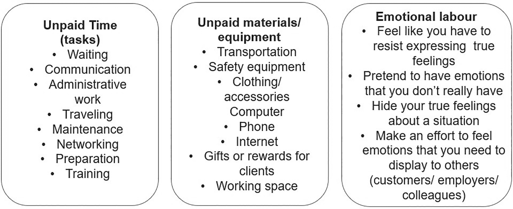
Figure 1. Different dimensions of unpaid labour.
Figure legend: The figure shows the different items that were used to measure unpaid labour time as tasks, unpaid material costs, and emotional labour.
3.1 Validating the measurement of the (unpaid) labour time dimension
To measure (unpaid) labour time, respondents were asked if a number of tasks (see Table 1) are part of their main job, and if so, to what extent they are paid. For the latent class analysis, these two variables have been recoded into one variable per task with three categories, indicating whether the task is 1=fully paid, no such work, 2= partially paid,
or 3 = fully unpaid.
Table 1. Survey-items used to measure (unpaid) labour time.
How frequently, if at all, do you do the following tasks as part of your main job? Daily/ Several times a week/Several times a month/Less often/Never
And in your main job, which, if any, of the following are paid for by your employer or client? Fully paid / Mostly paid, part of it not paid /Mostly not paid, part of it paid/Not paid at all
1. Waiting between tasks or clients
2. Communication with clients or employers (e.g., negotiating, email exchanges, meetings)
3. Administrative tasks or paperwork (e.g., dealing with HR, physical paperwork, writing reports)
4. Traveling between jobs and tasks (excluding commuting time between home and work)
5. Maintaining work equipment or tools
6. Networking (e.g., any efforts made to get more clients, orders, or business in the current job or maintain them over time, such as contacting or meeting people, attending events)
7. Preparing for the main task agreed by contract (e.g., getting ready or practicing or gathering materials for the main tasks, drawing up schedule or plan of the day)
8. Training for the main job (including workshops, conference)
Recoded to variables with 1=fully paid, no such work, 2= partially paid, 3 = fully unpaid
|
To construct the latent class model, we included all indicators on paid/unpaid tasks and compared model solutions with 1-6 latent classes.
Table 2 summarizes the information criteria used to compare the models. Based on these information criteria, we aimed to select the model with the fewest number of classes that best fits the data (Sinha et al., 2022). We see a strong decrease in the BIC and AIC (using an ‘elbow’ plot of fit) when looking at the models with 2 and with 3 classes, indicating an important increase in model fit. The BIC and AIC decrease further as the number of classes increases and are the lowest for the six-class solution, however the decrease is less substantial. The L-square statistic indicating the amount of the observed relationship between the variables that remains unexplained by a model has an acceptable p-value with 2 classes or more (the null hypothesis being that the model holds true in the population) (Magidson & Vermunt, 2004). Class entropy is the highest for the 2-class model (0,7184) and somewhat lower in the 3-class model (0,701), but still indicating an acceptable class separation (values of 0.6 or lower are generally not acceptable) for the 2 class and 3 class model (Weller et al., 2020). Next to information criteria, we also considered the number of sample members in each group, striving to avoid having classes containing less than 5% of the sample. We found that a solution of 4 or more classes always had at least one class with less than 5% of the sample members. Finally and importantly, we considered theoretical interpretability in choosing a solution (Weller et al., 2020). All these considerations led to selecting the 3 class solution. Although the BIC is not the lowest, the information criteria for model 3 are acceptable and it delivers the clearest interpretation of latent classes with each class having at least around 10% of class members, hence avoiding small ‘extreme’ classes. We considered models including the indicator on unpaid overtime, however, this did not deliver a clear solution; the scores of (unpaid) overtime appeared to follow a different pattern than those on (unpaid) tasks – indicating that respondents with high probabilities of unpaid overtime cannot be clustered together with those having a high probability of doing unpaid tasks.
Table 2. Comparison latent class models with indicators on unpaid tasks.
| LL | BIC (LL) | AIC (LL) | AIC3(LL) | Npar | L2 | df |
p-value
| Max. BVR | VLMR |
p-value
| Class.Err. | Entropy R2 |
|---|
| 1-Cluster | −35240,1 | 70627,37 | 70512,19 | 70528,19 | 16 | 23692,09 | 9869 | 5,0e-1128 | 1390,283 | | | 0 | 1 |
| 2-Cluster | −27828,1 | 55959,86 | 55722,3 | 55755,3 | 33 | 8868,201 | 9852 | 1 | 138,0233 | 14823,89 | 0 | 0,0524 | 0,7184 |
| 3-Cluster
| −26332,9
| 53125,73
| 52765,79
| 52815,79
| 50
| 5877,692
| 9835
| 1
| 34,9032
| 2990,509
| 0
| 0,0667
| 0,701
|
| 4-Cluster | −25854,3 | 52325,02 | 51842,7 | 51909,7 | 67 | 4920,601 | 9818 | 1 | 12,2886 | 957,0913 | 0 | 0,1347 | 0,6053 |
| 5-Cluster | −25608,4 | 51989,42 | 51384,73 | 51468,73 | 84 | 4428,628 | 9801 | 1 | 10,5558 | 491,9731 | 0 | 0,1428 | 0,596 |
| 6-Cluster | −25458,9 | 51846,8 | 51119,72 | 51220,72 | 101 | 4129,624 | 9784 | 1 | 9,6104 | 299,0041 | 0 | 0,1463 | 0,5962 |
The class profile of the three class solution can be found in Table 3. To interpret the classes in the selected three class solution, we look at the conditional item probabilities, that is the pattern of responses on the respective items per latent class (see Table 3). The first and largest class, containing 79% of the total sample, can be labelled as the ‘no unpaid tasks’ class: for each of the unpaid tasks, workers in this class have a very high probability (between 88,26% and 98,57%) of either not doing the task at all or being fully paid for it. The probability of doing the tasks and being only partially paid or not paid at all for it is very low for all tasks in this class, only training time has a somewhat higher, but still low, probability of being partially paid (6,52%) or fully unpaid (5,22%). The second class makes up 11.35% of the total sample and can be characterised as having a higher likelihood of spending time on tasks that are only partially paid than the other two classes – hence the label ‘partially unpaid tasks class’. While for some tasks in this class, such as waiting time and maintenance time, workers still have a higher probability of not doing the task or being fully paid for it, for all other tasks they are most likely to do the task while only being partially paid for it. We also detect a somewhat higher probability of doing fully unpaid tasks in class 2 than in class 1. The third class, which contains 9,65% of the sample, is labelled the ‘unpaid tasks’ class because workers have high probabilities (between 44,89% and 68, 28%) of doing the tasks fully unpaid. Especially communication time, administrative work, maintenance time, networking time, preparation time and training are very likely to be unpaid, for the other tasks the probability of being fully unpaid is somewhat lower but still significantly higher than in classes 1 and 2. This indicates the existence of an important group of workers (almost 10%) that does a number of tasks at work without receiving any payment for them.
Table 3. Class profile 3 class solution paid/unpaid tasks.
| | Class 1 ‘no unpaid tasks’ | Class 2 ‘partially unpaid tasks’ | Class 3 ‘unpaid tasks’ |
|---|
| Cluster size: % of sample | 79% | 11,35% | 9,65% |
| Waiting time
| Fully paid, no such work | 0,9857 | 0,6707 | 0,4716 |
| Partially paid | 0,0051 | 0,2621 | 0,0795 |
| Fully unpaid | 0,0092 | 0,0672 | 0,4489 |
| Communication time
| Fully paid, no such work | 0,9748 | 0,4676 | 0,1812 |
| Partially paid | 0,009 | 0,4975 | 0,136 |
| Fully unpaid | 0,0162 | 0,0349 | 0,6828 |
| Administrative work
| Fully paid, no such work | 0,9829 | 0,3938 | 0,2153 |
| Partially paid | 0,0115 | 0,57 | 0,1279 |
| Fully unpaid | 0,0056 | 0,0362 | 0,6568 |
| Training time
| Fully paid, no such work | 0,8826 | 0,3747 | 0,3397 |
| Partially paid | 0,0652 | 0,4915 | 0,1707 |
| Fully unpaid | 0,0522 | 0,1338 | 0,4896 |
| Maintenance time
| Fully paid, no such work | 0,9756 | 0,5776 | 0,375 |
| Partially paid | 0,0112 | 0,3606 | 0,045 |
| Fully unpaid | 0,0132 | 0,0618 | 0,58 |
| Networking time
| Fully paid, no such work | 0,9296 | 0,309 | 0,3038 |
| Partially paid | 0,0535 | 0,5706 | 0,0504 |
| Fully unpaid | 0,0169 | 0,1205 | 0,6457 |
| Preparation time
| Fully paid, no such work | 0,9701 | 0,3065 | 0,2432 |
| Partially paid | 0,0211 | 0,6592 | 0,1659 |
| Fully unpaid | 0,0088 | 0,0343 | 0,591 |
| Training
| Fully paid, no such work | 0,9078 | 0,3381 | 0,3446 |
| Partially paid | 0,0778 | 0,596 | 0,1094 |
| Fully unpaid | 0,0144 | 0,0659 | 0,546 |
The following step in the analysis added country as a covariate to the model, aiming to test whether the classes are the same across countries. After determining the required number of classes for each group (in our case three classes in each country), we compared different degrees of measurement equivalence, aiming to select “the model with the lowest level of inequivalence possible that fits the data well” (Kankaraš et al., 2018, p.369). This is done by first fitting the model with the least amount of measurement equivalence to the data, followed by a series of nested, restricted models that are evaluated in terms of model fit.
Table 4 contains the model statistics for each model. The heterogeneity model has the least amount of measurement equivalence because all parameters are allowed to differ across groups. In fact, it is equal to estimating a latent class model in each country separately. Concluding that a measurement model is heterogeneous means that both the connection to the latent classes and the baselines (or ‘intercepts’) of the different classes differ across the countries. The partial homogeneity model is estimated by constraining the interaction terms to zero - meaning that the relationships between the latent classes (in our case the “no unpaid tasks”, “partially paid tasks” and “unpaid tasks” classes) and the indicators (such as waiting time, administrative work etc.) do not differ by group. However, the partial homogeneity model still allows direct effects of the group variable on the indicators – meaning the baselines of unpaid labour differs across countries. The structural homogeneity model has an even higher level of measurement equivalence, as both the interactions and the direct effects between the grouping variable and the indicators are constrained to zero. As a result, conditional probabilities of items are restricted to be equal across the groups and independent from the grouping variable, when controlled for the latent variable. The only aspect left to vary is the probability of class membership. The complete homogeneity model, which represents the highest level of equivalence, is equal to a single-group latent class model and asserts that latent classes are identical across all groups (Lukac et al., 20191). As Table 4 shows, model fit is the highest in the structural homogeneity model - as indicated by the lowest value of the BIC statistic (AIC and AIC3 are even lower in the heterogenous model but BIC is the more telling statistic (Nylund-Gibson & Choi, 2018). This indicates a high level of measurement equivalence facilitating comparison of our classes across countries, while still allowing the size of the classes to vary across countries. Hence, we select the structural homogeneity model with three classes based on which we obtain the classifications of individuals to the class they most likely belong to, using their posterior class membership probabilities. We obtain three new variables in the dataset, which can be used to examine the relationship between class membership and other variables of interest.
Table 4. Comparison model fit with different degrees of measurement (in)equivalence.
|
LL |
BIC (LL) |
AIC (LL) |
AIC3(LL) | Npar | Max. BVR | Class.Err. | Entropy R2 |
|---|
| heterogeneity
| −25913,7 | 53667,19 | 52227,435 | 52427,435 | 200 | 34,9869 | 0,0708 | 0,7639 |
| partial homogeneity
| −26085 | 53126,627 | 52377,955 | 52481,955 | 104 | 33,5311 | 0,0714 | 0,6928 |
| structural homogeneity
| −26281,7 | 53078,525 | 52675,393 | 52731,393 | 56 | 36,9317 | 0,0715 | 0,6958 |
| complete homogeneity
| −26332,9 | 53125,728 | 52765,79 | 52815,79 | 50 | 34,9032 | 0,0667 | 0,701 |
3.2 Validating the measurement of the (unpaid) material resources dimension
To measure (unpaid) material resources, respondents were asked if they needed certain tools/equipment for their main job, and if so, to what extend buying or maintaining these were paid (cf. Table 5). For the latent class analysis, these two variables were recoded to one variable with categories 1=Fully paid or not needed and 2=Partially or fully unpaid. Moreover, we measured whether workers own the tools and equipment they need for their work and whether the expenses for using them are covered by themselves or by the company (cf. Table 5). This was recoded into two variables, one for ownership with categories 1 = I own it and 2 = My company owns it and one variable for covering expenses for use, with 1= I cover the expenses for use, and 2= My company covers the expenses for use.
Table 5. Survey-items used to measure (unpaid) material resources.
Do you need the following for your main job? Original categories: Yes/No
Are the expenses for buying or maintaining the following paid for by your employer or client? Original categories: Fully paid / Mostly paid, part of it not paid /Mostly not paid, part of it paid/Not paid at all
Transportation used during working hours (e.g., car, bike, truck, etc.), excluding commuting between home and work
Safety equipment (e.g., personal protective equipment or PPE, gloves, etc.)
Specific clothing or accessories (including uniform)
Computer (e.g., PC, laptop, tablet, and other connected device)
Phone
Internet
Gifts or rewards for clients (including business dinners)
Working space
Recoded to one variable on expenses for buying or maintaining materials with categories:
Who owns the following and who covers the expenses for using it?
Original categories: I own it and I cover its expenses/I own it but my company covers its expenses/ My company owns it but I cover its expenses/My company owns and covers its expenses
Transportation used during working hours (e.g., car, bike, truck, etc.), excluding commuting between home and work
Safety equipment (e.g., personal protective equipment or PPE, gloves, etc.)
Specific clothing or accessories (including uniform)
Computer (e.g., PC, laptop, tablet, and other connected device)
Phone
Internet
Recoded to one variable on ownership of materials, categories:
1.
I own it
2.
My company owns it
|
3.2.1 Latent class analysis on expenses for buying or maintaining materials
As the number of valid cases in the ‘partially or fully unpaid’ category is very low for gifts (1,9%), safety equipment (4%) and specific clothing or accessories (7,3%), these items were left out from the latent class analysis, but remain in the dataset and may be used for other analyses. All other indicators on expenses for buying or maintaining materials were included in the model.
Table 6 summarizes the information criteria used to compare model solutions with 1-6 latent classes. We see a strong decrease in the BIC (using an ‘elbow’ plot of fit) when looking at the models with 2 and with 3 classes, indicating an important increase in model fit. The BIC decreases further as the number of classes increases and are the lowest for the four-class solution, however the decrease is less substantial. The L-square statistic indicating the amount of the observed relationship between the variables that remains unexplained by a model becomes unsignificant with 4 classes or more. Class entropy is the highest for the 2-class model (0,6506) and slightly lower in the 3-class model (0,6446), but still indicating an acceptable class separation. We also considered the number of sample members in each group and found that a solution of 4 or more classes always had at least two ‘smaller’ classes containing 10% or less than of the sample members. Finally and importantly, we considered theoretical interpretability in choosing a solution. We selected the 3 class solution, which is the model with the fewest number of classes and an acceptable fit with the data that delivers a clear theoretical interpretation.
Table 6. Comparison latent class models with indicators on expenses for buying and maintaining work equipment.
| LL | BIC (LL) | AIC (LL) | AIC3(LL) | Npar | L2 | df |
p-value
| Max. BVR | VLMR |
p-value
| Class.Err. | Entropy R2 |
|---|
| 1-Cluster | −18640,7 | 37327,48 | 37291,49 | 37296,49 | 5 | 6836,47 | 179 | 9,8e-1308 | 2807,479 | | | 0 | 1 |
| 2-Cluster | −15684,8 | 31470,71 | 31391,52 | 31402,52 | 11 | 924,5055 | 173 | 5,8E-103 | 260,0334 | 5911,965 | 0 | 0,0847 | 0,6506 |
| 3-Cluster | −15361,9 | 30880,12 | 30757,74 | 30774,74 | 17 | 278,7211 | 167 | 1,30E-07 | 16,1055 | 645,7845 | 0 | 0,102 | 0,6446 |
| 4-Cluster | −15299,9 | 30811,33 | 30645,76 | 30668,76 | 23 | 154,7405 | 161 | 0,62 | 4,0125 | 123,9806 | 0 | 0,1615 | 0,5521 |
| 5-Cluster | −15285,1 | 30837 | 30628,23 | 30657,23 | 29 | 125,2188 | 155 | 0,96 | 0,0411 | 29,5217 | 0 | 0,1493 | 0,5787 |
| 6-Cluster | −15284,3 | 30890,53 | 30638,58 | 30673,58 | 35 | 123,5621 | 149 | 0,94 | 0,0105 | 1,6566 | 0,6045 | 0,1897 | 0,5223 |
The class profile of the three class solution can be found in Table 7. To interpret the classes in the selected three class solution, we look at the conditional item probabilities, that is the pattern of responses on the respective items per latent class (see Table 7). The first and largest class, containing 67,11% of the total sample, can be labelled as the ‘no unpaid expenses’ class: for each of the items, workers in this class have a very high probability (between 87,98% and 99,98%) of not needing them or being fully paid for buying and maintaining them. The probability of needing the items but not having the expenses covered by a client or employer is very low for all items in this class. The second class makes up 25.13% of the total sample and can be characterised as having a high likelihood of not needing or being fully paid for transportation, computers and phones, but often facing internet- (conditional item probability of 79,81%) and sometimes workspace-related (50,21%) expenses - hence the label ‘unpaid internet and workspace expenses’. This finding is interesting as it indicates the existence of an important group of workers (around ¼ of the population) that needs the internet for their work but often does not see the costs of internet use covered. The third and smallest class, which contains 7,76% of the sample, is labelled the ‘unpaid material expenses’ class because workers are likely to face expenses uncompensated by clients or employers. Especially expenses for buying and maintaining computers, phones and internet are very likely to be unpaid (between 95,35% and 98,97%), these probabilities are somewhat lower for workspace- and (68,36%) and transportation-related (53,14%) costs. This indicates the existence of an group of workers (almost 8%) that does not receive (full) payment for the equipment needed to execute their work.
Table 7. Class profile 3 class solution expenses for buying and maintaining work equipment.
| |
Class 1 ‘no unpaid expenses’ |
Class 2 ‘unpaid internet and workspace expenses’ |
Class 3 ‘unpaid material expenses’ |
|---|
| Cluster Size
| 67,11%
| 25,13%
| 7,76%
|
| Transp_d
| Fully paid, not needed | 0,8798 | 0,7743 | 0,4686 |
| Partially or fully unpaid | 0,1202 | 0,2257 | 0,5314 |
| PC_d
| Fully paid, not needed | 0,9905 | 0,897 | 0,034 |
| Partially or fully unpaid | 0,0095 | 0,103 | 0,966 |
| Phone_d
| Fully paid, not needed | 0,9194 | 0,6899 | 0,0103 |
| Partially or fully unpaid | 0,0806 | 0,3101 | 0,9897 |
| Internet_d
| Fully paid, not needed | 0,9998 | 0,2019 | 0,0465 |
| Partially or fully unpaid | 0,0002 | 0,7981 | 0,9535 |
| Workspace_d
| Fully paid, not needed | 0,9938 | 0,4979 | 0,3164 |
| Partially or fully unpaid | 0,0062 | 0,5021 | 0,6836 |
The following step in the analysis added country as a covariate to the model, aiming to test whether the classes are the same across countries.
Table 8 compares the model statistics for models with different degrees of measurement equivalence. As Table 4 shows, model fit is the highest in the partial homogeneity model - as indicated by the lowest value of the BIC, AIC and AIC3 statistics. This indicates a relatively high level of measurement equivalence facilitating comparison of our classes across countries, as the relationships between the latent classes and the indicators does not differ between countries. However, the size of the three classes and the baseline of unpaid expenses (direct effects) are still allowed to vary across countries. Hence, case classifications are obtained using the posterior class membership probabilities of the partial homogeneity model.
Table 8. Comparison model fit with different degrees of measurement (in)equivalence.
| LL | BIC (LL) | AIC (LL) | AIC3(LL) | Npar | L2 | df | p-value
| Max. BVR | Class.Err. | Entropy R2 |
|---|
| heterogeneity
| −15052,6 | 30730,73 | 30241,22 | 30309,22 | 68 | 330,7648 | 305 | 0,15 | 15,2542 | 0,1113 | 0,6316 |
| partial homogeneity
| −15072,2 | 30494,02 | 30220,46 | 30258,46 | 38 | 370,012 | 335 | 0,091 | 16,3073 | 0,1089 | 0,6366 |
| structural homogeneity
| −15166,6 | 30544,81 | 30379,24 | 30402,24 | 23 | 558,7843 | 350 | 8,20E-12 | 16,44 | 0,1082 | 0,6477 |
| complete homogeneity
| −15361,9 | 30880,12 | 30757,74 | 30774,74 | 17 | 278,7211 | 167 | 1,30E-07 | 16,1055 | 0,102 | 0,6446 |
3.2.2 Latent class analysis on ownership of materials
We included all indicators on ownership of work materials/equipment in the model and compared model solutions with 1-6 latent classes.
Table 9 shows a strong decrease in the BIC and AIC (using an ‘elbow’ plot of fit) when looking at the model with 2 classes, indicating an important increase in model fit. The BIC and AIC decrease further as the number of classes increases and are the lowest for the four (BIC) and (AIC) class solution, however the decrease is less substantial. Class entropy is acceptable for the 2-class model (0,5983) and substantially lower in the other models. Solutions up to four classes had more than 10% in each cluster, but these smaller classes were harder to interpret theoretically. We selected the 2 class solution because it delivered the most clear theoretical interpretation, with each class including a significant share of the workforce.
Table 9. Comparison latent class models with indicators on ownership of work equipment.
| LL | BIC (LL) | AIC (LL) | AIC3(LL) | Npar | L2 | df |
p-value
| Max. BVR | VLMR | p-value
| Class.Err. | Entropy R2 |
|---|
| 1-Cluster | −15263,4 | 30582,02 | 30538,83 | 30544,83 | 6 | 7878,699 | 659 | 4,2e-1216 | 1999,956 | | | 0 | 1 |
| 2-Cluster | −12543,8 | 25207,25 | 25113,67 | 25126,67 | 13 | 2439,538 | 652 | 3,7E-204 | 212,9975 | 5439,161 | 0 | 0,0781 | 0,5983 |
| 3-Cluster | −12352 | 24888,05 | 24744,07 | 24764,07 | 20 | 2055,938 | 645 | 9,7E-147 | 91,9566 | 383,5999 | 0 | 0,2748 | 0,4296 |
| 4-Cluster | −12226,5 | 24701,43 | 24507,06 | 24534,06 | 27 | 1804,93 | 638 | 5,8E-112 | 3,0522 | 251,0075 | 0 | 0,3079 | 0,4011 |
| 5-Cluster | −12207,7 | 24728,08 | 24483,32 | 24517,32 | 34 | 1767,185 | 631 | 3E-108 | 2,9249 | 37,7456 | 0 | 0,4168 | 0,3532 |
| 6-Cluster | −12199,4 | 24775,91 | 24480,76 | 24521,76 | 41 | 1750,625 | 624 | 1,7E-107 | 2,416 | 16,56 | 0,0046 | 0,3892 | 0,3603 |
The class profile of the 2-class solution can be found in Table 10. Looking at the conditional item probabilities, the first and largest class, containing 80,96% of the total sample, can be labelled as the ‘company-owned class: there is a very high probability (between 81,24% and 99,26%) that the tool is owned by the company, only for transportation this probability is somewhat lower (58,75%). The second class, containing 19,04% of the sample, is labelled the ‘self-owned’ class because workers have high probabilities (between 69,75% and 97, 16%) of owning this equipment. The resulting class membership can be used to distinguish between those workers owning the materials they need for work and those workers who don’t own them.
Table 10. Class profile 2 class solution ownership of work equipment.
| | Class 1 ‘company-owned’ | Class 2 ‘self-owned’ |
|---|
| Cluster Size
| 80,96% | 19,04% |
|
Transp_Ownership_d
| I own it | 0,4125 | 0,8946 |
| My company owns it | 0,5875 | 0,1054 |
|
Safety_Ownership_d
| I own it | 0,0901 | 0,791 |
| My company owns it | 0,9099 | 0,209 |
|
Appearance_Ownership_d
| I own it | 0,1876 | 0,8604 |
| My company owns it | 0,8124 | 0,1396 |
|
PC_Ownership_d
| I own it | 0,0074 | 0,6975 |
| My company owns it | 0,9926 | 0,3025 |
|
Phone_Ownership_d
| I own it | 0,131 | 0,9716 |
| My company owns it | 0,869 | 0,0284 |
|
Internet_Ownership_d
| I own it | 0,1481 | 0,9067 |
| My company owns it | 0,8519 | 0,0933 |
The following step compared different degrees of measurement equivalence, first fitting the model with the least amount of measurement equivalence to the data, followed by a series of restricted models that are evaluated in terms of model fit. As Table 11 shows, model fit is the highest in the partial homogeneity model - as indicated by the lowest value of the BIC statistic (AIC and AIC3 are slightly lower in the heterogenous model but BIC is the more telling statistic). Classes can be compared, while still allowing the size of the classes and the baselines of the indicators to vary across countries. Hence, we select the partial homogeneity model with three classes based on which we obtain the classifications of individuals to the class they most likely belong to. This creates two variables in the dataset based on which the relationship of class membership with other variables can be analysed while taking into account the effect of country on latent class indicators.
Table 11. Comparison model fit with different degrees of measurement (in)equivalence.
| LL | BIC (LL) | AIC (LL) | AIC3(LL) | Npar | L2 | df | p-value
| Max. BVR | Class.Err. | Entropy R2 |
|---|
| heterogeneity
| −12048,1 | 24574,55 | 24200,22 | 24252,22 | 52 | 3551,276 | 2508 | 2,00E-39 | 212,3053 | 0,0816 | 0,5971 |
| partial homogeneity
| −12081 | 24474,69 | 24229,93 | 24263,93 | 34 | 3616,994 | 2526 | 2,70E-42 | 218,7576 | 0,0812 | 0,5951 |
| structural homogeneity
| −12348,8 | 24844,78 | 24729,6 | 24745,6 | 16 | 4152,662 | 2544 | 4,20E-81 | 205,1102 | 0,0966 | 0,5857 |
| complete homogeneity
| −12543,8 | 25207,25 | 25113,67 | 25126,67 | 13 | 2439,538 | 652 | 3,7E-204 | 212,9975 | 0,0781 | 0,5983 |
3.2.3 Latent class analysis on expenses for use of materials
We compared model solutions with 1-6 latent classes containing all indicators on expenses for use of materials.
Table 12 summarizes the information criteria used to compare the models. Based on these information criteria, we aimed to select the model with the fewest number of classes that best fits the data (Sinha et al., 2022). We see a strong decrease in the BIC and AIC (using an ‘elbow’ plot of fit) when looking at the models with classes, indicating an important increase in model fit. The BIC and AIC decrease further as the number of classes increases and are the lowest for the four-class solution, however the decrease is much smaller. Class entropy is the highest for the 2-class model (0,602) and lower than the acceptable value of 0,6 for all other models. Looking at the number of sample members in each group, we found that a solution of 4 or more classes always had at least two classes containing less than 10% of the sample members. Finally and importantly, we considered theoretical interpretability in choosing a solution (Weller et al., 2020). All these considerations led to selecting the 2 class solution.
Table 12. Comparison latent class models with indicators on expenses for use of work equipment.
| LL | BIC (LL) | AIC (LL) | AIC3(LL) | Npar | L2 | df |
p-value
| Max. BVR | VLMR |
p-value
| Class.Err. | Entropy R2 |
|---|
| 1-Cluster | −14074,2 | 28203,68 | 28160,49 | 28166,49 | 6 | 7342,21 | 659 | 1,2e-1109 | 1895,679 | | | 0 | 1 |
| 2-Cluster | −11355,3 | 22830,27 | 22736,69 | 22749,69 | 13 | 1904,41 | 652 | 7,2E-123 | 57,7588 | 5437,801 | 0 | 0,0706 | 0,6027 |
| 3-Cluster | −11234,3 | 22652,65 | 22508,67 | 22528,67 | 20 | 1662,396 | 645 | 6,70E-91 | 34,666 | 242,0138 | 0 | 0,2102 | 0,4236 |
| 4-Cluster | −11190,6 | 22629,55 | 22435,19 | 22462,19 | 27 | 1574,911 | 638 | 8,30E-81 | 3,542 | 87,4848 | 0 | 0,2033 | 0,4068 |
| 5-Cluster | −11183 | 22678,69 | 22433,93 | 22467,93 | 34 | 1559,653 | 631 | 3,30E-80 | 3,0734 | 15,2577 | 0,0265 | 0,3313 | 0,3236 |
| 6-Cluster | −11180,2 | 22737,5 | 22442,35 | 22483,35 | 41 | 1554,069 | 624 | 7,20E-81 | 3,4097 | 5,5843 | 0,1891 | 0,39 | 0,3139 |
The class profile of the two-class solution can be found in Table 13. The first and largest class, containing 82,69% of the total sample, is labelled the ‘company-covered expenses’ class: for every equipment, the probability that the company covers the expenses for use is between 75,3% and 98,88%. The probability that workers cover the expenses themselves is lower than 15%, except for transportation costs (24,7%). The second class makes up 17,31% of the total sample and can be characterised as having a higher likelihood of workers covering the expenses for use of equipment themselves. Conditional item probabilities vary between 67,64% and 93,74%, which especially transportation, phone and internet expenses likely to be paid by workers themselves. This indicates the existence of an important group of workers that has to manage these expenses without receiving compensation for them.
Table 13. Class profile 2 class solution expenses for use of work equipment.
| | Class 1 ‘company-covered expenses’ | Class 2 ‘self-covered expenses’ |
|---|
| Cluster Size
| 82,69% | 17,31% |
| Transp_Expenses
| I cover the expenses for use
| 0,247 | 0,8195 |
| My company covers the expenses for use
| 0,753 | 0,1805 |
| Safety_Expenses
| I cover the expenses for use
| 0,0212 | 0,6764 |
| My company covers the expenses for use
| 0,9788 | 0,3236 |
| Appearance_Expenses
| I cover the expenses for use
| 0,1051 | 0,7805 |
| My company covers the expenses for use
| 0,8949 | 0,2195 |
| PC_Expenses
| I cover the expenses for use
| 0,0112 | 0,7129 |
| My company covers the expenses for use
| 0,9888 | 0,2871 |
| Phone_Expenses
| I cover the expenses for use
| 0,1122 | 0,9374 |
| My company covers the expenses for use
| 0,8878 | 0,0626 |
| Internet_Expenses
| I cover the expenses for use
| 0,1407 | 0,9284 |
| My company covers the expenses for use
| 0,8593 | 0,0716 |
Looking at measurement equivalence across countries, Table 14 shows, the lowest value of the BIC statistic in the partial homogeneity model. We select this model to obtain classifications, indicating that the latent classes can be compared across countries, when allowing the size of the classes and the baselines of the indicators to vary.
Table 14. Comparison model fit with different degrees of measurement (in)equivalence.
| LL | BIC (LL) | AIC (LL) | AIC3(LL) | Npar | L2 | df | p-value
| Max. BVR | Class.Err. | Entropy R2 |
|---|
| heterogeneity
| −10901,1 | 22280,52 | 21906,18 | 21958,18 | 52 | 3040,336 | 2508 | 8,90E-13 | 54,7559 | 0,0793 | 0,5908 |
| partial homogeneity
| −10929,9 | 22172,61 | 21927,85 | 21961,85 | 34 | 3098,002 | 2526 | 2,80E-14 | 55,4602 | 0,0754 | 0,5964 |
| structural homogeneity
| −11150,9 | 22449,08 | 22333,9 | 22349,9 | 16 | 3540,051 | 2544 | 4,80E-36 | 60,311 | 0,0905 | 0,5886 |
| complete homogeneity
| −11355,3 | 22830,27 | 22736,69 | 22749,69 | 13 | 1904,41 | 652 | 7,2E-123 | 57,7588 | 0,0706 | 0,6027 |
3.3 Validating the measurement of the emotional effort dimension
To measure emotional effort, respondents were asked how often they had to make the emotional efforts listed in Table 15. For the latent class analysis, the items were recoded to binary items with category 1=effort is part of job and category 2=effort is not (or only rarely) part of job. The items do not specify whether the efforts are paid for.
Table 15. Survey-items used to measure (unpaid) emotional effort.
In your main job, how often, if at all, do you … ?
Feel like you have to resist expressing your true feelings
Pretend to have emotions that you don’t really have
Hide your true feelings about a situation
Make an effort to feel emotions you need to display to others (customers, employers, or colleagues)
Original answer categories: Never/Rarely/Sometimes/Most of the time/Always
Recoded answer categories:
1= Rarely/Never: ‘emotional effort is not (or only rarely) part of the job’
2= Always/Most of the time/Sometimes: ‘emotional effort is part of the job’
|
We included all recoded indicators on emotional labour in the model and compared model solutions with 1-6 latent classes.
Table 16 summarizes the information criteria used to compare the models. Based on these information criteria, we aimed to select the model with the fewest number of classes that best fits the data. We see the strongest decrease in the BIC and AIC (using an ‘elbow’ plot of fit) when looking at the models with 2 classes, indicating an important increase in model fit. The BIC and AIC decrease further with the three-class solution where they are the lowest, however, this decrease is much less substantial. The L-square statistic indicating the amount of the observed relationship between the variables that remains unexplained by a model has an acceptable p-value with three classes or more (the null hypothesis being that the model holds true in the population). Class entropy is the highest for the 2-class model (0,6109) and decreases to values lower than the acceptable class separation value of 0,6 in the 3-class model (0,5421) and the following models. Regarding sample size in each group, all 1-6 class solutions have classes containing more than 5% of the sample, although solutions with 4-6 classes always contain multiple classes no more than 15% of the sample. Finally and importantly, we considered theoretical interpretability in choosing a solution. All these considerations led to selecting the 2-class solution. It delivers the clearest interpretation and seperation of latent classes with conditional item probabilities of 0,72 or higher. Each of the two classes contains a substantial share of class members, hence avoiding small ‘extreme’ classes.
Table 16. Comparison latent class models with indicators on emotional labour.
| | LL | BIC (LL) | AIC (LL) | AIC3(LL) |
Npar |
L2 | df |
p-value
| Max. BVR |
VLMR |
p-value
| Class.Err. | Entropy R2 |
|---|
| Model1
| 1-Cluster | −21071,5 | 42179,843 | 42151,048 | 42155,048 | 4 | 7011,835 | 42 | 8,2e-1471 | 2418,17 | | | 0 | 1 |
| Model2
| 2-Cluster | −17750,7 | 35584,212 | 35519,423 | 35528,423 | 9 | 370,21 | 37 | 1,40E-56 | 79,9661 | 6641,625 | 0 | 0,1541 | 0,6109 |
| Model3
| 3-Cluster | −17583,3 | 35295,295 | 35194,512 | 35208,512 | 14 | 35,299 | 32 | 0,31 | 0,5719 | 334,911 | 0 | 0,2276 | 0,5421 |
| Model4
| 4-Cluster | −17579,6 | 35333,934 | 35197,157 | 35216,157 | 19 | 27,9445 | 27 | 0,41 | 0,0004 | 7,3545 | 0,0277 | 0,3265 | 0,4452 |
| Model5
| 5-Cluster | −17579,6 | 35379,926 | 35207,156 | 35231,156 | 24 | 27,943 | 22 | 0,18 | 0,0004 | 0,0015 | 0,2654 | 0,3737 | 0,3934 |
| Model6
| 6-Cluster | −17579,6 | 35425,92 | 35217,155 | 35246,155 | 29 | 27,9426 | 17 | 0,046 | 0,0004 | 0,0004 | 0,7472 | 0,3827 | 0,3635 |
The class profile of the 2-class solution can be found in Table 17. To interpret the classes, we look at the conditional item probabilities, that is the pattern of responses on the respective items per latent class (see Table 17). Both classes make up around half of the total sample. The first class can be characterised as having a low likelihood of spending emotional efforts – hence the label ‘no (or very little) emotional labour’ class. While we detect a somewhat higher probability (around 28%) of making an effort to feel emotions you need to display to others (customers, employers, or colleagues), for all other kinds of emotional labour the probability of constant, frequent or some exposure is no higher than a forth (24%). The second class can be labelled as the ‘emotional labour’ class: for each kind of emotional labour measured, workers in this class have a high probability (between 67% and 95%) of always, often or sometimes doing this kind of labour. The probability of never or only rarely making these efforts is very low in this class, only pretending to have emotions that you don’t really have has a somewhat higher probability (33%). These findings indicate the widespread existence of emotional labour in half of the working population, while the other half of the working population appears to be more shielded from these efforts.
Table 17. Class profile 2 class solution paid/unpaid tasks.
| | Class 1 ‘no (or very little) emotional labour’ | Class 2 ‘emotional labour’ |
|---|
| Cluster Size
| 49,97% | 50,03% |
| Surpress Feelings
| effort is not part of job | 0,7559 | 0,0833 |
| effort is part of job | 0,2441 | 0,9167 |
| Pretend Emotions
| effort is not part of job | 0,9665 | 0,3313 |
| effort is part of job | 0,0335 | 0,6687 |
| Hide Feelings
| effort is not part of job | 0,8165 | 0,0533 |
| effort is part of job | 0,1835 | 0,9467 |
| Effort Emotions
| effort is not part of job | 0,7146 | 0,2648 |
| effort is part of job | 0,2854 | 0,7352 |
Table 18 shows that the heterogeneity model has the best model fit. That means researchers need to take into account measurement inequivalence and allow both the connection of indicators to the latent classes and the baselines (or ‘intercepts’) of the different classes differ across countries. Based on this model, classifications of individuals to the class they most likely belong to were obtained by using their posterior class membership probabilities. These classifications result in new variables in the dataset that account for interdependence between the country variable and latent class indicators.
Table 18. Comparison model fit with different degrees of measurement (in)equivalence.
| LL | BIC (LL) | AIC (LL) | AIC3(LL) | Npar | L2 | df | p-value
| Max. BVR | Class.Err. | Entropy R2 |
|---|
| heterogenity
| −17058,8 | 34448,79 | 34189,64 | 34225,64 | 36 | 451,2575 | 76 | 1,10E-54 | 33,1853 | 0,1369 | 0,6193 |
| partial homogenity
| −17186,1 | 34592,94 | 34420,17 | 34444,17 | 24 | 705,7858 | 88 | 3,70E-97 | 62,8169 | 0,1488 | 0,6104 |
| structural homogenity
| −17608,7 | 35327,77 | 35241,39 | 35253,39 | 12 | 1551,007 | 100 | 1,1E-258 | 110,1414 | 0,138 | 0,6172 |
| complete homogenity
| −17750,7 | 35584,21 | 35519,42 | 35528,42 | 9 | 370,21 | 37 | 1,40E-56 | 79,9661 | 0,1541 | 0,6109 |
Ethics and consent
Prior to starting the research, the project received approval by the ethical committee SMEC (Sociaal-maatschappelijke Ethische Commissie) – file number G-2019 07 1689, register numbers G-2019-1344-R6 and G-2023-6972.
Written informed consent was obtained from the participants of the national survey panels (see B.2 Ethical considerations for details).









