1. Introduction
Climate change is expected to have significant impacts on human wellbeing and ecosystems, particularly by altering the hydrologic cycle and reducing water availability (Gøtske and Victoria, 2021; Granados et al., 2021). At the same time, water demand is projected to increase due to population and economic growth, rising temperatures, and changing precipitation patterns. Currently, approximately 52 million people (11% of the population) in the 27 European Union (EU) member states and the United Kingdom live in water-scarce regions, and this situation is likely to worsen with climate change (Bisselink et al., 2020). Managing water supplies effectively during periods of low availability is crucial to meet demand and avoid competition among users, especially under future climate conditions (De Roo et al., 2023).
Climate change may imply changes in both annual water availability and required storage capacity. The way these two changes combine can inform decision-makers about the need to adjust water demand, develop additional water storage or a combination of the two (Đorđević and Dašić, 2011; World Bank, 2023). Reducing water demand is often considered a no-regret option, as it can help control costs and alleviate pressure on water ecosystems, even in the absence of climate change. Increasing storage capacity attenuates the reduction of water availability and reduces its uncertainty under climate change projections (Granados et al., 2021).
Water demand reduction can be achieved by improving water system efficiency, such as controlling leakages, implementing real-time control, and enhancing forecasting and operation (e.g., reservoir management). Alternative water resources, including water reuse (Pistocchi et al., 2018), rainwater and atmospheric water harvesting, and desalination (Pistocchi et al., 2020), can also be mobilized.
Water storage capacity can be increased by building single- or multi-purpose reservoirs with various sizes and design options (Jurik et al., 2015; Mioduszewski, 2012, Watts et al., 2011; Schmitt and Rosa, 2024; Bahri, 2020), managed aquifer recharge (Sprenger et al., 2017), and improved water management at the landscape scale, e.g. by preserving soil water holding capacity (García-Tejero et al., 2019) and retention in wetlands.
Quantifying demand reduction and storage needs is essential for developing effective adaptation strategies in integrated water resources management (IWRM; GWP and INBO, 2009). Planning, design and optimization methods for water resources are well established for watershed- and local scale applications (e.g. Loucks and van Beek, 2017), usually entailing complex methods and specific data. Here we propose a novel and efficient method for a screening-level quantification of adaptation needs by identifying storage capacity gaps (World Bank, 2023) together with availability trends at a regional scale, based on the processing of results from hydrological simulation models increasingly available at the global level. In this way, we can support decisions at the strategic planning level (e.g. identification of the order of magnitude of investments and the required funds), before delving into more complex assessments in specific river basins (e.g., Al-Jawad et al., 2019). With our approach, daily streamflow time series from a regional spatially distributed hydrological model are used to quantify annual water availability and storage capacity requirements to satisfy a given water demand pattern by buffering the intra-annual variability of available water.
After describing the method in detail, we demonstrate its application to estimate the order of magnitude of additional water storage volumes required because of climate change in Europe.
2. Materials and methods
We consider an ensemble of daily river flow time series simulated through a complex spatially distributed hydrological model for Europe under climate change scenarios. For each time series we calculate two indicators, the first defined here as the “storage rate” or fraction of the annual water demand volume that needs to be stored to buffer water availability. The other is simply the total water volume available each year to meet a given demand. The two indicators are calculated for every year. The combination of the trends in the two resulting yearly time series allows to classify a river basin in terms of the type of adaptation action it may require, whether on demand reduction, on storage capacity increase, or a combination of both.
The storage rate
The well-known “mass curve analysis” (Rippl, 1883) is a quick way to estimate the reservoir volume required to buffer a time-varying water inflow
and matches a prescribed outflow
, with reference to a period during which the sum of inflows equals the sum of outflows. One way to implement this analysis is to calculate the running sum of inflows (i.e., availability) and outflows (i.e., demand) over a reference period and calculate the amplitude of the maximum positive and negative (absolute value) deviation between the two. The sum of the two deviations represents the required volume V, i.e.:
[Eq. 1]
The mass curve analysis is a practical engineering approach to the sizing of reservoirs. Here we show how it can be used in a more general way to quantify the storage capacity required to meet a water demand with a given distribution in time, using water available with a different time distribution. To this end, we have to assume that demand is equal to availability, i.e. we focus on the share of demand that can be actually met by the available water. When demand equals availability over a year, we do not need to quantify the total yearly volume of demand, but only its relative distribution in time. Therefore we consider a demand pattern, i.e. a normalized demand distribution for which the yearly sum is identically equal to 1. Consistently, an appropriate normalized distribution of availability is obtained by dividing the available streamflow at every step by the sum of values at all time steps in the year, so that the yearly sum equals 1 for every year. We then apply Eq. 1 with reference to a given year, using for
the streamflow in a catchment divided by the annual total, as a proxy of water availability, and for
a demand compatible with availability (i.e. whose annual volume is equal to the annual volume available) and following a predefined temporal pattern.
As we use normalized quantities, the required storage volume is calculated dimensionless as a storage volume per unit of demand volume, hence we call it the “storage rate”.
Figure 1 illustrates this concept.
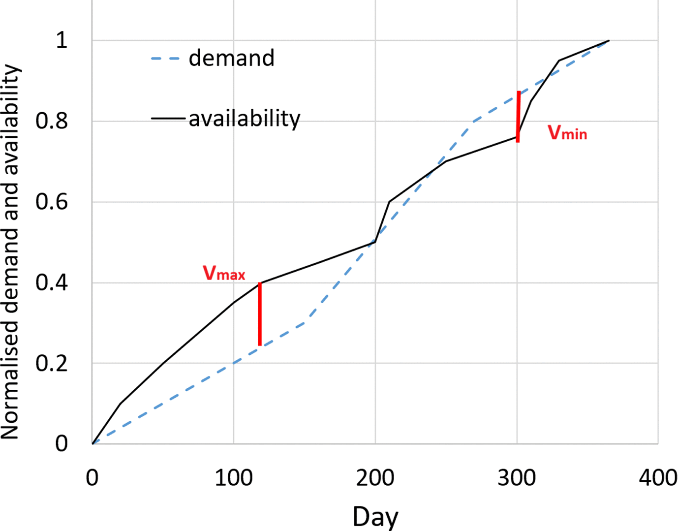
Figure 1. Calculation of the storage rate.
The fraction of the annual demand volume to be stored is Vmax+|Vmin|.
The storage rate indicates the favorability of the streamflow pattern to satisfy a given pattern of water demand. For example, satisfying a constant water demand in a catchment with stable streamflow entails a much lower storage rate compared to a catchment with strongly seasonal flow. The storage rate is independent of the absolute volume of streamflow available but considers only its distribution in time. The fact that the normalized streamflow and demand sum up to 1 every year does not mean that streamflow is always sufficient to meet the demand, but quantifies the storage required in order to satisfy a yearly demand equal in volume to the available yearly streamflow, and following a given pattern in time. It should be also stressed that the storage rate depends on the assumed pattern of demand, hence for a given intra-annual distribution of streamflow we can define a storage rate for any intra-annual of demand. Although calculated under normalised conditions, the storage rate relative to a given demand pattern retains a clear physical meaning: when multiplied by the annual volume of demand, it provides a direct quantification of the required storage volume.
The storage rate indicator can be calculated for every year in a time series of river flow. Over the years, we may expect that the storage rate exhibits trends indicating a tendency of availability to become more or less favorably distributed in time with respect to a given demand pattern. An increasing trend in the storage rate does not necessarily indicate that a larger storage capacity will be required in the future compared to present conditions in absolute terms (i.e., in m3), but only that the required storage volume represents a higher share of the annual water demand that it is possible to satisfy with the available resources.
We can describe the temporal trend in storage rate using a linear model:
[Eq. 2]
where Sy (−) is the storage rate in year y and S0 (−) the one in the reference year, sS (year−1) being the linear trend slope. As climate change impacts often feature non-linear trends, the linear model is apparently a first-order approximation, and is inappropriate in the case of abrupt changes or tipping points. For example, in a river basin there can be a positive trend in the storage rate as a consequence of starker seasonal variation of streamflow, but there could be a point in time beyond which some hydrological processes (such as snow accumulation or deep groundwater contribution) are completely inactivated. Such cases would require a different analysis beyond the exploratory scope of our study. Even in the absence of clear change points, a trend may be accelerating or decelerating, in which case the approximation with a linear trend is less and less acceptable as the time window enlarges. In any case, the results of the analysis should not be extrapolated beyond the horizon of the available (simulated) time series.
While the demand can in principle follow any pattern in time, for the calculation of the indicator in this work we refer to six conventional patterns of demand, whose cumulates are shown in
Figure 2a, representative of typical water-using sectors in Europe (
Table 1).
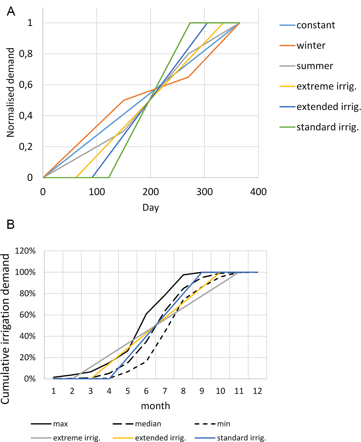
Figure 2. (a) Reference normalized cumulative demand volumes for the six types of demand considered here.
(b) Cumulative water demands over one average year: modelled demands assumed in our study and demands used in the LISFLOOD model.
Table 1. Demand patterns considered in this work.
| Name | Description | Sector represented |
|---|
| Constant
| Uniform demand along the year | Domestic water supply and several industrial and energy activities |
| Summer
| Demand higher in summer | Regions with tourism concentrated in summer |
| Winter
| Demand higher in winter: | Areas with economic activities concentrated in winter |
| Standard irrigation
| Uniform demand between May and September: | Irrigation under most common conditions |
| Extended irrigation
| Uniform demand between April and October: | Irrigation under moderately arid and warm conditions |
| Extreme irrigation
| Uniform demand between March and November: | Irrigation under very arid and warm conditions |
The schematic demand patterns in
Figure 2a are obviously a simplification but remain quite consistent with more realistic demands modelled in LISFLOOD. In the setup of the LISFLOOD model used in Bisselink et al., 2020, domestic, industrial, livestock and energy demand were represented as constant in time. Irrigation is instead computed on the basis of weather forcing.
Figure 2b shows the minimum, maximum and median among the European countries of the cumulative average monthly irrigation demands over the period 1990–2021, as represented in LISFLOOD, highlighting a good correspondence with the “standard irrigation” scheme. The irrigation demand starts earlier in Southern countries, while for Nordic and Eastern countries the irrigation period ends earlier.
Combining storage rate and total annual water availability
When total annual water availability does not change, a positive change in storage rate can be used to quantify the additional storage volume as the product of the change in storage rate and the demand volume (which must remain constant with availability – “same water, more storage needed”). Conversely, a negative change would yield the storage volume potentially no longer needed.
Availability, however, may also feature trends over the years. With the same notes of warning used for the storage rate trend, we may also describe the trend with a linear model:
[Eq. 3]
where Xy (m3) is the annual streamflow volume in the generic year y, X0 (m3) is the one in the reference year (e.g., at the beginning of the time series, 1981), sX is the trend slope (m3/year) and y is the year count from the reference year. We may have different combinations of trends in the storage rate and in water availability, as summarized in
Figure 3. For the combinations, we refer to the relative trends (i.e.
and
).
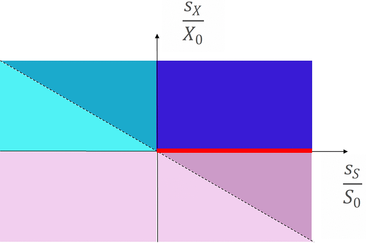
Figure 3. Classification scheme used in the analysis.
When availability increases, there is an option to increase demand. Conversely, when availability decreases we must reduce demand either by reducing water use, or by satisfying part of the demand with alternative water sources such as desalination and reuse.
The storage volume required to meet a demand is the product of demand volume and storage rate, and we assume demand always equal to availability in order to apply the mass curve analysis yearly. Hence the expected change in storage volume (or the storage volume potentially no longer needed) is the product of the change in storage rate times the change in volume available. The condition for the storage capacity to increase from year 0 to year y can be written as:
[Eq. 4]
Depending on the interplay of the trends in availability and storage rate (represented by the normalized trend slopes
and
), we may classify a river basin in terms of the action needed to adapt to changing availability and storage rate according to the scheme of
Figure 3, as explained below.
When both availability and storage rate increase (i.e.
and
), additional storage is needed if one wants to expand the demand consistent with availability (“more water, opportunity for more storage”).
When both availability and storage rate decrease (i.e.
and
), there is never a need for additional storage because the demand volume must be reduced with availability, and the latter becomes more favorably distributed in time with respect to the demand (“less water, no need for more storage”).
When availability and storage rate show opposite trends, the term
is always negative. By substituting Eq.2 and Eq.3 into Eq.4, the condition for the need of increasing storage volume can be written as:
[Eq. 5]
If the negative between the two trends is stronger than the positive
, apparently there is never a need for additional storage due to either a reduction in the available volume (as in the previous case of “less water, no need for more storage”), or a more favorable distribution of the latter in time compared to demand (“more water, no need for more storage”).
On the contrary, if the positive between the two trends is stronger than the negative
, there may be a need to increase the storage volume in the short term to satisfy the demand (“less water, need for more storage in the short term”) or to fully exploit the increased availability (“more water, opportunity for more storage in the short term”). In the long term, however, the additional storage volume becomes unnecessary because the effect of reduced availability, or the effect of a reduced storage rate, becomes prevalent. From Eq. 5, the first year when no additional storage is needed is
.
Ensemble modelling of availability
In this study, we use streamflow time series at daily steps from the LISFLOOD gridded hydrological model (Burek et al., 2013) simulated for the European scenario analysis of Bisselink et al., 2020. The model was run at a grid resolution of 5 km over continental Europe, forced with the ensemble of 11 bias-corrected climate projections from the Coordinated Downscaling Experiment - European Domain (EURO-CORDEX, see Bisselink et al., 2020) under two Representative Concentration Pathways (RCP) (Moss et al., 2008; see also Riahi et al., 2011), namely RCP 4.5 and RCP 8.5, representing a moderate and a high climate change scenario, for the period 1981–2099, for a total of 22 model simulations. Details of the model setup and more general results are provided in Bisselink et al., 2020.
From all available grid cells, we selected the cells associated with an upstream contributing area of 500 km2 or their multiples. For example, within a river basin of 1000 km2 we would have a grid cell somewhere in the middle of the catchment, and one at the outlet. This selection led to considering 4865 grid cells representing an outlet of as many river basins in Europe.
The simulated streamflow included the effect of estimated abstractions. We assume that the normalized cumulative streamflow is not significantly affected by water abstraction, i.e. it is approximately the same when computed with the natural streamflow, and with the streamflow net of water abstraction. It should be noted that we do not assume abstraction volumes to be negligible compared to streamflow volumes, but only that they do not alter significantly the intra-annual distribution of volumes, i.e., the pattern of availability.
In most European river basins, there may be a regulatory limit to abstractions when the streamflow is below a threshold of “environmental flow” (Kampa and Schmidt, 2023). To account for this restriction, we modified the simulated streamflow at each of the above outlets, by setting it to the minimum between 0 and the difference of streamflow and the “environmental flow”, thus excluding from the calculation of water availability the streamflow volume when ecosystems may be under stress. The “environmental flow” was set at 30% of the average annual flow calculated over the period 1981–2010. We checked that changing this value between 20% and 50% would not affect the results significantly (results not shown here). This somehow expected result indicates that lower flows, while ecologically important, do not influence significantly the availability of resources, hence the storage volumes required to meet the water demand patterns considered here.
Identification of trends in storage rate and availability
For each catchment outlet, climate model and the RCP, we computed the series of annual streamflow volumes, annual water availability, and annual storage rate for each of the 6 patterns of demand (see
Table 1 and
Figure 2). The slopes of the linear trend models (Eq. 2, Eq. 3) in the series of the above annual values were estimated using the well-known Theil–Sen estimator (Ohlson and Kim, 2015). Slopes not passing the Mann-Kendall test (Mann, 1945) with p = 0.05 were assumed to imply no change.
For each catchment, reference demand and RCP, we considered the average over the set of 11 slopes (one for each climate model) when these were normally distributed (Shapiro-Wilk test; Kandethody et al., 2021). In case of log-normality we transformed the values. When the 95% confidence interval of the average included 0 we assumed a zero slope. When the slopes were neither normally nor log-normally distributed, we considered the median angular coefficient instead of the average, and when not passing a sign test with p = 0.05 we assumed a zero slope. The average or median according to the above procedure was eventually retained as each catchment’s representative trend slope for subsequent analysis. These tests assured to retain trends only if robustly different from zero.
Calculation of actual water storage need
The additional storage volume required every year to meet a given demand is obtained by simple multiplication of the demand volume by the slope of the storage rate following the most appropriate pattern of demand. In the presence of various demands, each following a specific pattern, the required volumes are additive. We considered demand volumes of the domestic, industrial, energy and livestock sectors, following approximately a constant demand, and of the irrigation sector, that follows a demand higher during the summer season (
Table 1). The water demands considered are the average of years 2010–2021 as assumed in Bisselink et al., 2020 (
Table 2).
Table 2. Annual water demand for each European country in Billion m3, average over 2010–2021.
| Country | acronym | domestic | energy | industrial | irrigation | livestock |
|---|
| Austria | AT | 0.46 | 1.28 | 0.56 | 0.34 | 0.20 |
| Belgium | BE | 0.39 | 2.66 | 0.96 | 0.13 | 0.55 |
| Bulgaria | BG | 0.24 | 5.67 | 0.04 | 0.34 | 0.05 |
| Cyprus | CY | 0.12 | 0.00 | 0.02 | 0.25 | 0.00 |
| Czechia | CZ | 0.32 | 0.74 | 0.34 | 0.05 | 0.17 |
| France | FR | 3.48 | 11.98 | 2.42 | 3.99 | 1.67 |
| Germany | DE | 3.63 | 16.62 | 6.65 | 0.60 | 2.03 |
| Denmark | DK | 0.24 | 0.02 | 0.41 | 0.22 | 0.72 |
| Estonia | EE | 0.04 | 0.07 | 0.02 | 0.00 | 0.02 |
| Greece | GR | 0.79 | 0.15 | 0.25 | 11.56 | 0.29 |
| Spain | ES | 2.10 | 7.04 | 1.87 | 34.17 | 3.08 |
| Finland | FI | 0.32 | 0.57 | 0.38 | 0.06 | 0.04 |
| Croatia | HR | 0.28 | 0.17 | 0.15 | 0.06 | 0.13 |
| Hungary | HU | 0.33 | 2.95 | 0.20 | 0.27 | 0.26 |
| Ireland | IE | 0.20 | 0.40 | 0.87 | 0.00 | 0.27 |
| Italy | IT | 3.62 | 1.61 | 2.38 | 11.29 | 1.03 |
| Liechtenstein | LIE | 0.00 | 0.00 | 0.00 | 0.00 | 0.00 |
| Lithuania | LT | 0.07 | 0.05 | 0.04 | 0.00 | 0.09 |
| Luxemburg | LU | 0.03 | 0.00 | 0.04 | 0.00 | 0.01 |
| Latvia | LV | 0.10 | 0.01 | 0.02 | 0.00 | 0.01 |
| Malta | MT | 0.01 | 0.00 | 0.01 | 0.01 | 0.00 |
| The Netherlands | NL | 0.76 | 1.50 | 1.02 | 0.16 | 0.78 |
| Poland | PL | 1.27 | 5.91 | 0.71 | 0.08 | 1.26 |
| Portugal | PT | 0.57 | 0.19 | 0.24 | 2.18 | 0.45 |
| Romania | RO | 0.87 | 2.08 | 0.31 | 2.06 | 0.48 |
| Sweden | SE | 0.54 | 0.25 | 1.54 | 0.11 | 0.06 |
| Slovenia | SI | 0.07 | 1.15 | 0.06 | 0.01 | 0.02 |
| Slovakia | SK | 0.15 | 0.17 | 0.13 | 0.09 | 0.08 |
| European Union | EU | 20.98 | 63.23 | 21.64 | 68.03 | 13.77 |
| Norway | NO | 0.82 | 0.01 | 0.52 | 0.08 | 0.05 |
| United Kingdom | UK | 3.45 | 0.60 | 2.73 | 0.08 | 0.69 |
| Switzerland | CH | 0.99 | 0.35 | 0.70 | 0.08 | 0.15 |
We computed the weighted average of storage rate trend slopes ss across the river basin outlets in each European country for each sector’s demand. For a more conservative estimate, we consider only the basins where
ss,k > 0, i.e. with increasing storage need, while clearly part of the demand may be in river basins with constant or decreasing requirements. The additional volume for a country for each demand is calculated for the c-th country as
, where Nc is the number of river basins considered in the country and Dc is the annual demand in the country. The sum of domestic, energy and industrial annual demands was multiplied by the weighted average of storage rate trend slopes ss of the constant demand, winter demand and summer demand, obtaining three values of storage volumes and keeping the minimum, the maximum and the median one among the three. Irrigation demand was multiplied by the three slopes ss corresponding to standard, extended and extreme irrigation demands, obtaining again three values and keeping the maximum, median and minimum. Finally, the storage volumes are summed together to obtain the overall minimum, median and maximum additional storage requirements.
3. Results
Figures 4 and 5 show the European distribution of trend in storage rate (ss) and annual water availability (sx) under RCP 4.5 and RCP 8.5, respectively.
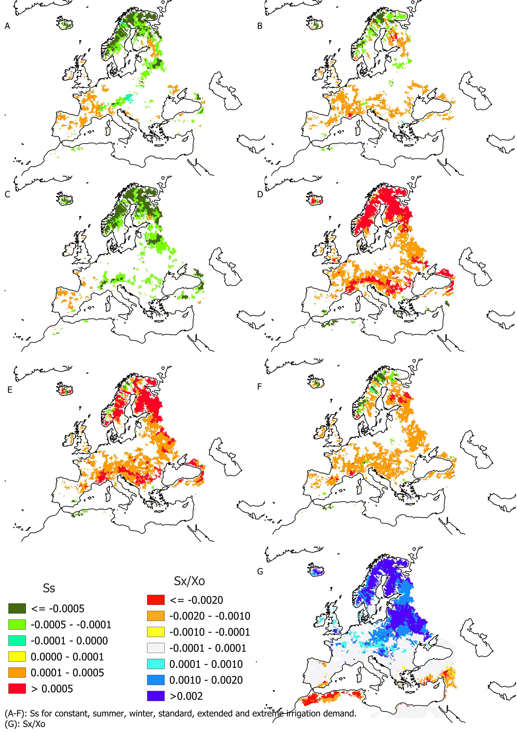
Figure 4. Slope of normalized storage volume for A) constant demand, B) summer demand, C) winter demand, D) standard irrigation demand, E) extended irrigation demand, F) extreme irrigation demand.
Pane G) shows slope of availability. All are calculated under RCP 4.5.
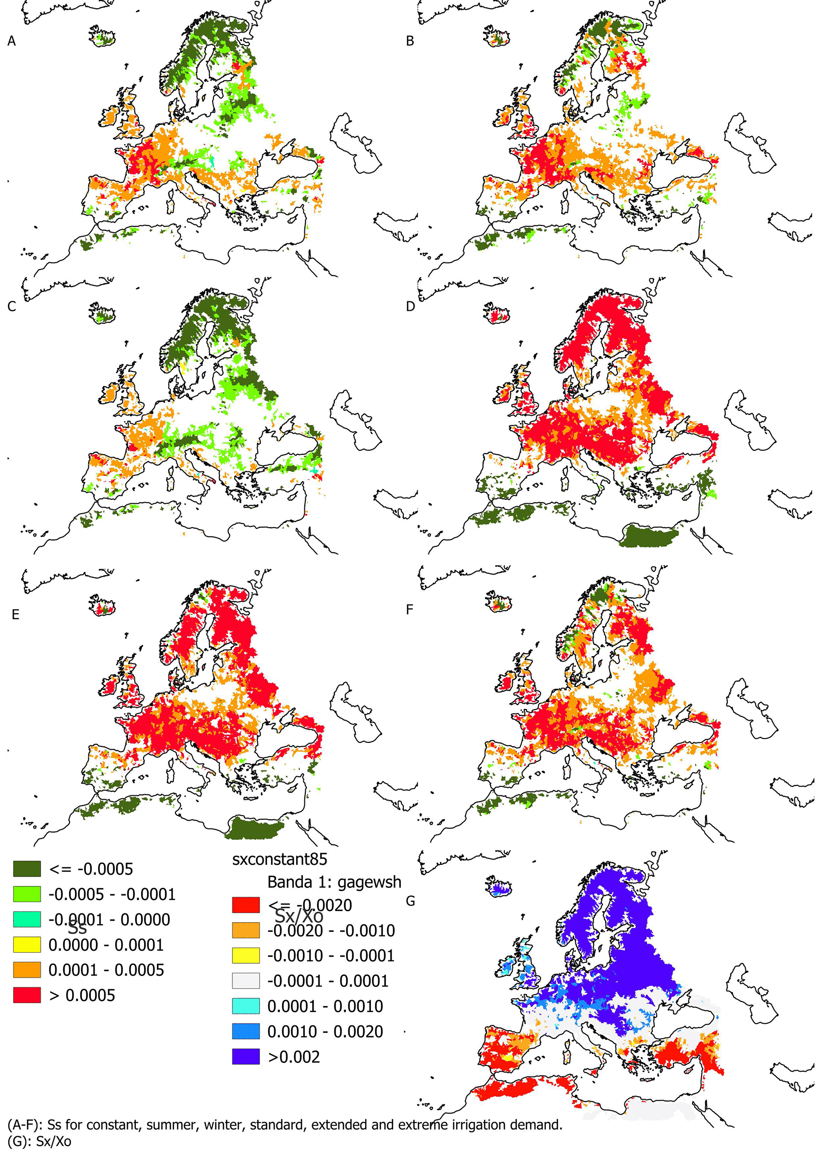
Figure 5. Slope of normalized storage volume for A) constant demand, B) summer demand, C) winter demand, D) standard irrigation demand, E) extended irrigation demand, F) extreme irrigation demand.
Pane G) shows slope of availability. All are calculated under RCP 8.5.
Availability (
Figures 4(G) and 5(G)) presents negative trends in southern Europe and the Mediterranean, positive trends in northern and north-eastern Europe and a central transition zone, where a clear trend cannot be defined with sufficient confidence. The pattern is the same for scenarios of RCP 4.5 and RCP 8.5, although apparently more pronounced in the latter. Particularly, in southern Europe a clear negative trend in availability emerges mostly under RCP 8.5 while under RCP 4.5 the trend seems less significant. The more negative the trend, the higher is the need to put in place measures to reduce demand or to resort to non-conventional sources (such as desalination and/or water reuse).
For storage rates, patterns appear more complex. Under RCP 4.5, we find that for a constant demand and a demand higher in winter there is a negative trend in required storage rates for central and northern Europe, and no or only weakly positive trends in the south of the continent (
Figure 4(A), (C)). The required storage rates for irrigation demand (
Figure 4 (D), (E), (F)) show widespread positive trends, in line with the projected lower water availability in summer. The required storage rates for demands concentrated in summer (
Figure 4(B)) show a pattern in between the two above. Under RCP 8.5 (
Figure 5), the patterns are similar but more pronounced: the required storage rates for constant demand show widespread positive trends in the west and south of Europe (
Figure 5(A)). A negative trend indicates that the temporal distribution of water availability along the year tends to become more in phase with the demand, implying less need for storage if the total cumulative demand does not change. On the contrary, a positive trend implies that, the need for storage increases as availability becomes more staggered with respect to demand. However, in many cases the trend in availability combines with the trend in storage rate, and we apply the interpretation scheme of
Figure 3 to classify the river basins (
Figure 6 and
Figure 7).
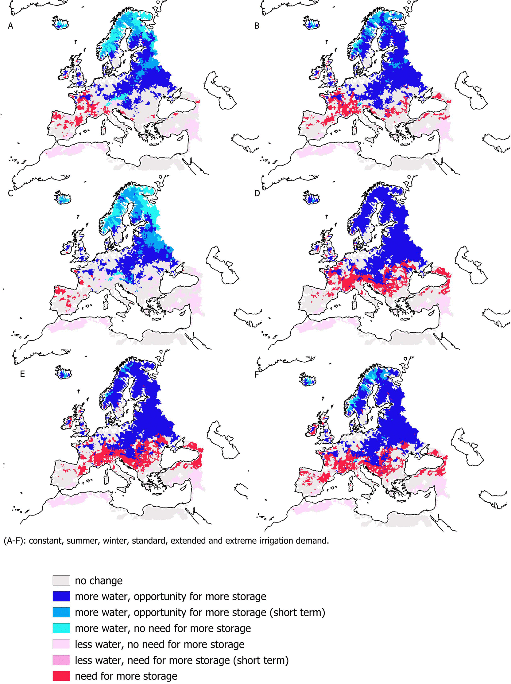
Figure 6. Classification of river basins following the scheme of
Figure 2, for A) constant demand, B) summer demand, C) winter demand, D) standard irrigation demand, E) extended irrigation demand, F) extreme irrigation demand, for RCP 4.5.
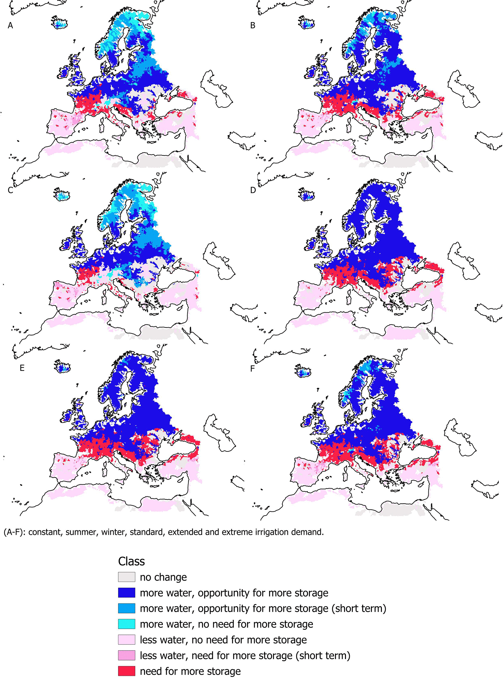
Figure 7. Classification of river basins following the scheme of
Figure 2, for A) constant demand, B) summer demand, C) winter demand, D) standard irrigation demand, E) extended irrigation demand, F) extreme irrigation demand, for RCP 8.5.
The classification depends on the type of demand that we consider.
Figure 6 and
Figure 7 present the results for RCP 4.5 and RCP 8.5, respectively, with blue indicating opportunity for additional water storage to exploit the increasing water availability, red indicating need for water storage to cope with availability less in phase with demand, and paler colour tones indicating less or no need or opportunity for additional storage. The patterns in
Figure 6 and
Figure 7 are rather similar and highlight how in the north of Europe there is an opportunity for more storage in order to harvest more water available, and in the south there is generally no need for more storage as the reduction of availability is predominant. The patterns are more pronounced when considering demands concentrated in summer (cases (B), (D), (E), (F) in
Figure 6 and
Figure 7) and generally under RCP 8.5 (
Figure 7) compared to RCP 4.5 (
Figure 6).
Tables 3 and 4 show the correlation matrix of the trend in intra-annual storage, sS, in each pixel under the combination of different demands, and how many catchments (in % on the total number of 4865) have the same classification under different demands, considering RCP 8.5.
Table 3. Correlation matrix of the slopes sS, RCP8.5.
| Const | Irr_extend | Irr_extr | irr_std | winter | summer |
|---|
| Const
| 1.00 | | | | | |
| Irr_extend
| 0.01 | 1.00 | | | | |
| Irr_extr
| 0.55 | 0.77 | 1.00 | | | |
| irr_std
| −0.28 | 0.87 | 0.48 | 1.00 | | |
| Winter
| 0.91 | −0.25 | 0.30 | −0.48 | 1.00 | |
| Summer
| 0.79 | 0.50 | 0.85 | 0.23 | 0.59 | 1.00 |
Table 4. Pixels with the same classification, RCP8.5.
| Const | Irr_extend | Irr_extr | irr_std | winter | summer |
|---|
| Const
| 1 | | | | | |
| Irr_extend
| 58% | 1 | | | | |
| Irr_extr
| 64% | 87% | 1 | | | |
| irr_std
| 54% | 91% | 82% | 1 | | |
| winter
| 84% | 50% | 56% | 47% | 1 | |
| summer
| 77% | 71% | 78% | 67% | 67% | 1 |
The results associated to the constant demand are correlated with those of the summer and winter demands (correlation coefficient above 0.8) and most of the pixel (around 80%) have the same classification. The extended irrigation demand, which is in the middle of the extreme and standard demands, is correlated well with these two, while the extreme and standard demands show a less correlated behaviour. The extreme irrigation is correlated well with the summer demand. The winter demand is less correlated with the others, except with the constant demand, which is quite intuitive, as it is the only one with prevalent water withdrawal in wintertime. Therefore, the results could be presented by showing just 3 demands: the constant one (representative of the winter one too), the summer one (representative of the extreme too), and the extended or the standard one.
It is noteworthy how, in a central belt of the continent, positive trends in storage rates combined with no trend in availability indicate a need for additional storage volume to meet the current demand.
From indicator sS (slope of the intra-annual storage rate trend in time), we can estimate the additional storage volume required to meet a given demand at a certain year y, as described in section 2.6.
Figure 8 shows the median and range of additional volume for the different European countries, resulting from considering the 6 types of demand, under the RCP 8.5 scenario (volumes under RCP 4.5 are lower and not further discussed here). The required increase in storage volume ranges from 72 Mm3 to 110 Mm3 per year for the whole of Europe (median is 88.7 Mm3), or 7 to 11 billion m3 over a century. This is a small volume compared e.g. with the 365 billion m3 storage capacity of the 5,575 European large dams, or 280 billion m3 of the ca. 4,500 reservoirs of the EU’s large dams, according to the World Register of Dams of the International Commission on Large Dams (ICOLD, 2023). The countries with the largest need in absolute terms are Germany (7.3–14.8 Mm3/y, which corresponds to 0.17%–0.34% of large reservoirs’ volume in the same country), Spain (20.1–22.9 Mm3/y, i.e., 0.027%–0.028%), France (9.4–15.0 Mm3/y, i.e., 0.07%–0.11%) and Italy (9.8–13.7, Mm3/y, i.e., 0.017%–0.019%). In terms of percentage of the total existing storage volume of large dams (ICOLD, 2023), Belgium (0.77%–1.45%), Germany (0.17%–0.34%), Hungary (0.57%–0.59%) and Slovenia (0.15%–0.28%) are those with the largest relative needs. Italy, Greece, Belgium and the Netherlands show the largest volumes relative to the country surface area (mm or thousand m3 per km2 -
Figure 8).
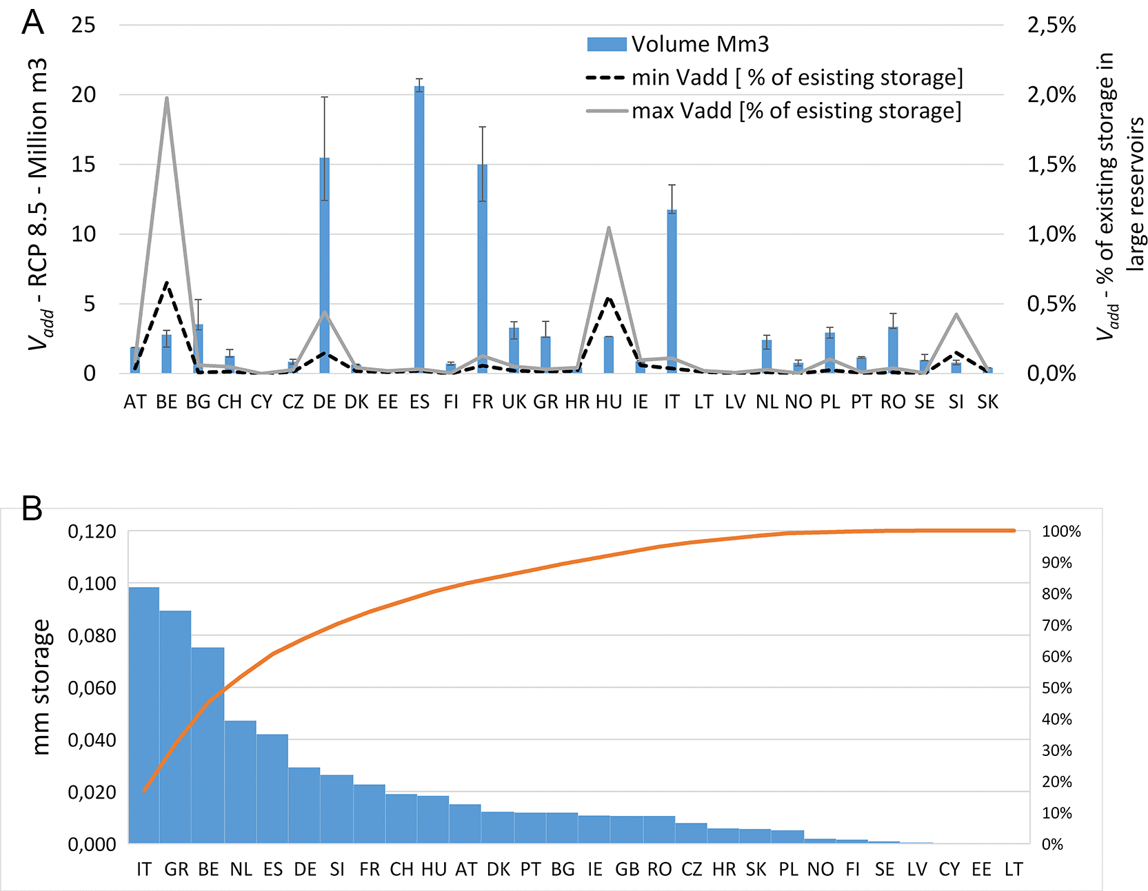
Figure 8. (A) Additional water storage volume per year required in European countries (EU plus Switzerland (CH), UK and Norway).
Blue and error bars represent the median value, minimum and maximum value, considering the six different demands for RCP 8.5, and the lines the % of the minimum and maximum volume to the existing storage capacity in artificial reservoirs; (B) water storage relative to country surface area.
4. Discussion
By analyzing the two complementary trends in total available streamflow volume and in intra-annual storage capacity need, reflecting the distribution of availability with respect to demand, we have identified conditions requiring different adaptation strategies to cope with climate change: a reduction of demand under lower availability, and an increase of storage capacity when availability is less in phase with demand. Many cases also require a combination of the two. When availability increases, there is even an opportunity to increase demand, often at the cost of additional storage.
Although the design of interventions requires a more specific quantitative analysis, our analysis supports strategic planning towards adaptation and resilience. The indicators proposed here can be used to estimate additional storage volume requirements and demand reduction targets to cope with climate change, which represent key information in support to adaptation plans and the programming of investments.
Decreasing trends in annual water availability indicate a widespread need for water use efficiency, water saving measures, and alternative water resources (Christou et al., 2024; Molinos-Senante et al., 2016; Pistocchi et al., 2018; Pistocchi et al., 2020; Quaranta et al., 2023; De Roo et al., 2023) in several regions in Europe. The additional storage volumes required to cope with changes in variability over the next century, on the contrary, seem rather small (a small or very small percentage of the current storage capacity). These additional volumes correspond to the average trend across 11 climate models. If we consider the maximum trend instead of the average (or median), i.e. the worst-case model, we obtain volumes higher by a factor of approximately 2 (results not shown here for simplicity). This would still be a relatively small additional storage (between about 14 and 22 billion m3 in the next century). A further test using the trend in the mobile 9-year maximum of annual storage rates did not highlight appreciable differences compared to the trend in simple annual storage rates (results not shown here). We must stress that relatively small variations in intra-annual storage volume may conceal a more significant demand for inter-annual compensation due to changing sequences of drought and wet years. Moreover, even if the increase in required intra-annual storage volume may seem small, it is by no means negligible: it is equivalent to building a few large dams every year across Europe, a densely populated context where the most suitable locations are already exploited, and where the demand for nature restoration and conservation is very high. The periglacial Alpine environment could offer among the few opportunities still available for new reservoirs at lower environmental impact (Farinotti et al., 2016; Farinotti et al., 2019). The volumes needed to address the trends detected through climate model simulations could be also in part obtained through the optimization of operation and maintenance of existing reservoirs (Gimeno-Gutiérrez and Lacal-Arántegui, 2015; Fauriel et al., 2023; Quaranta et al., 2021a; Panagos et al., 2024), or through other forms of storage such as managed aquifer recharge (e.g. Pyne, 2017, Varouchakis et al., 2023), use of abandoned mines and quarries (Ordóñez et al., 2012; Weber et al., 2024), better soil management, or nature-based solutions including urban greening (Quaranta et al., 2021b; Quaranta et al., 2022). This strengthens the case for consistent and coordinated planning of interventions at least at the regional scale, even if limited to the volumes quantified here. Our analysis identifies also river basins with negative trends in storage rates, hence a possibility to reduce water storage capacity. In these cases, dam removal could be an option to restore free flowing rivers and river longitudinal connectivity, as requested by the Nature Restoration Law (European Commission, 2024), with due consideration for the ecological, socioeconomic and water security implications (see e.g. Stanley and Doyle, 2003; Sneddon et al., 2017).
5. Conclusions
We proposed an approach to extract information directly applicable to support adaptation strategies at the regional scale from complex model simulations, based on the use of indicators including the newly proposed “storage rate”. We have suggested criteria for the planning and programming of adaptation measures in Europe through storage, demand reduction, or a combination of both. The analysis may offer support also in the development of strategies to increase the resilience of specific economic activities, within the limits of validity of hydrological simulations of climate change scenarios. This contribution offers a screening of the needs for additional water storage and water demand management. In line with the EU Water Resilience Strategy (EC, 2025), water storage should prioritize nature-based solutions, while the planning of new dams and reservoirs should carefully evaluate their environmental impacts, in the context of an integrated and sustainable water management strategy informed by climate projections to avoid stranded investments. Our approach does not replace more detailed analyses, but allows a quick interpretation of complex model scenarios and a first screening-level assessment of adaptation requirements for regional strategic planning.
Ethics and consent
Ethical approval and consent were not required.