Introduction
NEXT – New Exploration Technologies – was a Horizon 2020 project funded by European Union in 2018–2021. NEXT developed new geomodels, novel sensitive exploration technologies and data analysis methods, which together are fast, cost-effective, environmentally safe and potentially more socially accepted. The project was built on three pillars of technological advances: (1) mineral systems modelling, (2) exploration methods and approaches, and (3) data processing and data integration tools. The NEXT consortium was coordinated by the Geological Survey of Finland (GTK) and consisted of 16 partners from research institutes, academia, service providers and mining industry from the six EU member states Finland, Sweden, Germany, France, Malta and Spain, who represented the main metal-producing regions of Europe.
Geophysical electromagnetic (EM) methods are commonly used in geological mapping, mineral exploration, groundwater studies and geotechnical investigations. Compared to ground surveys, airborne EM methods have the benefit of avoiding terrain obstacles such as lakes, rivers, swamps, and ravines. Compared to manned aircrafts, drones or unmanned aerial vehicles (UAVs) have benefits of their own. Drone-based surveys are versatile, fast to deploy, economical and ecologically more friendly. Unlike the instruments used to measure magnetic field, EM devices tend to be quite heavy, and hence, are not well suited for drone-based applications. Moreover, systems based on EM induction utilize separate transmitter and receiver units and the power of the EM transmitter is directly proportional to the maximum depth of investigation. In other words, heavy EM equipment is needed to be able to investigate deeply situated targets.
Yet, drones can be highly useful in the mapping of the geoelectrical properties of the near-surface (0–100 m) parts of the earth. In the NEXT project, Radai Ltd developed a novel geophysical EM survey system (Louhi) for practical drone-based operations. Similar light-weight frequency-domain EM systems do not yet exist on the market. This paper presents theoretical background of geophysical EM applications, Radai’s solution to drone-based EM surveying and gives examples from the first tests made with the Louhi EM system.
Theory of geophysical electromagnetic methods
Background
Geophysical research methods such as seismic, magnetic, gravimetric, electrical (dc) and electromagnetic (ac) methods are used to retrieve information on the structure and composition of the subsurface materials indirectly, i.e., without disturbing the target of interest. This is accomplished by measuring changes in the intensity of physical force fields (e.g., electric potential or magnetic field). The force fields may be of natural origin (e.g., magnetic and gravimetric field) or they can be generated by man (e.g., electromagnetic or seismic sources). The changes in the measured field are caused by changes in the petrophysical properties (e.g. electrical conductivity, magnetic susceptibility, density, seismic P-wave velocities) of the subsurface materials due to changes in the mineral and material content and texture of the subsurface. Thus, by mapping the changes in the force fields, it is possible to remotely map the changes in the geological materials inside the earth. Moreover, some geophysical methods (e.g., electromagnetic and seismic methods) can be used to determine not only lateral changes (geological contacts) but also the depth variation and optimally even the 3D structure of the subsurface. Generally, however, multi-dimensional interpretation of the geophysical data requires numerical inversion software.
EM theory
The theory of geophysical electromagnetic methods can be described by Maxwell’s equations (Maxwell, 1892a; Maxwell, 1892b and Ward & Hohmann, 1988):
where E is the intensity of the electric field (V/m), B is magnetic flux density (magnetic induction, Vs/m2 = T), H is the intensity of magnetic field (A/m), D is dielectric displacement (C/m), J is electric current density (A/m2), and ρ is electric charge density. E, D, B, H and J are vectors with amplitude and direction, whereas ρ is a scalar quantity (having amplitude only). All quantities are functions of position (r) and time (t).
Faraday’s induction law, Equation (1), says that a time-varying magnetic field generates an electric field around it. Ampère-Maxwell’s law, Equation (2), says that static current flow generates a magnetic field around it. Equation (3) manifests the conservation of charges and that electric field is caused by free charges. Equation (4) states that magnetic charges do not exist (magnetic field is caused by electric field).
The constitutive equations that combine the different vector quantities and connect them with the physical properties of earth materials are (Ward & Hohmann, 1988):
where the three petrophysical properties of the media are: ε = dielectric permittivity (As/Vm), μ = magnetic permeability (Vs/Am), and σ = electric conductivity (S/m = A/(Vm)). For the sake of simplicity, the media (air, soil, rocks) are considered to be linear, isotropic and homogeneous. This means that ε, μ and σ are scalar quantities that do not depend on any other parameters (temperature, pressure), frequency or time (no dispersion) and direction (no anisotropy).
Often the magnetic properties of the media can be ignored (μr = 1) and the magnetic permeability is assumed to be equal to that of free space μ = μrμ0 = 4π·10-7 (Vs/Am) everywhere. If geological targets have high magnetic susceptibility (χ=μr-1) and low conductivity, this assumption is no longer valid and should require special attention. In addition, since we are dealing with low frequency EM fields, the dielectric properties can be ignored too (εr = 1) and dielectric permittivity is assumed to be equal to that of free space ε = εrε0 ≈ 8.8542·10-12 (As/Vm). This assumption is not valid for high frequency EM methods (e.g. ground penetrating radar (GPR) and radio-EM) where the wave nature of EM fields needs to be taken into account. For low frequency (inductive) EM methods, however, the diffusion of the EM fields is the most important physical phenomenon. Because of this, the resolving capabilities of low-frequency EM methods is not as good as that of high-frequency methods.
Basics of EM applications
The principles of geophysical EM methods are illustrated in Figure 1.
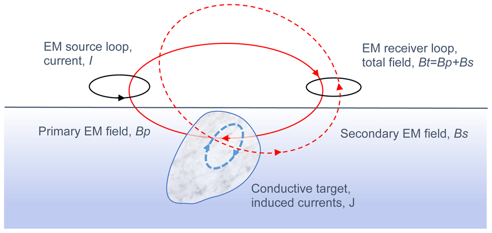
Figure 1. Principles of geophysical inductive electromagnetic (EM) methods.
The solid red line depicts imaginary force lines of the primary field (Bp), dashed blue line depicts induced currents (J) and the dashed red line depicts secondary EM field (Bs).
1. The electric current of the EM source creates a primary magnetic field (solid red line, Bp) around it according Equation (2). Since the current is time-varying, the magnetic field is too.
2. The time-varying magnetic field has an induced electric field (E) around it according to Equation (1).
3. In a conductive medium (σ > 0) the electric field builds up current density (dashed blue line, J) according to Equation 7 (Ohm’s law).
4. The induced currents (J) are the source of the secondary magnetic field (dashed red line, Bs) according to Equation (2).
5. The EM receiver measures the total field (Bt), i.e., the sum of primary and secondary fields (Bt= Bp+Bs).
By moving the transmitter and the receiver over the surface, the coupling between transmitter, conductor and receiver changes, which in turn, changes the EM response. Due to geometric attenuation of the EM fields, the changes in the response are strongest close to the conductors. Any sign reversals in the response are also very informative. Numerical modelling and inversion are needed to interpret the EM data of complex 3D structures.
Electromagnetic methods can be divided into frequency-domain (FEM) and time-domain (TEM) methods (Swift, 1988). The division is made based on the transmitter waveform, which in FEM methods is time-harmonic (I= I0sin(ωt), I0 is the peak amplitude of the current and ω=2πf is angular frequency in radians and f is frequency in hertz) and measurements are made as a function of measurement frequency. In TEM methods, the source field is usually an EM impulse generated by an abrupt change (turn-off and turn-on) in the current and the measurements are made as a function of time after the EM impulse. The benefit of TEM methods is that the response is measured in the absence of the primary field which is normally much stronger than the secondary field. Consequently, TEM methods have better signal-to-noise (SNR) ratio and deeper exploration depth than FEM methods particularly in conductive surroundings (Swift, 1988). The benefit of FEM methods is that the frequency (or frequencies) of the primary field is known in advance and it is possible to design the electronics of the measurement device and data post-processing based on that knowledge (Swift, 1988). Consequently, FEM methods are more sensitive to low conductivity targets. Since the new EM method developed in the NEXT project is a frequency-domain method, TEM applications are not discussed in this paper any further.
The frequencies used in FEM applications typically range from 10 Hz to 20 kHz. Due to the attenuation of the EM fields in conductive medium, the lower the frequency is, the deeper into the ground the EM field can penetrate before reducing in amplitude so much that the secondary field of the induced currents cannot be separated from noise. The EM attenuation is defined by skin depth, which represents a distance during which the intensity of EM plane-wave reduces by 1/e (≈ 37%) inside homogeneous conductive medium (Ward & Hohmann, 1988).
where ω= 2πf, is the angular frequency. Considering FEM methods, however, the lower the frequency is the lower is the voltage induced to the receiver (cf. Equation 1). Consequently, the SNR reduces making it impossible to separate the secondary field from the EM noise. To some degree the noise can be reduced by repeating the measurements several times and averaging the response. This works nicely for a ground EM system that just needs to stay at a fixed position a bit longer. Considering a moving EM system, however, the time spent during the process of averaging creates unwanted spatial smoothing of the EM response and, in practice, it means that the minimum frequency needs to be set higher for a moving EM system.
EM transmitters
With the exception of the methods utilizing natural EM fields (e.g., magnetotelluric method) and some special systems like the very-low frequency (VLF) EM method, the most common transmitters are 1) a small loop of insulated metal wire, i.e., a magnetic dipole, 2) a large loop of wire, 3) a long straight wire grounded at both ends.
The larger the surface area (A) of the transmitter loop is, the stronger is the transmitter moment (M=NIA) and the strength of the primary EM field. In ground EM studies the loop area can be up to 1 km by 2 km (2·106 m2). The longer the wire needed for the large loop, the higher is its resistance, and hence, the smaller is the current. Furthermore, moving and setting up a large loop takes more time and effort. Operating a small transmitter loop is more practical, but the smaller the loop is, the greater is the geometric attenuation of the EM field (from 1/r3 for dipole to 1/r for long straight wire). Ideally, a large loop laid out on the ground (and operating at low frequency) gives the maximum depth of exploration.
Usually the current amplitude (I) is a few amperes (1-10 A) and the number of loop windings (N) varies from a single turn to a few hundreds of turns. Increasing the number of loop windings increases the (self)inductance of the loop which reduces the maximum current and transmitter moment. To counteract this, the transmitter can be tuned up using a suitably chosen capacitor.
Since both the depth of exploration and data resolution depend on the frequency (e.g., Spies & Frischknecht, 1991), broadband multi-frequency EM systems give more information than single frequency systems that suit mainly just for geological mapping, i.e., delineating conductivity boundaries. However, utilizing several frequencies increases the measurement time because more data samples need to be gathered to reach good data quality. In principle, it is possible to create a multi-frequency EM system where all the frequencies are transmitted at the same time. Whether this is possible or not depends on the type of EM receiver and data collection unit. For the same reasons as for data averaging, the number of frequencies cannot be increased without increasing the measurement time. For a moving EM system this means that the number of frequencies that can be collected at the same time is limited.
EM receivers and system geometry
Various different types of EM receivers exist (e.g., Spies & Frischknecht, 1991). The two most commonly used receivers are 1) a loop of insulated metal wire and 2) an induction coil that both measure the voltage or current induced in them. According to Faraday’s law (Equation 1), the induced voltage is related to the time derivative of the magnetic flux density (dB/dt). Alternatively, the electric field (E) can be measured directly by measuring the voltage (V) between two grounded electrodes. If the frequency is not too high, a (flux gate or squid) magnetometer can be used to measure the intensity of magnetic field (B) directly.
Usually, the receiver measures a single component of the EM field that is either maximum or minimum coupled with the transmitter field. Maximum coupling means that the receiver axis is parallel to the normal of the transmitter loop or its primary field at receiver position. Minimum coupling means that the axis of the receiver is perpendicular to the primary field. In practice, reaching the minimum coupling is difficult unless both the transmitter and the receiver are built into a fixed frame.
One of the most common EM system geometries is the horizontal loop EM system (HLEM a.k.a. Slingram), where the transmitter is a small horizontal loop (vertical dipole axis), the receiver is a horizontal loop or a coil (vertical axis) and the distance between the transmitter and receiver is kept constant while the system is moving (Frischknecht et al., 1991). This system has the advantage that it is also sensitive to conductive layers in the earth (Swift, 1988). The two low-altitude airborne EM (AEM) systems used by Geological Survey of Finland (GTK) utilized coaxial vertical loops (VCA), where the source and receiver were at the tail and nose of the airplane, and vertical coplanar loops (VCPL), where the transmitter and receiver loops were at the end of both wings (Peltoniemi, 2005). Vertical loop systems have the advantage that they are sensitive to vertical conductors in the earth (Swift, 1988).
By using three orthogonal receiver loops, coils or electrodes, all the three components of the EM field can be measured. Naturally measuring the vertical component of the electric field is a bit of a challenge and in practice never done. Taking full advantage of a three-component receiver means that either its orientation (e.g., roll, pitch, and yaw) is measured also or the receiver is carefully oriented before making the measurements.
EM responses
The frequency-domain EM response can be defined in numerous different ways (e.g., Spies & Frischknecht, 1991). Depending on the receiver, the response can be defined simply as the measured quantity (e.g., the voltage or the intensity of magnetic field). However, numerical modelling of such data is more or less impossible unless the receiver is calibrated using a known external field. Calibration also provides a method to transform measured voltages into values of magnetic field or flux density. Frequent calibration is needed if the (electrical or physical) properties of the receiver do not stay the same from day to day.
The amplitude of the EM primary field greatly varies as a function of distance between the transmitter and receiver. Therefore, and to help visual data interpretation, the EM response is often defined as a normalized quantity (Spies & Frischknecht, 1991). Most commonly the measured total field is divided by the primary (free-space) field at receiver location (e.g., Bz/Bz0). In case of a three-component receiver, each measured field component is first rotated to XYZ (east, north, up) or NED (north, east down) coordinates and then normalized with the total intensity of the primary field (e.g., Bx/B0, By/B0 and Bz/B0). Unless the EM system is fixed, computation of the normalized response requires that 1) the transmitter current, 2) the distance between the transmitter and receiver as well as 3) the orientation of the source and receiver is known in advance and/or measured along with the EM data. For EM systems with a fixed geometry, the latter two conditions are easy to meet but for an UAV based EM system, they cause an additional complication.
At this point, it is important to mention that the frequency-domain EM response is a complex quantity. In other words, the EM response is defined either using real (Re) and imaginary (Im) components or amplitude (A) and phase (φ) components (e.g., Spies & Frischknecht, 1991). The real and imaginary parts are also known as the in-phase (IP) and quadrature (Q) components, which imply that the real component is the amplitude of the EM field that is in the same phase as the primary field and the imaginary component is 90 degrees behind.
The concept of FEM response is illustrated in Figure 2. The graphs on the left depict the time delays (phase shifts) between primary magnetic field (Bp), EM induction (electromotive force), secondary field (Bs) and total field (Bt= Bp+Bs). The figure on top right depicts the primary, secondary, and total fields in a phasor diagram, where horizontal axis is the real (in-phase) component and vertical axis is the imaginary (quadrature) component. The other graphs on the right depict the phase shift between primary field and total field and the concept of dividing the field components into real and imaginary parts which are in phase and in quadrature with the primary field, respectively. The angle (α) between primary and total field is a phase difference that can be measured if the time difference between the peaks of the total field and primary field (or current) is known. The secondary field has a phase shift of 90 degrees because of induction (dB/dt) and an additional phase shift (φ) due to propagation and EM interaction in conductive material. By dividing the secondary field into real and imaginary parts the amplitude and the phase of the secondary field can be computed easily as A= (Re2+Im2)1/2 and φ= arctan(Im/Re). Moreover, the normalized response can be defined as Re= Re(Bt/Bp)-1 = Re((Bp+Bs)/Bp)-1= Re(Bs/Bp) and Im= Im(Bt/Bp)= Im((Bs+Bp)/Bp)= Im(Bs/Bp), since primary field has no quadrature component (Im(Bp)= 0).
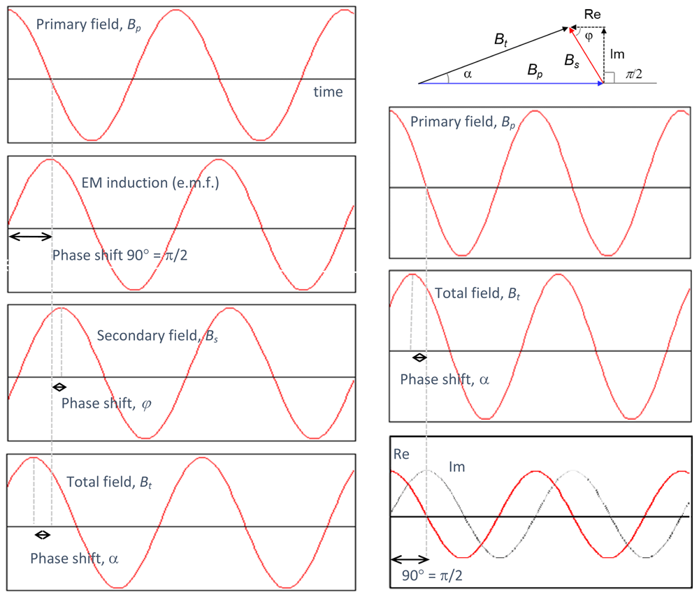
Figure 2. Definition of frequency-domain electromagnetic (EM) response.
The graphs on the left depict phase delays between primary field (Bp), EM induction, secondary field (Bs) and total field (Bt). The graphs on the right define the real (in-phase) and imaginary (quadrature) components of the EM response.
One very useful type of EM response is the ratio between vertical (Bz) and horizontal (Bh), or more precisely, the radial component (Br) of the measured response. Due to geometric attenuation of fields and different attenuation rates of vertical and horizontal fields over conductive earth, the Bz/Br-ratio can be used in 1D inversion to determine the apparent conductivity of the medium. If multiple frequencies are used, 1D inversion using a layered earth model is also possible. The benefit of using the Bz/Br-ratio lies in the fact that the exact phase, i.e., the time synchronization with the transmitter current, is not needed. This helps system development as it makes it possible to utilize the measured data before the time synchronization is even implemented.
Radai’s drone-based EM system, Louhi
Main concept
The new EM survey system comprises a single drone carrying a 3-component EM receiver and an EM transmitter which is either 1) a small (radius < 1 m) moving loop carried by another drone or 2) a large loop of current (size > 50 m by 50 m) laid on the ground surface (Figure 3). In the latter system, the EM receiver unit flies over the survey area along a system of survey lines in the neighborhood of the EM transmitter (distance <2 km). In the 2-drone system, both the transmitter and the receiver are flown along the survey lines either in an inline/tandem (one after another) or broadside (side by side) fashion while keeping the distance between them approximately the same (loop separation, L<50-200 m).
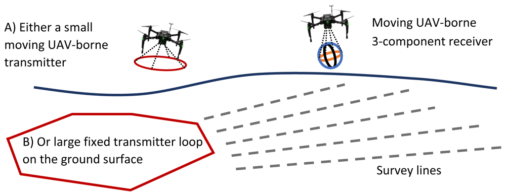
Figure 3. The concept of unmanned aerial vehicles (UAV) based electromagnetic (EM) survey method.
The EM primary field is generated either by A) a small moving current loop carried by a drone or B) a large loop laid on the ground surface. In both cases, the EM response is measured with a 3-component receiver carried by another drone.
The benefit of a fixed loop transmitter is the bigger source moment (M= NIA) due to the larger surface area (A) of the loop, and hence, better signal-to-noise ratio (S/N) and deeper depth of exploration compared to moving loop systems (e.g., Spies & Frischknecht, 1991). Fixed loop is also beneficial in the development work and testing of the EM receiver unit as it provides a constant source field. In practice, the location of the fixed transmitter loop with respect to subsurface conductors needs to be carefully planned, and possibly, the measurements need to be repeated using different source locations to illuminate/energize the conductive target(s) from another direction. Considering that setting up the transmitter cable can be time-consuming in rugged terrain, large loop systems are not well suited for reconnaissance work and/or under unknown geological settings.
The benefit of using a two-drone system is that the terrain obstacles (trees, rivers, lakes, swamps, fences) do not hinder, or even worse, totally prevent surveying. Being fully airborne, the two-drone system can be deployed quickly and suits reconnaissance work better than fixed loop systems. Moreover, the freely adjustable loop separation (L= 50-200 m) provides a method to adjust the depth of exploration based on the conductivity/resistivity of the particular study area (Spies & Frischknecht, 1991). In principle, hand-held EM devices (e.g., Geonics EM-31 or Geophex GEM-2), in which the transmitter and receiver are built onto a rigid frame, could be carried by a single drone, but due to their small size and weak transmitter moment their applicability is limited, particularly, if they are to be operated above the height level of tree-tops (30-50 m).
The two-drone system has several caveats, however. The variation in the loop separation and the variation in the transmitter and receiver orientation (roll, pitch and yaw) make the raw data appear very noisy. Figure 2 illustrates the parameters of the two-loop EM system. By accurately measuring the (x,y,z) position of both the transmitter (tx,ty,tz) and receiver (rx,ry,rx) and their orientation (rt,pt,yt and rr,pr,yr), the measured data (Hx’,Hy’,Hz’) can be converted to global 3D coordinates (see Figure 4), the corrected data (Hx,Hy,Hz or Hr,Hz) can be used in EM inversion, and the variations in the primary EM field can be modelled appropriately. In other words, despite the noisy appearance of the data, post-processing can yield informative results, such as apparent resistivity and/or resistivity pseudo-sections, that are free from the noise arising from changes in the measurement geometry. In case of a fixed-loop transmitter, the amount of noise is less as the vertices of the loop (vx,vy,vz) are fixed.
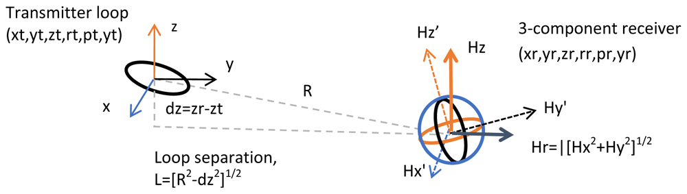
Figure 4. The parameters of a two-loop electromagnetic system.
(xt,yt,zt) refer to XYZ coordinates of the transmitter and (xr,yr,zr) refer to those of the receiver. (rt,pt,yt) refer to roll, pitch and yaw angles of the transmitter and (rr,pr,yr) to those of the receiver. (Hx’,Hy’,Hz’) are the three measured components of the magnetic field in device coordinates and (Hx,Hy,Hz) are the (away from transmitter) components of the magnetic field in world coordinates.
The time synchronization between the transmitter current (or primary EM field) and the measured data (Hx,Hy,Hz) plays an important role in the new EM system. In traditional ground and airborne EM systems, the zero phase of the current is known because there can be a cable between the transmitter and receiver. In Louhi, the synchronization is obtained by recording the Global Navigation Satellite System (GNSS) time both on the transmitter unit and on the receiver unit. Presently, the triggering of the primary EM pulse and the measurement is made based on GPS PPS (pulse per second) signal which is received every second and accurate to about 10 nano-seconds. In practice, the transmitter current is not constant because of temperature changes in the electronics and in the cable and gradual voltage change in the battery that energizes the transmitter. Therefore, the amplitude of the transmitted current (I) is also recorded as a function of time. Knowledge on the current amplitude (in addition to the geometry of transmitter loop) allows computing the primary field (H0) at receiver location and either subtracting it from the measured data (which requires accurate calibration of the receiver unit) or, more preferably, using it to compute normalized EM response (Hz/H0, Hy/H0 and Hz/H0).
The biggest challenge in an UAV based EM survey system is the modest payload the drone is capable of carrying. During the duration of the project the amount of reasonably-priced UAV platforms capable of carrying the EM receiver was found quite limited. Consequently, the size and hence the weight of the transmitter and receiver units are restricted to a few kilograms (max 4 kg). In principle, the transmitter loop could be integrated to the frame of the drone itself. In case of the EM receiver, the EM noise caused by the electrical engines of the drone can only be reduced if the stand-alone receiver unit is carried and towed below the drone.
Another big challenge is the real application of a two-drone system. Normally, the autopilot of the drone receives a set of instructions for the flight path. Now, to keep the receiver position relative to the transmitter fixed while flying over the survey area, the autopilots of the two drones need to be synchronized somehow. The technology for this kind of automated two-drone flight operations is still lacking. One existing technique is the so-called “follow-me” mode used by many drone manufactures (e.g., DJI) and autopilot software (e.g., ArduPilot). How well this works with two-drone EM systems remains to be seen.
Louhi EM transmitters
In NEXT WP3 Radai Ltd has built two transmitter units. The first one is used in connection of a large fixed loop transmitter and the other is for the moving small loop EM system.
Figure 5 shows Pekka Korkeakangas setting up the EM transmitter for the fixed loop EM system. The setup consists of 400 m long (resistance 4 Ω) insulated wire providing a loop with a size of 100 m by 100 m. The black extension cable reel in the front leads to a basic 2 kW generator providing electricity for the transmitter. The wooden box with a transparent plastic cover next to it contains the electronics for the transmitter. It contains a 12-bit Arduino Due microcontroller that links together the signal generator, GNSS unit for time synchronization (antenna shown on a pole next to Pekka), and an SD card for recording the transmitter data. The grey box in front of Pekka is a power amplifier that boosts the transmitter current up to 10 A. For the survey conducted in Ervastinranta, the current was about 1 A, and, thus, the transmitter moment was about 10 kAm2. The two wire reels that Pekka is working with act as primitive inductors that tune up the transmitter RLC (resistor, inductor, capacitor) circuit providing minimum impedance, and hence, maximum current. The water hose cart on the right is used for easy spreading and winding of the transmitter cable.
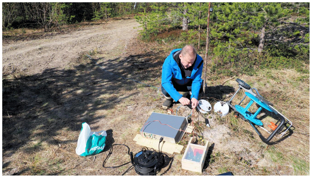
Figure 5. Pekka Korkeakangas tunes up the fixed loop (ca. 100 m by 100 m) electromagnetic transmitter in Ervastinranta in May 2021.
The system is powered by a basic 2-kilowatt generator. The box with a transparent plastic lid contains transmitter electronics. The large grey box in the middle is a power amplifier. Image published with the permission from Pekka Korkeakangas.
Figure 6 shows the small portable EM transmitter. It consists of an insulated wire wrapped around a plywood frame that is held together with two aluminum rods. The electronics of the transmitter are located inside the plastic “lunch box” in the middle of the loop. As in case of the fixed loop transmitter, the electronics consist of a microcontroller, signal generator, GNSS unit, and SD card for data storage. The transmitter is powered by a LiPo battery providing a current of about 1 A to the loop. The diameter of the loop is 1.04 meter and the number of wire-turns around the loop is N= 13. Thus, the dipole moment of the small transmitter is about 11 Am2. The small GNSS antenna can be seen at top of the electronics box. Pekka Korkeakangas is seen in the background with the EM receiver unit. The measuring tape on the right is used to keep the Tx-Rx distance the same when the system is moved along the road. The mass of the transmitter unit is about 1.2 kg without the battery and about 1.7 kg with 6-cell 12V LiPo battery. Because of its low weight the transmitter suite UAV based surveying.
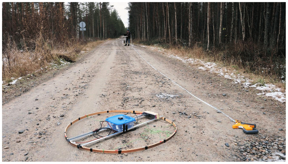
Figure 6. The small portable electromagnetic transmitter loop used in Lintumaansuo field tests in October 2020.
Transmitter electronics are inside the plastic ‘lunch box’. The diameter of the loop is about 1 m and it contains 13 loop windings giving a dipole moment of about 11 Am2.
In the current version of the small EM loop transmitter (Figure 6), there is no IMU (inertial measurement unit) that would provide orientation (e.g., roll, pitch and yaw angles) of the loop. Moreover, the recording of current and position is made at the frequency of 1 Hz, which is a bit too low for a transmitter to be carried and flown by a drone. These settings, however, can be changed by modifying the software running the microcontroller and will be implemented in the next prototype of the small EM transmitter.
In the present versions (Louhi prototype 3) of both transmitters, only one frequency of about 9 kHz is used. This limitation is due to system testing that has taken more time than expected. Now that the tests have shown that the system, especially the receiver, is working properly at the selected frequency, more frequencies can be added safely. The next version of the Louhi EM system will operate at three frequencies simultaneously. The tuning of the transmitter for minimum impedance is not as efficient anymore, but it is a small price to pay for the increase in the information content of the EM system due to wider frequency range and, consequently, wider range of depth of exploration.
Louhi EM receiver
The light-weight three-component EM receiver is the key part of the Louhi EM measurement system. The same receiver unit is used with both the fixed loop transmitter as well as the small moving transmitter loop.
Figure 7 shows the third prototype of the EM receiver used in Lintumaansuo field tests in October 2020. The three-component receiver loop consists of three rectangles that are perpendicular to each other so that they form an octahedron. The distance between opposite vertices of the octahedra is about 1 meter. The box in the middle contains the electronics of the receiver unit. The receiver, which is based on an Arduino Due (AD) microcontroller, comprises pre-amplifiers for the three loops, AD converters, a GNSS unit for time and location, IMU for orientation information, and a SD card for data storage. The receiver can be connected to a PC laptop for real-time data analysis and setup. With a click of a switch the receiver operates as a stand-alone device that stores the data onto an SD card to be collected via USB interface. The third prototype uses two GNSS antennas which are seen on top of the box. One is used for the timing only and the other is used by the IMU to determine the position and orientation. The mass of the receiver unit is about 1.4 kg without the battery and about 1.9 kg with a 6-cell 12 V battery. Because of its low weight the receiver suits UAV based surveying.
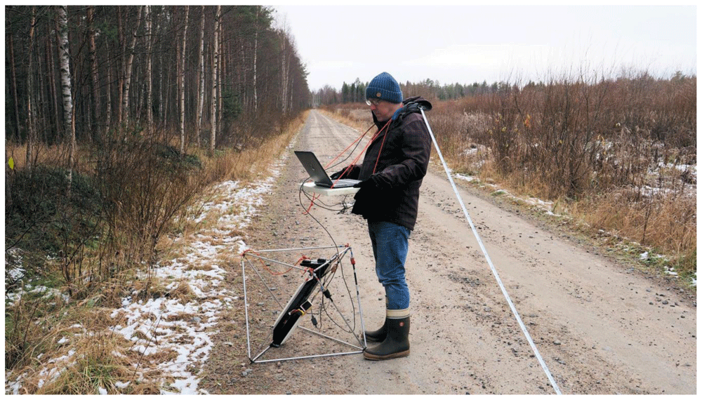
Figure 7. Louhi electromagnetic receiver used in a moving loop measurement in Lintumaansuo in October 2020.
The receiver consists of three rectangles that are perpendicular to each other so that they form an octahedron. The box in the middle contains Global Navigation Satellite System (GNSS) units, orientation sensors and receiver electronics with pre-amplifiers. The receiver can be connected to a PC laptop for real-time data analysis but it also works as a stand-alone instrument. Image published with the permission from Pekka Korkeakangas.
Louhi EM receiver is built around an embedded microcontroller (Arduino Due). The microcontroller digitizes (12-bit analog-to-digital converter, ADC) the analog signals coming from the receiver loops and uses the GNSS signal for accurate time synchronization of the three components. Instead of measuring a high-frequency time-series and computing the in-phase and quadrature components in post-processing, Louhi receiver performs signal stacking and processing using its embedded software. Presently, the Louhi data are measured once per second, but the sampling rate can be increased to enable better spatial sampling when the receiver is being towed by a drone at the speed of about 10-15 m/s.
Figure 8 shows Pekka Korkeakangas operating the Louhi operation software. This dedicated PC software, written in Python programming language, is used to modify the settings of the EM receiver, perform receiver calibration, and to visualize and analyse the measured three-component data in real-time (see Software availability). Data can be stored to PC hard disk and old data can be read in for closer analysis. When the receiver is used as a stand-alone device, the operation software is used to read the data from the SD card and to perform the required data post-processing steps.
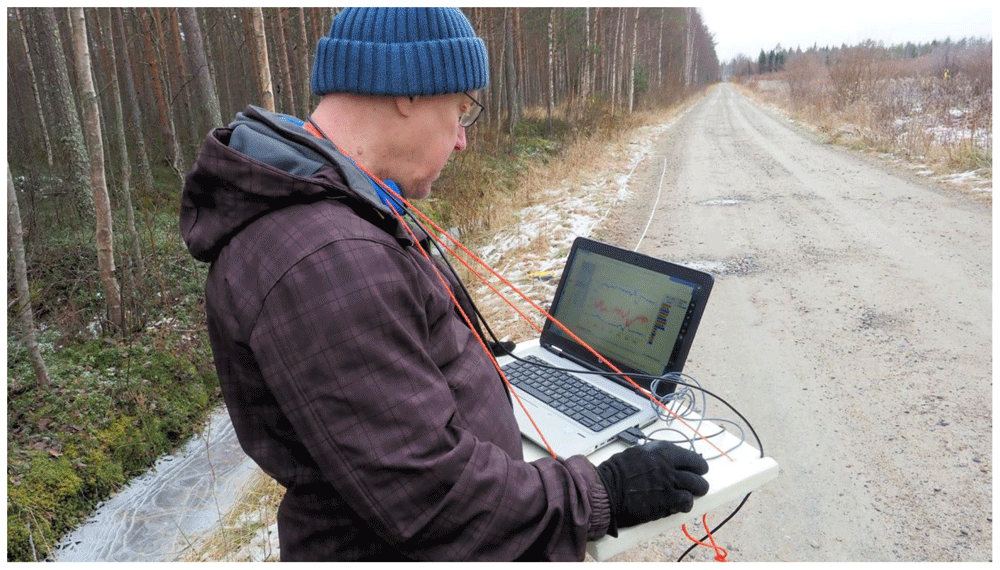
Figure 8. The dedicated PC software used for real-time analysis of the receiver data and to set the measurement parameters is an integral part of the Louhi electromagnetic (EM) survey system.
Image published with the permission from Pekka Korkeakangas.
Receiver calibration is perhaps the most important part of successful EM measurements. The calibration ensures that the amplitude and phase of the signals coming from each of the three coils/loops are timed and scaled so that the rotation of the field components yields correct values. The calibration also checks the orthogonality of the three receiver loops. Without calibration the amplitude and phase of one of the channels (XYZ) will differ from each other. The gain and calibration correction are made by the PC operation software either in real-time or when the data are read from the receiver memory. The PC software is important for system development. It provides means to quickly see the effect of various digital signal processing algorithms as the microcontroller of the receiver unit does not have strength for heavy computational tasks of data processing. Consequently, the PC operation software is constantly under development too.
Louhi EM response
Presently, the EM data recorded by the EM receiver unit is not calibrated in a known EM source field. Thus, the recorded data cannot be transformed into true values of the magnetic field (nT or pT) or its time derivative (nT/s or pT/s). However, the orthogonality of the three receiver loops and their mutual interaction is taken into account by making receiver calibration before the measurements. Receiver calibration is also needed whenever the receiver experiences a sudden impact that might change its physical properties and shape.
Presently, the Louhi EM response is simply the device response of the three channels. The response is gain corrected and scaled based on receiver calibration, and rotated to the world coordinates as NED components. GNSS time is used to provide in-phase and quadrature components of the EM response. At the moment, the Bz/Br-ratio is used for data interpretation because knowledge on the primary field is not available. In the future, the operation software will synchronize the data (current) measured by the transmitter unit with the receiver data. This enables computation of the primary (free-space) magnetic field (B0) at the receiver location and to provide normalized response components (Bx/B0, By/B0 and Bz/B0) that are commonly used for moving loop EM data (e.g., Frischknecht et al., 1991).
UAV platforms
Originally, Radai had purchased a vertical take-off and landing (VTOL) drone (Great Shark) for radiometric gamma measurements in 2020 from a Chinese company Foxtech. The drone was modified for EM measurements and given the name Mother-Goose. Unfortunately, the wingspan of Mother-Goose exceeds 3 meters, and hence, falls into a stricter category of drone operations according to EU drone legislation. Therefore, Radai plans to purchase and deploy a slightly smaller VTOL drone (Baby-Shark/Goose) with a wingspan of 2.5 m in the EM surveys in the future. Technical parameters of the Goose and Mother-Goose VTOL drones are presented in Table 1.
Table 1. Parameters of Goose and Mother-Goose vertical take-off and landing (VTOL) drones.
| Parameter | Goose | Mother-Goose |
|---|
| Wingspan | 2.5 m | 3.2 m |
| Length | 1.4 m | 1.75 m |
Ready-to-fly
weight | 5.6 kg | 9 kg |
| Payload | < 7.4 kg | < 12 kg |
| Speed | 16-30 m/s | 18-32 m/s |
| Endurance | Max 2.5 h | Max 3 h |
Figure 9 shows Mother-Goose vertical take-off and landing (VTOL) drone used to carry the Louhi electromagnetic transmitter and receiver units, and Figure 10 shows the Mother-Goose VTOL drone carrying the Louhi EM receiver and transmitter units during the first flight tests in Pateniemi in Oulu in June 2021. The purpose of the flight test was to demonstrate that the Mother-Goose drone is capable of lifting the EM equipment and making flight operations safely. The experiences Radai has obtained from similar drones used in magnetic surveying during the last year have demonstrated that VTOL drones are highly efficient and suit geophysical surveying well.
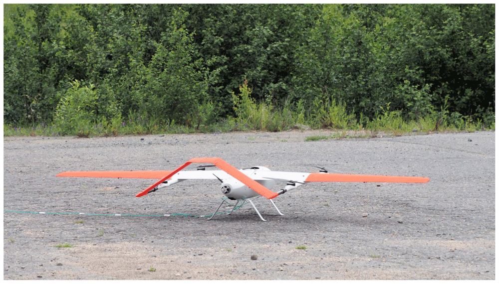
Figure 9. Mother-Goose vertical take-off and landing (VTOL) drone used to carry the Louhi electromagnetic transmitter and receiver units in Pateniemi.
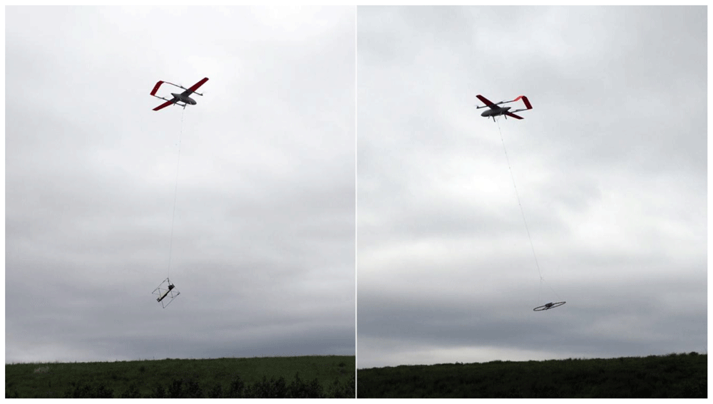
Figure 10. Mother-Goose vertical take-off and landing (VTOL) drone carrying the Louhi electromagnetic receiver (left) and transmitter (right) in Pateniemi.
Use case
Lintumaansuo
Lintumaansuo test site is located in Kiiminki about 20 km north of Oulu, Finland. The site is characterized by a SE-NW directed and almost vertical zone of black schists (pyrrhotite) that create both an electromagnetic conductivity anomaly and magnetic susceptibility anomaly (Honkamo, 1988). Along the Lintumaansuontie road, where the Louhi EM tests took place, the magnetic anomaly shows two closely the located magnetized bodies. Previous VLF measurements (Mursu, 1991), however, do not identify separate conductors.
In October 2020, Radai made the first field tests with the Louhi prototype 3 receiver system in Lintumaansuo using both the small (diameter 1 m) moving loop system and large (120 m by 120 m) fixed loop system. Figure 11 shows the location of the data points from both measurements and the location of the large fixed loop. The separation between the small loop transmitter and receiver was about 25 m. The original data associated with the survey as well as some extra information like digital maps and terrain models are available in Underlying data (Pirttijärvi et al., 2021).
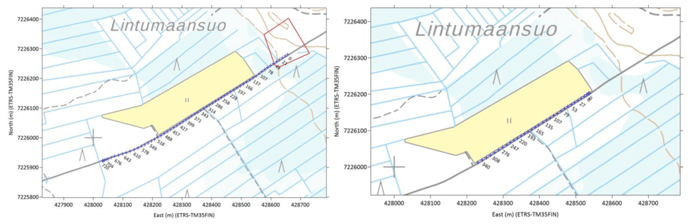
Figure 11. The location of the loop (red polygon) data points from a fixed loop measurement (left) and the location of the data points from a moving small loop measurement (right).
The labels depict the distance from the beginning of the profile. Background map © National Land Survey of Finland, 2020.
The orientation corrected sensor data (Bu=Bz,Bn=Bx,Be=By) and the Bz/Br-ratio from the small loop measurement are shown in Figure 12. The radial component (Br) is the horizontal field component directed away from the center of the loop and Bz is the vertical component. The Bz/Br-ratio is shown both as the real and imaginary component and as the amplitude and phase (atan(Bz/Br)). Bearing in mind that the up component (Bu) of the small loop measurement corresponds to HLEM (horizontal loop EM) response or Slingram response, the negative peak anomaly at location X=170 m clearly shows the NE location of the conductor. The weaker minima at location X= 210 m corresponds either to the second conductor or the SW side of a thick conductor.
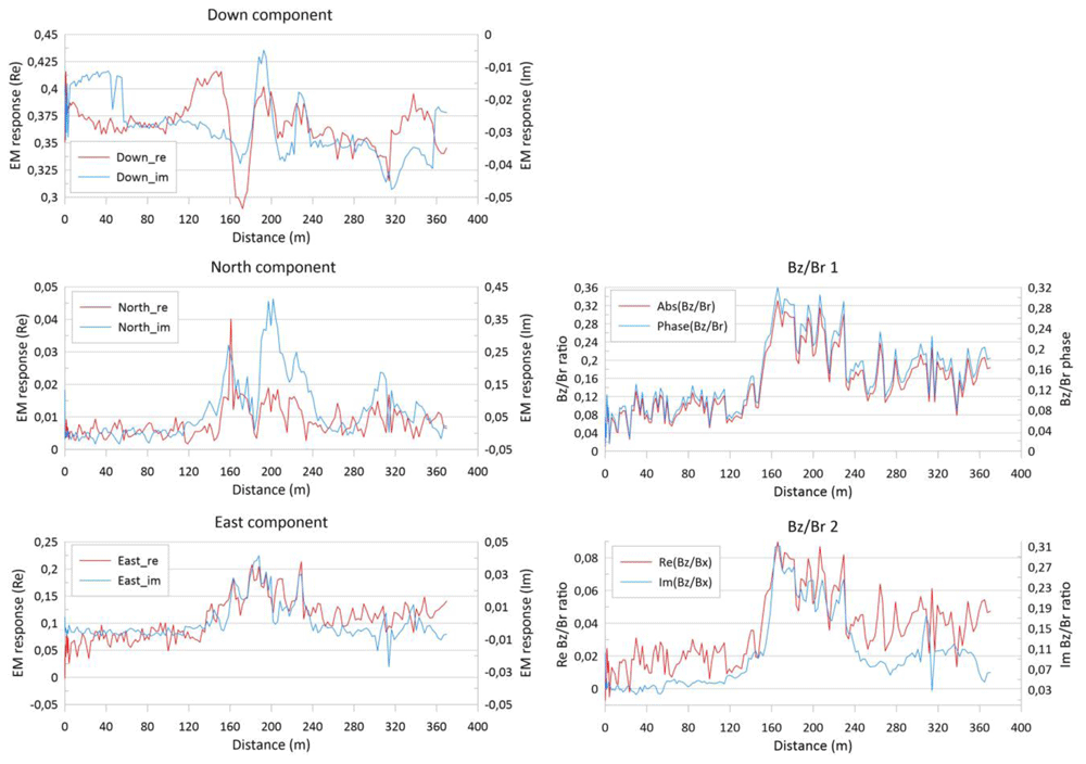
Figure 12. Louhi electromagnetic data plotted as the in-phase (real) and quadrature (imaginary) parts of down, north and east components (left) and as the amplitude and phase (radians) and real and imaginary parts of the Bz/Br-ratio (right) from the survey with small moving loop data from Lintumaansuo.
Bz/Br is the ratio between the vertical component (Bz) and the radial component (Br) of the measured response.
The data were interpreted using 1D inversion by the Lempo1D software that was also being developed in the NEXT project. Lempo1D is based on the AEMinv software (Pirttijärvi, 2014). It uses linearized inversion with lateral constraining to find the conductivity and thickness of layered 1D earth model such that the fit between the measured data and modelled response is minimized. Lempo1D is private software used for Radai’s in-house development work and is not publicly available. Em1dinv (Auken et al., 2005) and is successor Aarhusinv (Auken et al., 2014), are similar open source software that could be used for the data interpretation.
The results from the Lempo1D inversion and the fit between the measured data and modelled response are shown in Figure 13 and Figure 14 for the small loop and fixed loop system, respectively. Because of the short loop separation, the small loop data was interpreted using a single layer model. Thus, the pseudo-section in Figure 13 is essentially the same as apparent resistivity. The fixed loop data was interpreted using a two-layer model. Because only a single frequency was used the accuracy of interpreted layer thickness is ambiguous.
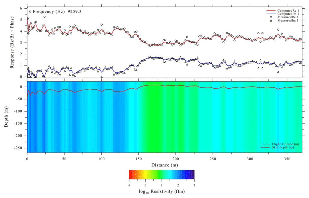
Figure 13. Lempo1D interpretation of small moving loop data from Lintumaansuo.
The graph on the top shows the fit between measured data (symbols) and modelled response (solid lines). The graph on the bottom depicts a resistivity pseudo-section along the profile.
Despite the high noise level due to inaccurate real-time orientation correction, both datasets were successfully interpreted with Lempo1D software and the pseudo-sections illustrating the conductivity/resistivity along the profiles are geologically meaningful. The same 100 m wide conductive zone is seen both between 150–250 m in moving loop data and 300–400 m in fixed loop data. Moreover, the resistivity of the host medium is different on opposite sides of the conductive zone. Because of a better depth extent, the fixed loop data resolves two different conductors. The interpreted resistivity values at the beginning of the fixed loop profile (Figure 14) are overestimated because the receiver is so close to the loop. The spiking effect of the loop is clearly seen in the modelled response at location X= 50 m.
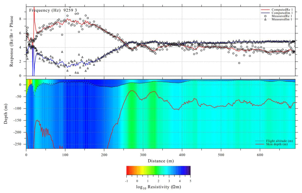
Figure 14. Lempo1D interpretation of fixed loop data from Lintumaansuo.
Ervastinranta
Ervastinranta test site is located in Haukipudas about 20 km north of Oulu, Finland. The site is characterized by an EW directed contact between conductive (20 Ωm) sandstones of Muhos formation in south and resistive mica schists of Kiiminki formation (Honkamo, 1988). According to previous studies made as a part of geophysical field courses of the University of Oulus, the contact is almost vertical, and the thickness of the sandstones is ca 100 m close to the contact.
In May 2020, Radai made the field tests with the Louhi prototype 3 receiver system in Ervastinranta using a large (100 m by 100 m) fixed loop system. Figure 15 shows the location of the data points from two measurements and the location of the large fixed loop. In this case, the data were transformed into the amplitude of the Br/Bz ratio. Both measurements were made at the same location. Profile #1 was measured using a stop-and-go method, where the receiver was carried by hand from point to point and kept immobile at ground level for about 10 seconds at each measurement site. Although no averaging was made on stop-and-go data, it gives good quality data at each measurement point. Profile #2 was measured using an on-the-fly method, where the EM receiver was manually carried at the height of about 0.5 m above the ground. As profile #2 was measured without any pauses, it gives data that resembles airborne surveying, although the receiver will sway less when it is carried by a drone than when it is carried while walking. The original data associated with the survey as well as some extra information like digital maps and terrain models are available in Underlying data (Pirttijärvi et al., 2021).
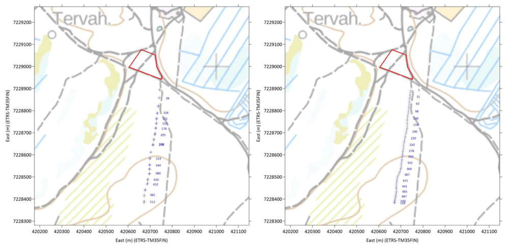
Figure 15. The location of the fixed loop electromagnetic (EM) transmitter (red polygon) and the location EM data points of profiles #1 (left) and #2 (right).
The blue labels depict the distance from the beginning of the profiles. Background map © National Land Survey of Finland, 2020.
Like the Louhi EM data from Lintumaansuo (Figure 11–Figure 14), the data from Ervastinranta were interpreted using 1D inversion by the Lempo1D software. The Aarhusinv software (Auken et al., 2014) could have been used for data interpretation as well. The results from the inversion and the fit between the measured data and modelled response are shown in Figure 16 and Figure 17 for profiles #1 and #2, respectively. As in case of Lintumaansuo (Figure 14) both datasets were interpreted using a two-layer model, where the top layer models soil overburden and bottom layer models the basement rocks. Because only a single frequency was used, the accuracy of interpreted layer thickness is ambiguous. Comparison of the data of Figure 16 and Figure 17, shows that the stop-and-go data (Profile #1, Figure 16) is less noisy and data are clustered around their “true” value. According to the test, the fixed loop of size 100 m by 100 m provides fairly good quality data up to the distance of about 500 m away from the loop.
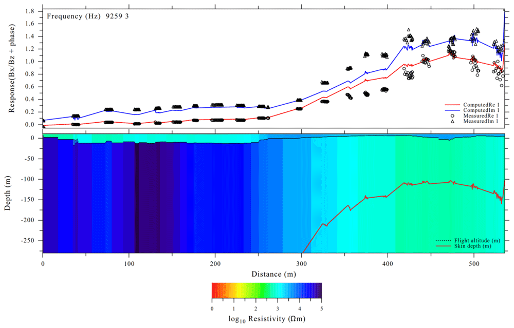
Figure 16. Lempo1D interpretation of fixed loop data from Ervastinranta profile #1 (stop-and-go).
All in all, both inversions produce similar results. Despite the higher noise level of profile #2 (on-the-fly, Figure 17), the interpreted model is very similar to that from profile #1 (stop-and-go). In both inversions, the contact between resistive Kiiminki mica schists (north) and conductive Muhos sandstones (south) is seen at location X= 320-350 m. Based on the tests, the Louhi EM systems suits geological mapping.
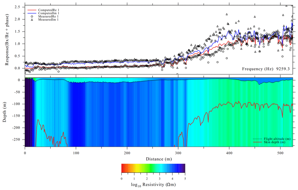
Figure 17. Lempo1D interpretation of fixed loop data from Ervastinranta profile #2 (on-the-fly).
Conclusions
Radai Ltd developed a new drone-based geophysical electromagnetic (EM) survey system (Louhi) in the EU funded Horizon 2020 project NEXT – New Exploration Technologies. The development work of the Louhi system has taken more time than expected. The third prototype of Louhi has two operation options, the first uses a fixed ground loop as an EM source and the second uses a small portable loop EM transmitter. Both systems use the same 3-component EM receiver which is so light that it can be carried by a drone. Since it is not useful to make many tests with an unfinished system that is soon to be replaced with a better one, only a few field tests have been made with the third prototype of the Louhi system. However, the field tests made so far clearly demonstrate that both fixed loop system and moving loop system do provide geologically meaningful data. Moreover, the flight tests have shown that both the small transmitter and the receiver can be carried by a drone, and that the flight operations can be made safely. The development work continues in the new H2020 GoldenEye project and the first airborne field surveys with the new multi-frequency version of the Louhi EM system will be made in 2022.
Data availability
Underlying data
Zenodo: Louhi EM test data. http://doi.org/10.5281/zenodo.5082559 (Pirttijärvi et al., 2021).
This project contains the following underling data:
Louhi_EM-test-data.zip (zip-compressed collection of files containing the data associated with Lintumaansuo and Ervastinranta field tests in Figs 11-17. The data include both raw and processed data and background data such as terrain models, maps and loop coordinates. The data are stored as column formatted text files, and hence, can be used with any other software. Maps are stored as PNG images with PGW geotagging information (ESRI world file). DEM data are stored in ESRI Ascii grid format, that are compatible with most GIS (geographical information system) software, such as the open source QGIS).
Readme_Louhi_EM-test-data.txt (general text file describing the contents of the zip file).
Data are available under the terms of the Creative Commons Attribution 4.0 International license (CC-BY 4.0).
Software availability
The PC operation software of Louhi system is an integral part of the Louhi device. Due to prospects for commercial exploitation the PC operation software is not publicly available at the moment. For particular availability in case of co-operative projects, please contact the corresponding author (markku.pirttijarvi@radai.fi).
Ethics and consent
Ethical approval and consent were not required.