Development and validation of an open-source CFD model for the efficiency assessment of data centers

Aras Dogan; Sibel Yilmaz; Mustafa Kuzay; Ender Demirel

doi:10.12688/openreseurope.14579.1

Development and validation of an open-source CFD model for the efficiency assessment of data centers

Article

Authors & roles Authors

Peer review record Peer review

Metrics

Cite

Section

Method Article

Published

March 24, 2022

DOI

https://doi.org/10.12688/openreseurope.14579.1

Versions

March 24, 2022 (Published Manuscript Under Review 1.0)

European Commission

Grant ID(s): 956059

Views

362

Downloads

Citations

See full metrics

Data center, cooling efficiency, thermal structure, efficiency assessment, CFD, OpenFOAM

Abstract

In this study, an open-source computational fluid dynamics (CFD) model was developed based on OpenFOAM libraries for the accurate and robust simulation of thermal distribution in a data center. Two boundary conditions were developed for the temperature field in the black-box modeling of server components. The numerical model was first validated by comparing numerical results with the experimental measurements for three benchmark problems in the field of thermal engineering. Then, thermal distribution in an open-aisle data center was simulated using the proposed numerical model and results were compared with the experimental measurements. The consistency between numerical results and previous experimental measurements indicates that the present numerical model can be reliably used for the efficiency assessment of air-cooled data centers. Efficiency of the data center can be evaluated with respect to four metrics in the proposed numerical model. In addition to the determination of the overall efficiency, distribution of the efficiency can be monitored over the racks to capture thermal zones where the efficiency decreases due to the recirculation effects and cold air by-pass.

Corresponding author

Ender Demirel

0000-0002-0440-7866

edemirel@dstechno.net

Grant information

This research was financially supported by the European Union’s Horizon 2020 research and innovation programme under the grant agreement No 956059(Artificial-Intelligence-Augmented Cooling System for Small Data Centres [ECO-Qube]).

The funders had no role in study design, data collection and analysis, decision to publish, or preparation of the manuscript.

This work is licensed under a Creative Commons Attribution 4.0 International License.

First version published

March 24, 2022 (https://doi.org/10.12688/openreseurope.14579.1)

Latest version published

March 24, 2022 (https://doi.org/10.12688/openreseurope.14579.1)

Plain language summary

Efficiency assessment of an existing data center is important for its energy considerations. This study presents an open-source tool for the assessment of thermal and cooling efficiencies based on computational fluid dynamics (CFD) simulations. The efficiency of a data center can be evaluated according to the efficiency metrics in a consistent manner. The proposed tool determines not only the overall efficiency of the data center according to four metrics, but also the variations of the efficiency indexes over the racks, which is fundamental to the development of the zonal cooling concept as a holistic approach in data centers. This innovative approach in the CFD simulations of data center enables to capture server components, where thermal efficiency decreases due to the hot air recirculation and cold air by-pass.

Symbol list

ρ Density (kg m^-3)

u_i Mean velocity in the i-direction (m s^-1)

p Pressure (kg m^-1 s^-2)

μ Dynamic viscosity (kg m^-1 s^-1)

μ_t Turbulent viscosity (kg m^-1 s^-1)

g_i Gravitational acceleration in the i-direction (m s^-2)

h Enthalpy (m² s^-2)

S_i Momentum source in the i-direction (m s^-1)

k Turbulence kinetic energy (m² s^-2)

ω Specific turbulence dissipation rate (s^-1)

D Darcy coefficient (m^-2)

F Forchheimer coefficient (m^-1)

Ф Porosity

T Temperature (̊C)

ΔT Temperature jump (̊C)

$\dot{m}$ Mass flux (kg s^-1)

C_p Specific heat capacity (J kg^-1 K^-1)

P Power consumption (W)

Q Flow rate (m³ s^-1)

Introduction

Data centers are becoming energy intensive infrastructures with the rapid developments in fifth generation (5G) communication, artificial intelligence (AI) and simulation technologies in high performance computing (HPC) clusters. Data centers have experienced a drastic increase in workloads due to the digitization of social and professional practices during pandemic conditions. Cooling of information technology (IT) equipment has a substantial power demand since 40% of the total power consumption in data centers originates from the cooling devices¹.

Data centers are conventionally designed as enclosed environments for the reliable operations of the IT equipment, which are extremely expensive infrastructures. Most of the data centers facilitated in different climate zones have been cooled with air². A uniform airflow is required in ideal conditions from computer room air conditioning (CRAC) units to the IT equipment without mixing of the cooled air with the hot air exhausted from IT equipment, since recirculating hot air results in increasing air temperature beyond the limits suggested by the regulations². Moreover, cold air by-pass encountered in room data centers is another design challenge that may reduce cooling efficiency and increase power consumption by the CRAC units. Thus, a well-designed thermal environment should be created inside the data center to reduce power consumption by the cooling equipment.

Simulation of thermal structure inside a data center by using computational fluid dynamics (CFD) methods has become a thriving research area, with the rapid developments in numerical models and computational power in the last decade. Open-source CFD models are gaining importance in academic research because problem-specific features can be developed based on open-source libraries and incorporated into the computational model, to achieve an accurate and robust solution of the problem. Commercial software in the market are capable of simulating thermal flow inside a data center³. Cho et al.³ performed a series of numerical simulations for different design alternatives using a commercial software to evaluate thermal environment based on efficiency indexes. Nada and Said⁴ investigated the effect of CRAC layout on the thermal environment of high-density data centers using a commercial CFD software, and found that locating the CRAC unit perpendicular to the racks enhanced performance of the data center. However, open-source CFD models are not yet extensively used in data center applications and related works are rare in this area.

In this work, an open-source CFD model was developed based on OpenFOAM libraries, which can be freely accessed for the flow and thermal simulations of data centers and validated with the experimental measurements in the field of thermal engineering. The validated numerical model was employed to simulate thermal structure of an open-aisle data center and results are validated with the previously reported experimental measurements. Efficiency metrics can be calculated at each IT equipment and CRAC unit, which allows to detect thermal zones where the efficiency is low.

Methods

Numerical model

Compressible turbulent flow inside the data center can be represented by the following continuity, momentum and energy conservation equations including buoyancy effects:

\frac{\partial ρ}{\partial t} + \frac{\partial}{\partial x_{i}} (ρ u_{i}) = 0 (1)

\frac{\partial (ρ u_{i})}{\partial t} + \frac{\partial}{\partial x_{j}} (ρ u_{i} u_{j}) = - \frac{\partial p}{\partial x_{i}} + \frac{\partial}{\partial x_{j}} [(μ + μ_{t}) (\frac{\partial u_{i}}{\partial x_{j}} + \frac{\partial u_{j}}{\partial x_{i}})] + ρ g_{i} + S_{i} (2)

\frac{\partial (ρ h)}{\partial t} + \frac{\partial}{\partial x_{j}} (ρ u_{j} h) = \frac{\partial}{\partial x_{j}} [(μ + μ_{t}) \frac{\partial h}{\partial x_{i}}] (3)

Where ρ is the density of the fluid, u_i (i ∈ [1,2,3]) is the mean velocity component in the i-direction, t is the time, p is the mean pressure, x_i and x_j are the Cartesian coordinates, g_i is the gravitational acceleration in the i-direction, h is the Favre-averaged enthalpy, S_i is the momentum source, μ and μ_t are molecular and turbulent viscosities, respectively. Pressure is decomposed to hydrostatic and non-hydrostatic parts as p_d = p – ρg_ix_i in a buoyancy-driven flow. Here, the non-hydrostatic part is calculated by removing the hydrostatic part from the piezometric pressure p. Turbulent viscosity can be calculated from the following equation in the k – ω turbulence model to account for adverse pressure gradients and boundary layer effects near the walls: σ

ν_{t} = \frac{a_{1} k}{m a x (a_{1} ω, S F_{2})} (4)

Where, k and ω are calculated from the following transport equations:

\frac{\partial k}{\partial t} + u_{i} \frac{\partial k}{\partial x_{i}} = \frac{\partial}{\partial x_{i}} [(ν + σ_{k} ν_{t}) \frac{\partial k}{\partial x_{i}}] + P - β^{*} k ω (5)

\frac{\partial ω}{\partial t} + u_{i} \frac{\partial ω}{\partial x_{i}} = \frac{\partial}{\partial x_{i}} [(ν + σ_{ω} ν_{t}) \frac{\partial ω}{\partial x_{i}}] + α S^{2} - β ω^{2} + 2 (1 - F_{1}) \frac{σ_{ω 2}}{ω} \frac{\partial k}{\partial x_{i}} \frac{\partial ω}{\partial x_{i}} (6)

Coefficients that appear in the turbulence equations can be found in the literature⁵. Perforated plates and screens are widely used in data centers to achieve a uniform flow from CRAC units to the racks³. Moreover, energy losses occur through the servers due to the resistance by the electronic components embedded in the servers. Thus, the numerical model should be sensitive to the energy losses through the perforated plates and IT equipment. A source term is added to the momentum equations to represent resistance effects encountered in the porous zone. The Darcy-Forchheimer porosity model is the most common approach to model inertia and viscous resistance by the porous medium. The source term is calculated from the following equation:

S_{i} = - (ν D - \frac{1}{2} u_{j j} F) u_{j} (7)

Here, the Darcy and Forchheimer coefficients must be determined to represent the investigated porous media. The Darcy and Forchheimer coefficients can be calculated from the following empirical equations^6,7:

D = \frac{120 {(1 - Φ)}^{2}}{Φ^{3} R^{2}} (8)

F = \frac{2.3 (1 - Φ)}{Φ^{3} R} (9)

Here Ф is the porosity and R is the hydraulic radius, which can be calculated at the inlet of the server. Darcy and Forchheimer coefficients are calculated using the above expressions and defined in the fvOptions file of OpenFOAM in Figure 1 to calculate pressure drop along the porous zone.

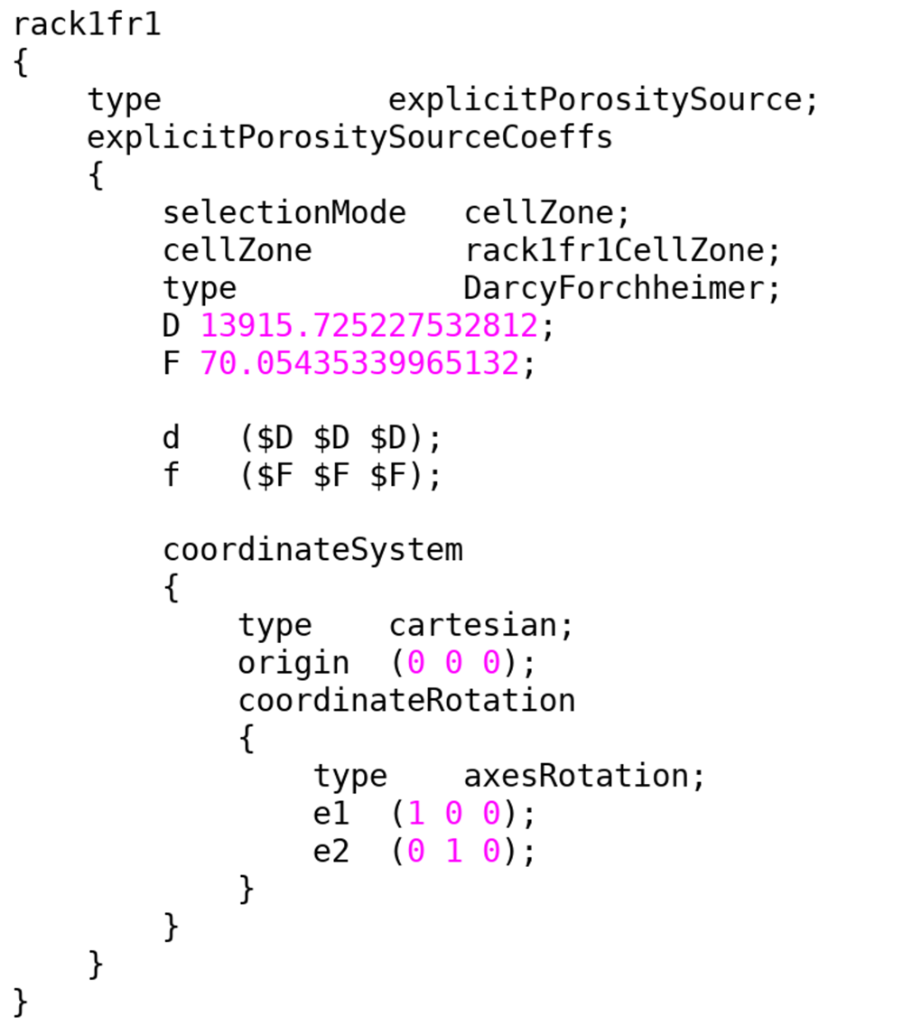
Figure 1. Definition of the Darcy-Forchheimer coefficients in the fvOptions file.

Efficiency metrics

Efficiency metrics are defined as non-dimensional numbers to evaluate the thermal and cooling performance of a data center. Several metrics have been proposed by the researchers for the assessment of the efficiency of a data center. The inlet temperature of an IT equipment is expected to be equal to the supply temperature from the CRAC in ideal conditions, in which hot and cold air are not mixed. The inlet temperature of an IT equipment is higher than the supply temperature from the CRAC, and the inlet temperature of the CRAC is lower than the exhaust temperature from the IT equipment in real conditions. The rack cooling index (RCI) compares intake temperature with the recommended and allowable temperatures to evaluate the cooling performance:

RC I_{H I} = [1 - \frac{\sum_{i = 0}^{n} (T_{i} - T_{m a x - r e c})}{n \times (T_{m a x - a l l} - T_{m a x - r e c})}] \times 100 % (10)

RC I_{L O} = 1 - [\frac{\sum_{i = 0}^{n} (T_{m i n - r e c} - T_{i})}{n \times (T_{m i n - r e c} - T_{m i n - a l l})}] \times 100 % (11)

Where T_max–rec and T_min–rec are the recommended maximum and minimum temperatures, T_max–all and T_min–all are the allowable maximum and minimum temperatures, respectively. Allowable and recommended maximum and minimum temperatures² are given in Table 1.

Table 1. Allowable and recommended temperatures².

T_max-rec [°C]	T_min-rec [°C]	T_max-all [°C]	T_min-all [°C]
27	18	32	15

It should be considered that the RCI_HI captures only the IT equipment where the inlet temperature is greater than the maximum recommended temperature, and the RCI_LO captures the IT equipment where the inlet temperature is lower than the minimum recommended temperature. As given in Table 2, the cooling efficiency of a data center can be classified as ideal, good, acceptable and poor according to the calculated RCI value.

Table 2. Rating of the RCI⁸.

Rating	RCI
Ideal	100%
Good	≥ 96%
Acceptable	91 – 95%
Poor	≤ 90%

The performance of the CRAC unit can be evaluated in terms of cold air by-pass or hot air recirculation according to the return temperature index (RTI):

R T I = [1 - \frac{T_{R e t u r n} - T_{S u p p l y}}{Δ T_{e q u i p}}] \times 100 % (12)

Where ΔT_equip is the average temperature rise of the IT equipment, T_Return and T_Supply are the mean temperatures at the inlet and outlet of the CRAC unit, respectively. The average temperature rise can be calculated from the following equation:

Δ T_{e q u i p} = \frac{\sum_{i = 0}^{n_{I T}} [{(T_{o u t})}_{i} - {(T_{i n})}_{i}] {\dot{m}}_{i}}{\sum_{i = 0}^{n_{I T}} {\dot{m}}_{i}} (13)

Where, n_IT is the number of IT equipment and $\dot{m}$ _i is the calculated mass flux through the IT equipment. Hot air recirculation occurs when the RTI is higher than 100% and cold air by-pass occurs when the RTI is lower than 100%. Thus, deviations from 100% exhibit a low thermal efficiency in a data center. Thermal efficiency of the data center can be evaluated according to the RTI value in Table 3:

Table 3. Rating of the RTI⁸.

Rating	RTI
Target	100%
Recirculation	> 100%
By-pass	< 100%

The Supply Heat Index (SHI) and Return Heat Index (RHI) introduced by Sharma et al.⁹ are dimensionless indicators to evaluate thermal performance of a data center:

S H I = \frac{δ Q}{Q + δ Q} (14)

Where Q and δQ are the total heat dissipation and the rise in enhaltpy of the air, respectively.

Q = \sum_{j} \sum_{i} {\dot{m}}_{i, j}^{r} C_{p} [{(T_{o u t}^{r})}_{i, j} - {(T_{i n}^{r})}_{i, j}] (15)

δ Q = \sum_{j} \sum_{i} {\dot{m}}_{i, j}^{r} C_{p} [{(T_{i n}^{r})}_{i, j} - T_{r e f}] (16)

Where, T_ref represents the vent tile inlet temperature, which is assumed to be equal to the supply temperature of the CRAC. The RHI represents the following total heat dissipation:

Q = {\sum_{k} \dot{M}}_{k} C_{p} [{(T_{i n}^{c})}_{k} - T_{r e f}] (17)

Where $\dot{M}$ _k and ${(T_{i n}^{c})}_{k}$ are the mass flux and inlet temperature of the k^th CRAC unit, respectively. Thus, the RHI can be calculated as:

R H I = \frac{Q}{Q + δ Q} = \frac{\sum_{k} {\dot{M}}_{k} C_{p} [{(T_{i n}^{c})}_{k} - T_{r e f}]}{\sum_{j} \sum_{i} {\dot{m}}_{i, j}^{r} C_{p} [{(T_{o u t}^{r})}_{i, j} - {(T_{r e f}^{r})}_{i, j}]} (18)

Use of open-source code enabled us to incorporate calculations of the efficiency metrics into the present open-source libraries and to assess the performance of a data center. Each metric was incorporated into the present open-source code as a function object to calculate metrics as a field inside the domain. This feature of the present numerical model enables us to capture thermal zones where thermal and cooling efficiencies decrease due to the recirculating flows and cold air by-pass. Snipped code of the function object for the RCI is given in Figure 2.

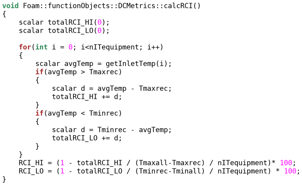
Figure 2. Snipped code for the calculation of the RCI as an object function.

The computational mesh of a typical data centre consists of a large number of computational cells to capture spatial and temporal variations in flow and thermal variables accurately. A huge memory is required to store coefficients of the linear system since sizes of the owner, and neighbour and diagonal matrices of each variable are proportional to the number of computational cells and faces. Thus, numerical simulations need to be performed with parallel computing on HPC clusters to achieve high-resolution numerical solutions in an acceptable duration. The computational domain was decomposed to sub-regions in parallel computing and each sub region was solved on a separate processor with the communication of each processor on a master processor using message passing interface (MPI). Sub-domains were connected to each other by processor boundaries to transfer calculated coefficients between sub-domains.

Modeling IT equipment

IT equipment can be modeled using open-box or black-box approaches in the CFD modeling of data centers. Mesh is created inside the server to solve airflow through a server and to apply a heat source in the open-box model. On the other hand, flow inside the server is not solved and a jump condition is applied for the temperature rise from the inlet to the outlet in the black-box approach. Specification of the flow rate through a server is challenging in the CFD modelling of an IT equipment. The most common approach is to fix the flow rate of the server according to the following empirical equation¹⁰:

Q = 212 \times P [m^{3} / h] (19)

This approach assumes that the flow rate is proportional to the power consumption of the server and independent of the pressure difference between hot and cold aisles. It should be noted that this approximation is applicable when server fans are controlled by the system and not by the user. The temperature rise can be calculated from the following equation in the black-box approach:

Δ T = \frac{P}{\dot{m} C_{p}} (20)

Here, the temperature rise ΔT is the function of the power consumption P and mass flux $\dot{m}$ through the server.

A zero gradient boundary condition was used for the temperature at the inlet and a jump boundary condition was used at the outlet to apply temperature rise according to the power consumption by the server. Special attention should be paid to the definition of the boundary conditions for the temperature field in the black-box model. It is assumed that the total power consumed by the IT equipment is converted to heat, and the generated heat is transferred to the air passing through the server. Thus, the temperature profile along the server changes due to the mixing effects induced by internal components of the IT equipment. As described in Figure 3, two boundary conditions were developed for the black-box model and incorporated into the numerical model to adjust outlet temperature depending on the inlet temperature field and calculated temperature rise.

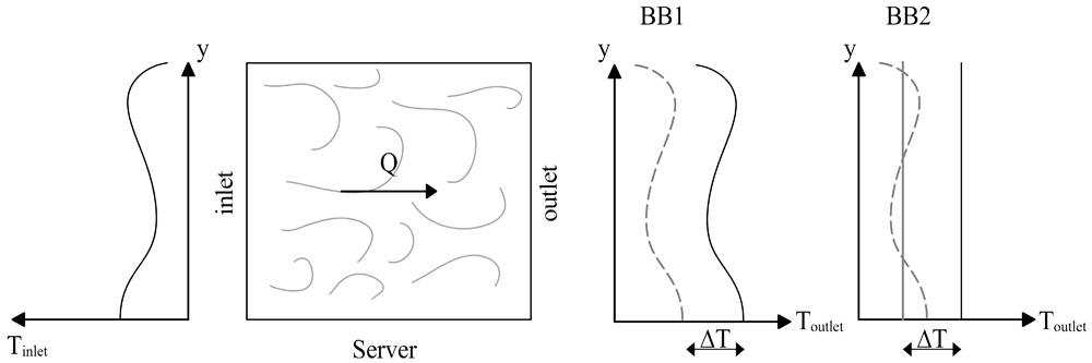
Figure 3. Temperature boundary conditions for the black-box model.

Inlet temperature profile was imposed at the outlet with an increment of ΔT in the black-box 1 (BB1) boundary condition:

T_{o u t l e t} (y) = T_{i n l e t} (y) + Δ T (21)

On the other hand, average temperature was calculated at the inlet and imposed at the outlet adding ΔT in the black-box 2 (BB2) boundary condition:

T_{o u t l e t} = \frac{T_{i} {\dot{m}}_{i}}{{\dot{M}}_{i n l e t}} + Δ T (22)

The BB1 and BB2 boundary conditions can be used to model an IT server. BB1 is preferred to use in the rack level modeling of data centers. Considering the mixing of the flow inside an IT equipment due to the internal components, BB2 is more appropriate than BB1 in the black-box modeling of an individual IT equipment.

Figure 4 shows the snipped code of the BB1 including mapping procedure between processors for parallel computing. The inlet and outlet boundaries can be located at the front and back covers of IT equipment. However, inlet and outlet boundaries were moved to internal domain of the servers in the present study to allow the flow to develop through the servers, to reduce stability issues originating from local changes in the computional domain.

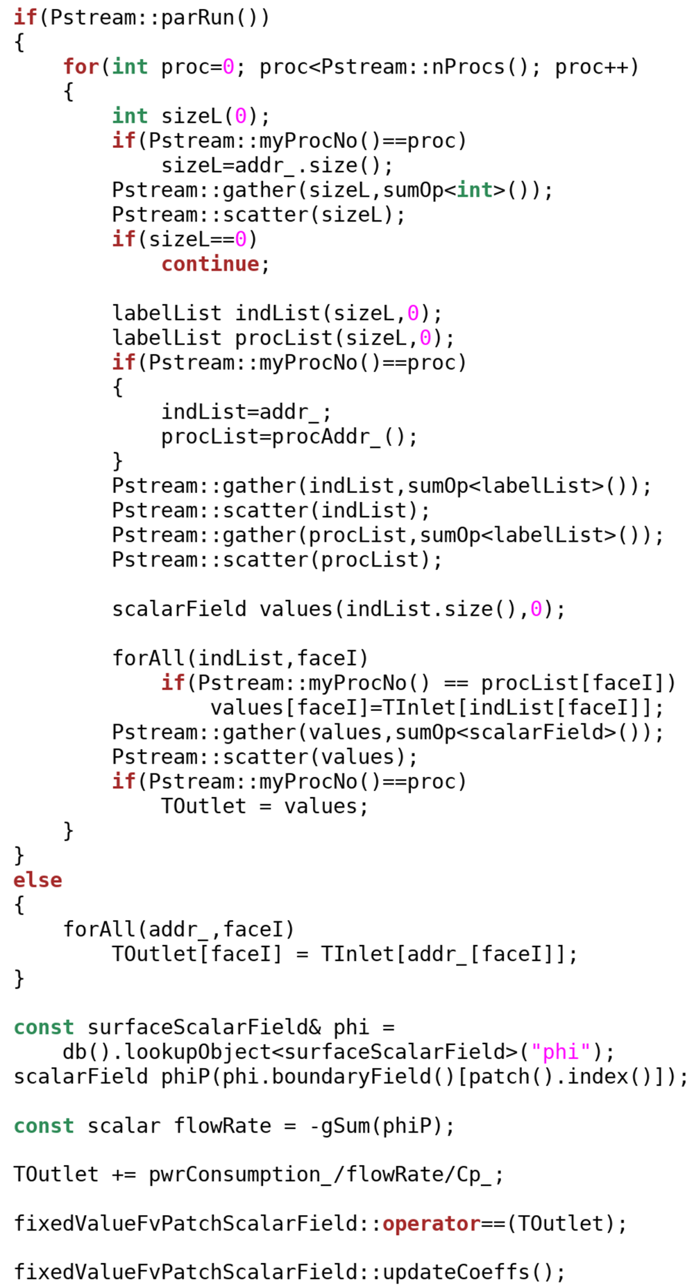
Figure 4. Snipped code for the BB1.

Boundary conditions were not defined in an open-box model, which made it more stable than black-box approach. A heat source was given to a cell zone inside the IT equipment and the temperature rise was calculated by the solver. The momentum source is defined as a fixed velocity inside the cell zone that covers the cross section of the IT equipment. Heat and momentum sources were given to the same cell zone which occupies the entire volume of the IT equipment.

Inactive IT equipment might be modeled as solid objects based on the assumptions of no heat source and airflow through the server. The first assumption can be justified such that heat is not generated when the IT equipment consumes no power. However, the latter assumption may not represent correct physical conditions since pressure differences between inlet and outlet boundaries may result in airflow through an inactive server. Thus, inactive servers should be modeled as porous regions in which energy loss and a pressure drop occur, even if the flow rate is small in comparison to that in active servers. Resistance by the micro-components to the flow passing through the IT equipment should be modeled while simulating airflow through the server. The best option is to use a porous medium approach inside an IT equipment, since microscopic modeling of each electronic component in the server will greatly increase the required computational memory and simulation duration. Moreover, inactive IT components should be modeled as porous zones instead of modeling as solid structures to allow airflow inside the server depending on the pressure difference between inlet and outlet. Porosity of the server can be set to a value between 0.35 and 0.65 for an IT equipment⁶.

Modeling CRAC units

In this study, CRAC units were modeled using the black-box approach, where a zero-gradient boundary condition was applied at the inlet and a fixed value was imposed at the outlet for the temperature. A fixed velocity was applied at the outlet to impose the flow rate of the CRAC unit, which can be obtained from the specification data sheet of an air-conditioning unit. Special attention is required for the inlet boundary conditions of the CRAC unit to overcome reverse flows that may reduce the stability of the numerical model. Numerical tests conducted in the present study show that the reverse flows could be mitigated when the non-hydrostatic pressure was fixed to zero and the pressureInletOutletVelocity boundary condition was used for the velocity at the inlet of the CRAC unit.

Results

A test case was constructed to show the performance of the developed boundary conditions. Numerical simulations were performed for three benchmark problems in the field of thermal engineering. Then, the validated numerical model was used for the simulation of thermal structure in an open aisle data center and numerical results were compared with the experimental measurements.

Testing boundary conditions for the temperature

A two-dimensional test case was constructed to compare the behavior of the boundary conditions for the server. As shown in Figure 5, the CRAC unit and server were placed inside an airtight adiabatic room with dimensions of 1.6 m width and 2.3 m long. The flow velocity was fixed to 5 m/s and the temperature was fixed to 17 °C at the outlet of the CRAC unit. Flow velocity was set to 4 m/s at the inlet and outlet of the server to force mass balance during numerical simulations. The specific heat capacity of the air was 1005 J/(kg K), power consumption by the server was 1 kW and the corresponding temperature rise between the inlet and outlet was calculated as 10.47 °C from Equation (20).

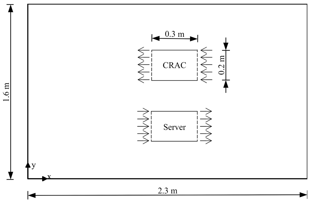
Figure 5. A two-dimensional test case for the boundary conditions.

Airflow was recirculated from the CRAC unit to the server as a closed loop using the boundary conditions developed in the present study. Streamlines and velocity vectors are depicted in Figure 6 and colored according to the local temperature. Hot air recirculation occurred between the IT equipment and CRAC unit. Both boundary conditions exhibited a high stability for the unsteady simulation of the turbulent flow field. BB1 resulted in a higher temperature field than that of BB2 since high temperatures observed at the upper part of the server were increased with a calculated ΔT (Figure 7).

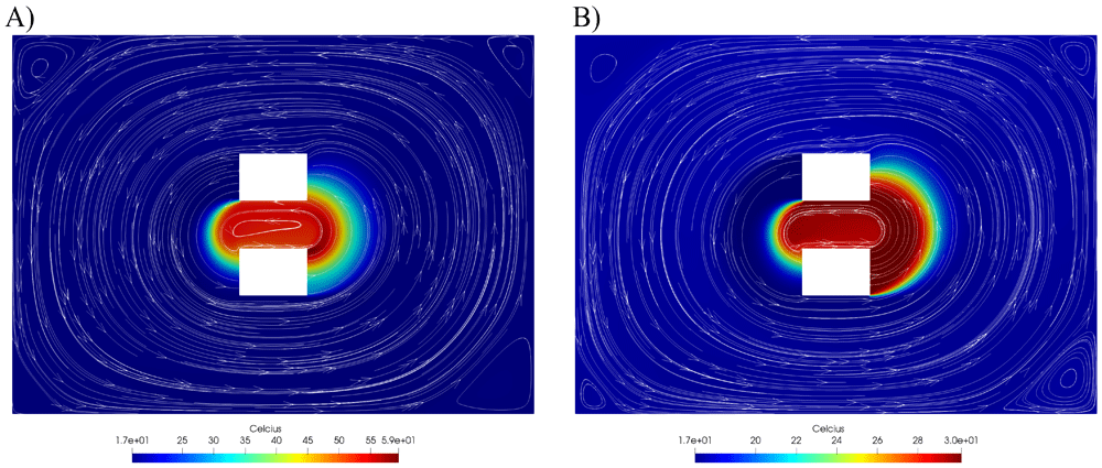
Figure 6.

Streamlines and temperature distribution for (A) BB1 and (B) BB2.

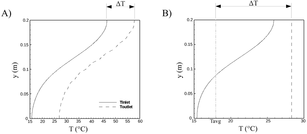
Figure 7.

Temperature profiles at the inlet and outlet of the server for (A) BB1 and (B) BB2.

Temperature profiles at the inlet and outlet of the server are shown in Figure 7 for BB1 and BB2. While the temperature distribution at the inlet was transferred to the outlet with an increment of ΔT in BB1, keeping the temperature profile fixed, average temperature was calculated at the inlet and a uniform temperature profile was applied at the outlet, adding ΔT due to the power consumption by the server. BB2 was suggested for use in the black-box modeling of server components since the temperature profile was not completely preserved by the mixing of the hot and cold parcels inside the server.

Flow in an enclosed environment

Flow and thermal structures in an enclosed environment were investigated by Wang and Chen¹¹ experimentally and numerically for the configuration shown in Figure 8. Dimensions of the room were a= 2.44 m and h=2.36 m, the heights of the inlet and outlet sections were 0.03 m and 0.08 m, respectively. Air entered the room with a fixed velocity of 1.366 m/s and a temperature of 22.2 °C at the inlet and emerged from the outlet of the domain. A cubic box with a side length of 1.22 m was located at the bottom of the room, such that the center of the box coincided with the center of the bottom to create a disturbance in the flow field. Box was heated using a heat source of 700 W and the temperature was measured as 36.7 °C at the surface of the cubic obstacle. The temperature of the surrounding walls was fixed to 27.4 °C during experimental studies.

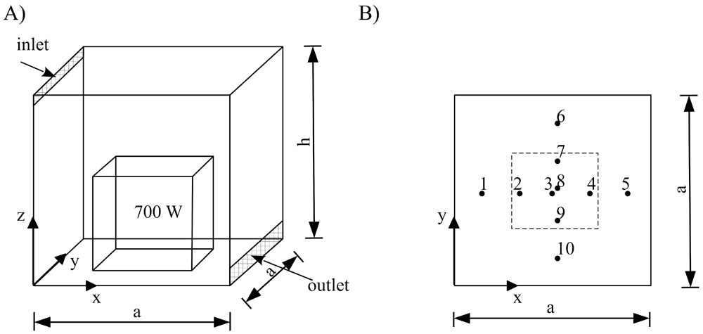
Figure 8.

(A) Three-dimensional view of the room with a heated box and (B) locations of the measurement locations.

Modeling temperature-induced variations of viscosity and density is critical in the numerical simulations of thermal flows. Sutherland’s viscosity law can be used in the thermophysical models of OpenFOAM. Viscosity can be calculated as a function of the temperature in the Sutherland viscosity model:

μ = A_{s} \frac{\sqrt{T}}{1 + T_{s} / T} (23)

Where A_s = 1.4584e-6 [kg m^-1 s^-1 K^-0.5] and T_s = 110.33 [K]. Density can be modeled using the ideal gas law and the Boussinesq approximation:

ρ = \frac{p}{R T} (24)

ρ = ρ_{0} (1 - β (T - T_{0})) (25)

Where ρ₀=1.1839 [kg/m³], β = 3.353e-3 [1/K], T₀ = 298.15 K and R = 287.058 [J/kg K]. Four configurations are defined in Table 4 in order to find the most appropriate thermophysical model for the viscosity and density. Numerical simulations were performed and results were compared with the experimental measurements at different locations in Figure 9 for each configuration. Simulation results show that Configuration 3 produced more accurate results than other configurations.

Table 4. Thermophysical configurations for viscosity and density.

Variable	Configuration 1	Configuration 2	Configuration 3	Configuration 4
μ	Constant μ	Sutherland	Sutherland	Sutherland
ρ	Boussinesq	Boussinesq	Ideal gas	Constant ρ

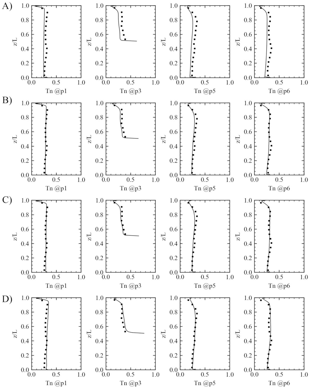
Figure 9. Comparison of temperature profiles with the experimental measurements using different thermophysical models.

(A) Configuration 1, (B) Configuration 2, (C) Configuration 3 and (D) Configuration 4.

Normalized temperature was calculated from the following expression:

T_{n} = \frac{T_{m e a n} - T_{m i n}}{T_{m a x} - T_{m i n}} (26)

Where T_meanis the mean temperature, T_min = 22.2 °C and T_max = 36.7 °C. Simulated normalized velocity (U_n=U/U_max, U_max = 1.5 m/s) profile was compared with the experimental measurements at the location of x=1.2192 m and y= 0.2286 m in Figure 10. The present numerical model captured the vertical variation of the velocity even near the boundaries, which proves that the present wall functions in the turbulence modeling can be reliably used for the modeling of thermal flows in data centers.

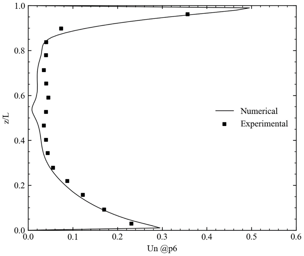
Figure 10. Comparison of the simulated and measured velocities at x=1.2192 m and y=0.2286 m.

Distributions of the velocity vectors and normalized temperature at the midsections of the room are shown in Figure 11. A recirculation region formed at the top of the obstacle due to the separation of the flow from the leading edge, and the separated flow subsequently reattached to form a large recirculation zone. The present numerical model can simulate the buoyancy-driven complex flow structure forming inside the room. Maximum temperatures were observed near the obstacle surfaces. Hence, an upward flow, caused by upward buoyancy forces, is also noticeable in Figure 11. This upward flow increased the recirculation in the region between obstacle and outlet. The heated air was convected towards the cold air jet and mixed with the cold air, forming a hot air zone just above the obstacle. As a result, the mean temperature at the outlet was approximately 4°Chigher than the inlet temperature. As it can be seen in Figure 11, the region between the obstacle and the outlet was exposed to a relatively lower temperature compared to the remaining sides due to the high recirculation and mixing effects.

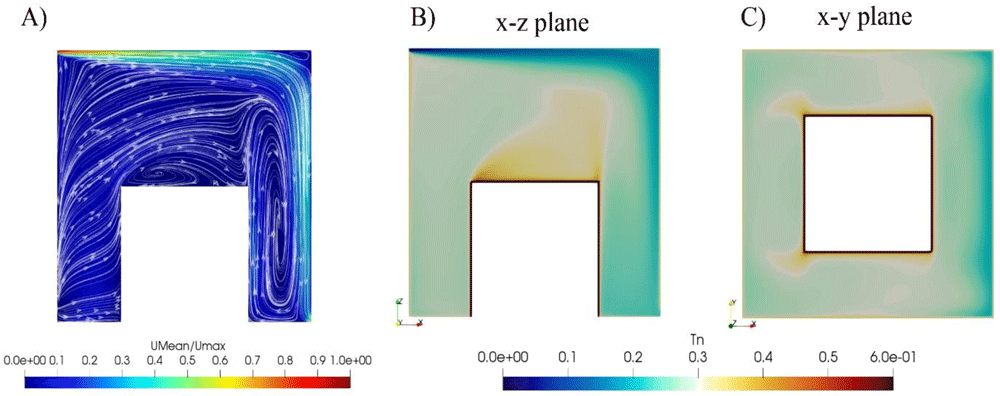
Figure 11.

(A) Velocity vectors and streamlines; temperature distributions at (B) x-z and (C) x-y midplanes of the room.

Forced convection in a room with partitions

Numerical simulation was performed to evaluate the performance of the present numerical model in the forced convection¹². As shown in Figure 12, vertical baffles were located to create different flow regions inside the room¹². The air was supplied from the diffuser located at the inlet with a height of 0.02 m and exhausted at the outlet section with a height of 0.05 m. Experimental measurements were carried along the dashed lines in Figure 12¹².

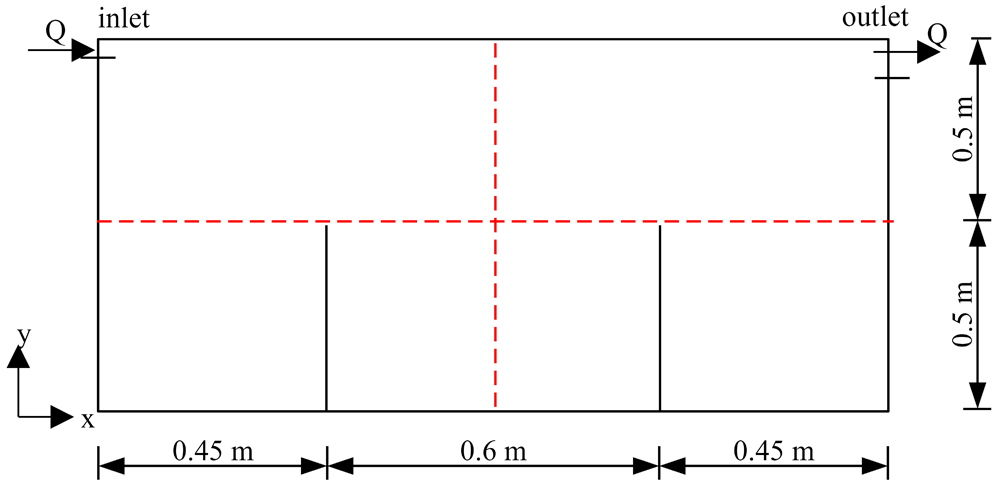
Figure 12. Forced convection in a room with baffles.

Numerical simulations were performed using Re-Normalization Group (RNG); k-ε and k-ω shear stress transport (SST) turbulence models and results are compared with the experimental measurements in Figure 13. As seen in the figure, k-ω SST gave more accurate results than the RNG k-ε turbulence model in a forced convection problem. However, previous numerical simulation results showed that the RNG k-ε turbulence model was more accurate than the k-ω SST model. Such different observations in turbulence models may be due to the wall functions or blending functions used in the k-ω SST model.

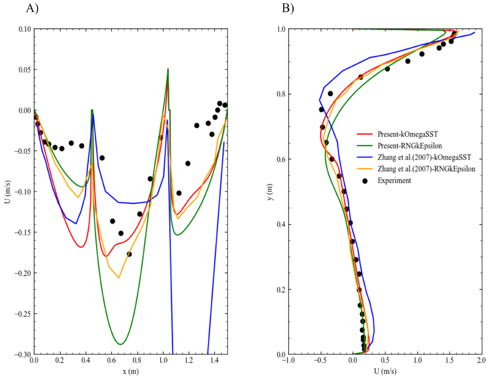
Figure 13. Comparison of the velocity profiles for different turbulence models.

Variation of the velocity profiles with the (A) length and (B) height of the room.

Velocity vectors and streamlines were visiualized based on the mean velocity field in Figure 14. The flow entering the domain followed a thin layer from the inlet to the outlet as a jet flow with high velocities. On the other hand, the separation layer between low and high velocity parcels resulted in the formation of a large recirculation region that occupied most of the domain, and recirculating flow split into three regions due to the existence of vertical baffles. The present numerical model could simulate small recirculation zones forming near the corners of the sub-regions.

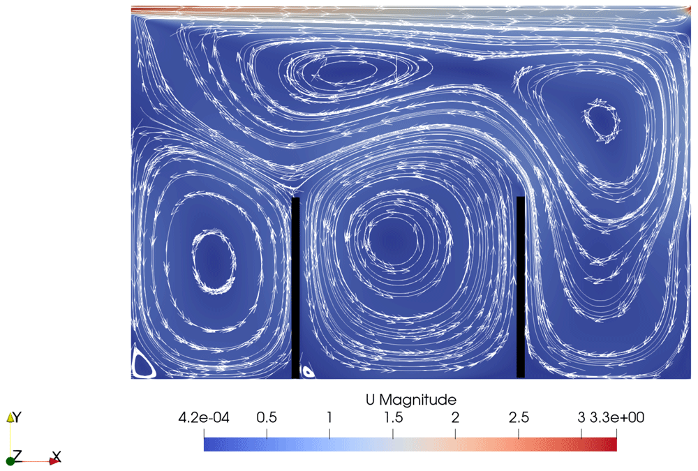
Figure 14. Velocity vectors and streamlines in the room.

Strong natural convection in a model fire room

The case designed by Murakami et al.¹³ was simulated to see the performance of the present numerical model in a strong buoyancy flow. A schematic view of the fire room used in the experimental studies is shown in Figure 15. The heat source located near the corner of the room was 9.1 kW and the average surface temperature measured was higher than 500 °C¹³. The buoyancy-driven flow formed between the room and the opening with dimensions of 0.4 m x 0.9 m x 0.42 m.

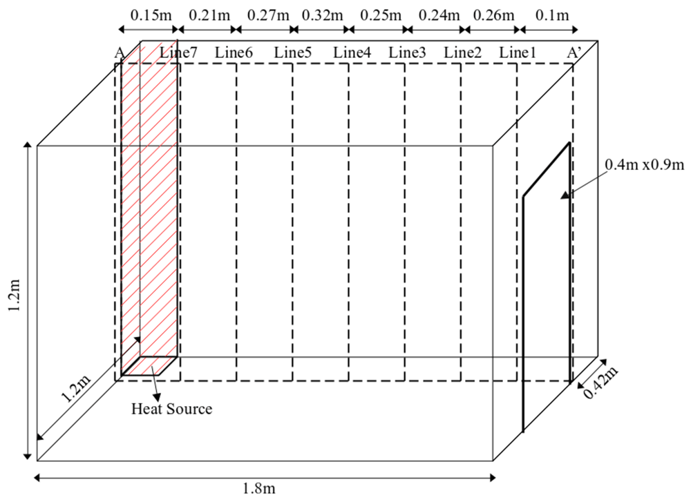
Figure 15. Three-dimensional view of the fire room.

Consistency between numerical and experimental results in Figure 16 proves that the present numerical model can simulate strong buoyancy flows. Representing the physical opening through numerical boundaries was the most crucial step for this test case since the temperature field inside the room was highly sensitive to the outlet boundary conditions. The present outlet boundary conditions allowed both inflow and outflow to the room depending on the calculated fluxes. A fixed velocity of ambient temperature was used when the flow entered the room and a zero-gradient condition was used when the flow emerged from the room. This flexibility of the boundary condition for the temperature at the opening gave accurate results without defining an outer region to see inflow and outflow at the opening.

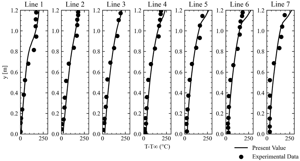
Figure 16. Comparison of the numerical and experimental results at the different locations of the fire room.

Thermal distribution in an open-aisle data center

Thermal distribution in a raised floor open-aisle data center was numerically considered to show the performance of the numerical model on a previously investigated data center¹⁴. As shown in Figure 17, the data center consisted of three racks and two CRAC units for the cooling. Cold air was supplied with a flow rate of 3.04 m³/s from the CRAC1 to the opening located in front of the racks, which is depicted as an inlet. The supply air entered the room at the inlet section and passed through the racks for the cooling of the IT equipment. Rack and tile openings were set to 56% and 25%, respectively, for calculation of the pressure losses through the perforated regions.

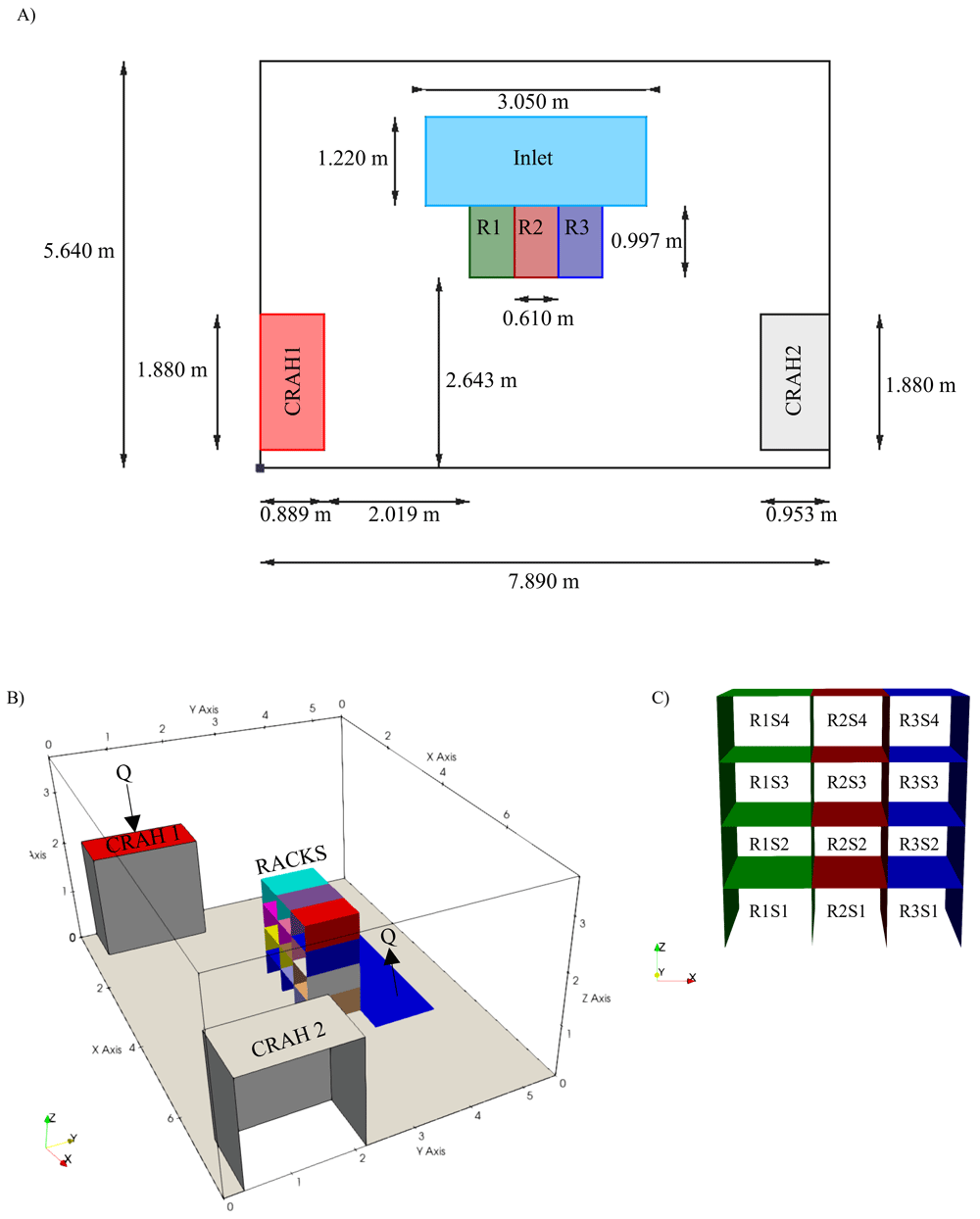
Figure 17.

(A) Plan view, (B) three-dimensional view of the data center and (C) rack layout.

The layout given in Table 5 specifies rack number, starting row of the server in the corresponding rack, height, power consumption and flow rate of the server. The present numerical model read the rack layout from an input file and created corresponding cell zones, heat sources and flow rates for each IT equipment in the open-box model. Such text-based data input is the most common approach used for the labeling of IT equipment in data center applications. Note that racks were numbered from left to right and rows were numbered from bottom to top. It is possible to define server components with different heights (U, 2U, 3U and so on) using the proposed layout structure. After the definition of geometrical properties of the servers, power consumption and flow rate of each server were defined for a working scenario. Different working scenarios can be simulated using the present numerical model for the optimization of the server layout for the energy considerations.

Table 5. Racks layout.

Rack	First row	Height (U)	P (W)	Q (m³/s)
1	1	1	3720	0.31
1	2	1	3720	0.31
1	3	1	3840	0.32
1	4	1	3720	0.31
2	1	1	3645.83	0.35
2	2	1	3645.83	0.35
2	3	1	3854.17	0.37
2	4	1	3854.17	0.37
3	1	1	3809.52	0.32
3	2	1	3690.48	0.31
3	3	1	3809.52	0.32
3	4	1	3690.48	0.31

Unsteady simulation was performed on a mesh consisting of 0.7 million cells for the working scenario defined in Table 5. Time-averaged temperature profiles were compared with the experimental data collected at the front and back of each rack, where variations in temperature field were anticipated to increase significantly. As seen in Figure 18, temperature distribution at the critical locations were captured well using the present computational model.

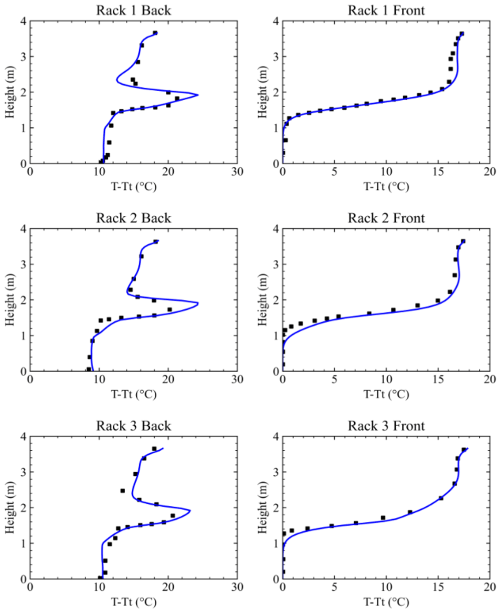
Figure 18. Comparison of the simulation results with the experimental data at the front and back of the racks.

Velocity vectors were visualized in the regions where the local temperatures were lower than the recommended minimum temperature and higher than the recommended maximum temperature in Figure 19 A and B, respectively. The temperature of the supply air was lower than the minimum temperature recommended by the regulations². On the other hand, recirculating flows observed at the top and left of the data center showed significant hot regions where the temperature was higher than the recommended maximum temperature.

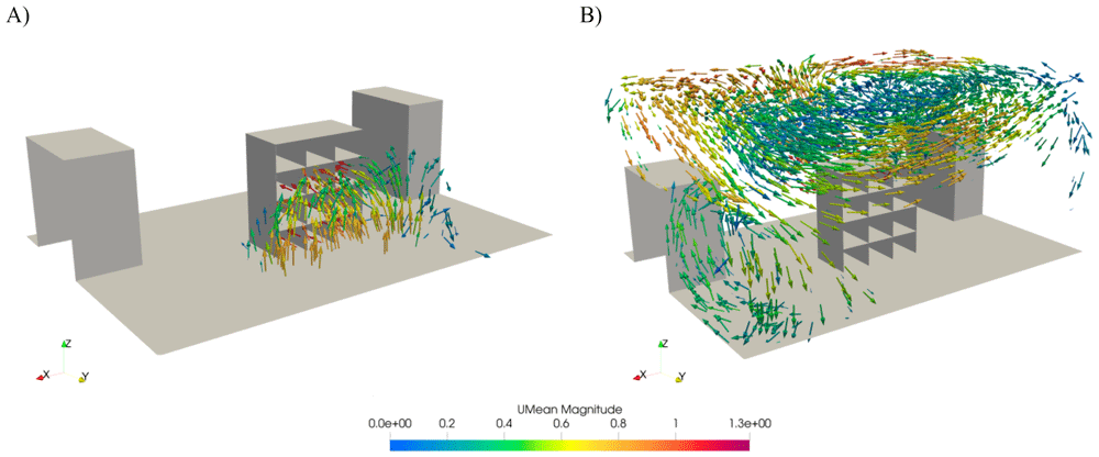
Figure 19.

Velocity vectors in (A) cold and (B) hot regions according to the recommended minimum and maximum temperatures.

Figure 20 shows the temperature distribution at the inlet of the racks. The temperature field near the top of the racks was higher than the maximum recommended temperatures due to the buoyancy effects. Even if increasing discharge of the supply air or decreasing the supply temperature could remedy efficiency-related problems, this increased power consumption by the cooling devices. Thus, the present data center needed to be retrofitted to increase thermal and cooling efficiencies.

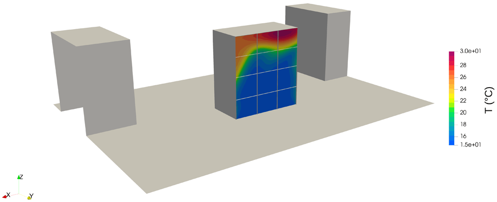
Figure 20. Temperature distributions at the inlet of the rack.

Overall efficiency of the data center was calculated in accordance to the metrics and is shown in Table 6. The RCI_LO indicates a low cooling efficiency since the inlet temperatures of the servers close to the inlet were lower than the recommended minimum temperatures. The RTI shows that the recirculation effects reduced thermal efficiency since the entry of the recirculating flows into the server components increased the maximum temperature.

Table 6. Efficiency metrics for the open-aisle data center.

Efficiency metric	Value	Classification
RCI_HI	99.84%	Good
RCI_LO	31.61%	Poor
RTI	134.44%	Recirculation
SHI	0.96	*
RHI	0.73	**

*Lower SHI values are preferable

**Greater RHI values indicate improved cooling performance, generally acceptable if RHI > 0.8¹⁵

The RCI was calculated for each server component and the distribution of the RCI_LO and RCI_HI are shown in Figure 21. Cooling efficiency decreased at the first and second rows of Rack 2 according to the RCI_LO, which shows an over-cooled region, since the inlet temperatures were lower than the recommended minimum temperatures. Distribution of the RCI_HI shows a slight decrease in the efficiency at the top of Rack 1 due to the hot air recirculation, which was also observed in Figure 20 B. Spatial variations of the efficiency metrics can be determined over the racks using the present numerical model and novel cooling systems can be developed for the detection of low efficient regions.

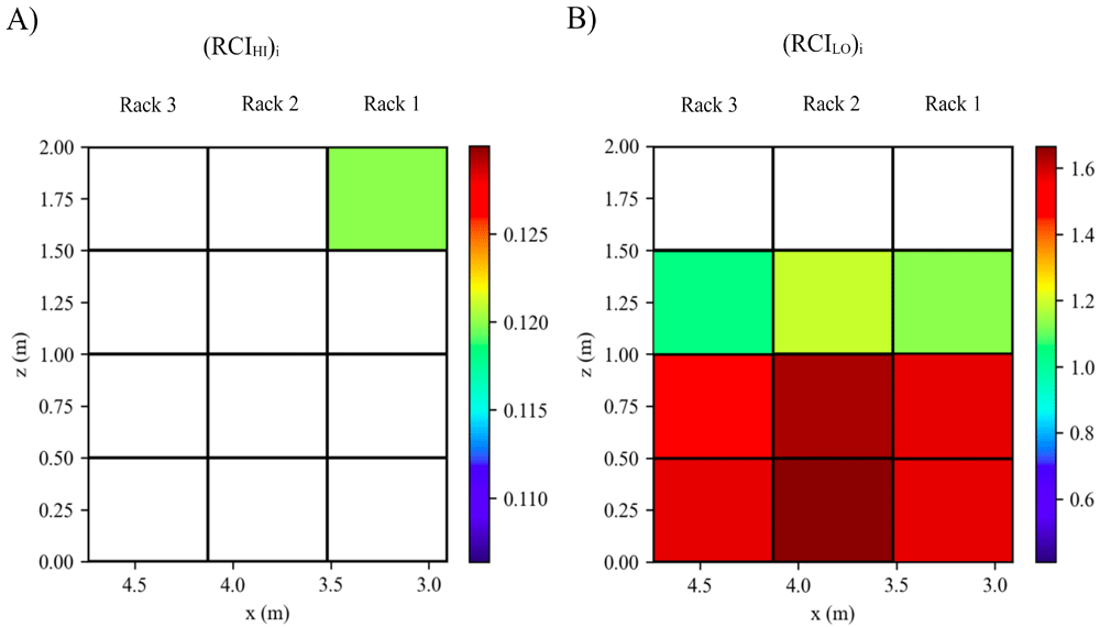
Figure 21. Distributions of the CI_HI and RCI_LO over the racks.

Conclusions

An efficient cooling system is required for data centers to enhance energy and cooling efficiencies. Numerical and experimental studies conducted in the literature have increased our understanding of enhanced airflow performance of a data center at the design stage. CFD is widely used in the thermal design of data centers. In this study, an open-source CFD model was developed based on OpenFOAM libraries for the efficiency assessment of air-cooled data centers. The model was validated with the experimental measurements conducted in an enclosed thermal environment, forced convection in a room and strong buoyancy flow in a fire room. Then, thermal distribution in an open-aisle data center was simulated for a working scenario of 45 kW. The consistency observed between numerical results and experimental data shows that the present numerical model can accurately predict thermal distribution in a real data center. The proposed layout structure enables to perform a series of numerical simulations for different thermal scenarios, which is fundamental to the development of artificial intelligence (AI)-based cooling systems. The present computational model can also calculate efficiency metrics for each server component individually. Distribution of the metrics over the rack layout enables to capture critical zones where thermal and cooling efficiencies decrease due to the hot air recirculation and cold air by-pass. OpenFOAM casesare publicly distributed to increase the dissemination of the study.

Data availability

Underlying data

The scripts generated and used during the present study are not publicly available due to the fact that the ECO-Qube Grant Agreement (Agreement number: 956059) obliges project partners to protect the results which have the potential to be commercially exploited. The CFD scripts are related to Deliverable 2.2 "Open Source CFD Model" of the ECO-Qube Project, where protection requirements were agreed upon with the contracting authority and the deliverable dissemination level was set to confidential. Therefore, we cannot disseminate these results which have commercialization potential.

Extended data

Zenodo: OpenFOAM cases of the paper "Development and validation of an open-source CFD model for the efficiency assessment of data centers", https://doi.org/10.5281/zenodo.6336674¹⁶

This project contains the following underlying data:

Validation1.tar.xz (contains OpenFOAM files and scripts for the simulation of flow and thermal structures in an enclosed environment¹¹).
Validation2-kOmegaSSTModel.tar.xz (contains OpenFOAM files and scripts for the simulation of forced convection in a room¹² using k-omega SST turbulence model.)
Validation2-RNGkEpsilonModel.tar.xz (contains OpenFOAM files and scripts for the simulation of forced convection in a room¹² using RNG k-epsilon turbulence model.)
Validation3.tar.xz (contains OpenFOAM files and scripts for the simulation of strong natural convection in a model fire room¹³)
Validation4.tar.xz (contains OpenFOAM files and scripts for the simulation of thermal distribution in an open-aisle data center¹⁴)
Results_Validation1.tar.xz (Simulation results of the Validation case 1.)
Results_Validation2.tar.xz (Simulation results of the Validation case 2.)
Results_Validation3.tar.xz (Simulation results of the Validation case 3.)
Results_Validation4.tar.xz (Simulation results of the Validation case 4.)
layout.csv (Input file for the Validation case 4.)

Data are available under the terms of the Creative Commons Attribution 4.0 International license (CC-BY 4.0).

Acknowledgements

All intellectual property rights are owned by ECO-Qube consortium members and are protected by the applicable laws. Reproduction is not authorised without prior written agreement.

The commercial use of any information contained in this document may require a license from the owner of that information.

The funders had no role in study design, data collection and analysis, decision to publish, or preparation of the manuscript.

The opinion stated in this deliverable reflects the opinion of the authors and not the opinion of the European Commission.

Faculty Opinions recommended

References

1. Emerson Network Power: Energy logic: reducing data center energy consumption by creating savings that cascade across systems, A White Paper from the Experts in Business-Critical Continuity. Reference Source
2. ASHRAE TC 9.9: Thermal Guideline for Data Processing Environments. American Society of Heating Refrigerating and Air-Conditioning Engineers. Inc.: Atlanta, GA USA, 2015.
3. Cho J, Yang J, Park W: Evaluation of air distribution system's airflow performance for cooling energy savings in high-density data centers. Energy Build. 2014; 68(Part A): 270–279. Publisher Full Text
4. Nada SA, Said MA: Effect of CRAC units layout on thermal management of data center. Appl Therm Eng. 2017; 118: 339–344. Publisher Full Text
5. Davidson PA: Turbulence: An introduction for scientists and engineers. Oxford University Press, New York. 2004. Reference Source
6. Sheth DV, Saha SK: Numerical study of thermal management of data centre using porous medium approach. J Build Eng. 2019; 22: 200–215. Publisher Full Text
7. Kuwahara F, Kameyama Y, Yamashita S, et al.: Numerical modeling of turbulent flow in porous media using a spatially periodic array. J Porous Media. 1998; 1(1): 47–55. Publisher Full Text
8. Herrlin MK: Airflow and cooling performance of data centres: two performance metrics. ASHRAE Tran. 2008; 114(2): 182–187. Reference Source
9. Sharma R, Bash C, Patel C: Dimensionless parameters for evaluation of thermal design and performance of large-scale data centres. 8th AIAA/ASME Joint thermophysics and heat transfer conference. 2002. Publisher Full Text
10. Han X, Tian W, VanGilder J, et al.: An open source fast fluid dynamics model for data center thermal management. Energ Buildings. 2021; 230: 110599. Publisher Full Text
11. Wang, M, Chen Q: Assessment of Various Turbulence Models for Transitional Flows in an Enclosed Environment (RP-1271). HVAC&R Res. 2009; 15(6): 1099–1119. Publisher Full Text
12. Zhang Z, Zhang W, John Z, et al.: Evaluation of Various Turbulence Models in Predicting Airflow and Turbulence in Enclosed Environments by CFD: Part 2—Comparison with Experimental Data from Literature. HVAC&R Res. 2007; 13(6): 871–886. Publisher Full Text
13. Murakami S, Kato S, Yoshie R: Measurement of turbulence statistics in a model fire room by LDV. ASHRAE Trans. 1995; 101(2): 287–301. Reference Source
14. Abdelmaksoud WA, Dang TQ, Ezzat Khalifa H, et al.: Improved computational fluid dynamics model for open-aisle air-cooled data center simulations. J Electron Packag. 2013; 135(3): 030901–30913. Publisher Full Text
15. Norouzi-Khangah B, Mohammadsadeghi-Azad MB, Hoseyni SM, et al.: Performance assessment of cooling systems in data centers; Methodology and application of a new thermal metric. Case Stud Therm Eng. 2016; 8: 152–163. Publisher Full Text
16. Dogan A, Yilmaz S, Kuzay M, et al.: OpenFOAM cases of the paper "Development and validation of an open-source CFD model for the efficiency assessment of data centers" [Data set]. Zenodo. In Open Research Europe (Version 2) 2022.

Comments

Publication information

Section

Method Article

Published

March 24, 2022

DOI

https://doi.org/10.12688/openreseurope.14579.1

Versions

March 24, 2022 (Published Manuscript Under Review 1.0)

Included in

Funding data

European Commission

Grant ID(s): 956059

Metrics

Views

362

Downloads

Citations

See full metrics

Keywords

Data center, cooling efficiency, thermal structure, efficiency assessment, CFD, OpenFOAM

Comments

Aras Dogan

Design and Simulation Tech. Inc, Eskisehir, 26480, Turkey

Roles

Co-Author, Formal Analysis, Investigation, Methodology, Resources, Software, Validation, Visualization, Writing – Original Draft Preparation

0000-0001-8768-2056

aras.dogan@dstechno.net

Sibel Yilmaz

Design and Simulation Tech. Inc, Eskisehir, 26480, Turkey

Roles

Co-Author, Data Curation, Formal Analysis, Methodology, Resources, Software, Validation, Visualization, Writing – Original Draft Preparation

0000-0002-3261-2605

sibel.yilmaz@dstechno.net

Mustafa Kuzay

Design and Simulation Tech. Inc, Eskisehir, 26480, Turkey

Roles

Co-Author, Formal Analysis, Investigation, Methodology, Resources, Software, Validation, Visualization, Writing – Original Draft Preparation

0000-0002-6205-4819

mustafa.kuzay@dstechno.net

Ender Demirel

Design and Simulation Tech. Inc, Eskisehir, 26480, Turkey

Eskisehir Osmangazi University, Eskisehir, 26480, Turkey

Roles

Corresponding Author, Co-Author, Conceptualization, Data Curation, Funding Acquisition, Investigation, Methodology, Project Administration, Resources, Supervision, Writing – Original Draft Preparation, Writing – Review & Editing

0000-0002-0440-7866

edemirel@dstechno.net

Downloads over the last 12 months:

Cited by

via Crossref

View citing articles

[1] 1. Emerson Network Power: Energy logic: reducing data center energy consumption by creating savings that cascade across systems, A White Paper from the Experts in Business-Critical Continuity. Reference Source

[2] 2. ASHRAE TC 9.9: Thermal Guideline for Data Processing Environments. American Society of Heating Refrigerating and Air-Conditioning Engineers. Inc.: Atlanta, GA USA, 2015.

[3] 3. Cho J, Yang J, Park W: Evaluation of air distribution system's airflow performance for cooling energy savings in high-density data centers. Energy Build. 2014; 68(Part A): 270–279. Publisher Full Text

[4] 4. Nada SA, Said MA: Effect of CRAC units layout on thermal management of data center. Appl Therm Eng. 2017; 118: 339–344. Publisher Full Text

[5] 5. Davidson PA: Turbulence: An introduction for scientists and engineers. Oxford University Press, New York. 2004. Reference Source

[6] 6. Sheth DV, Saha SK: Numerical study of thermal management of data centre using porous medium approach. J Build Eng. 2019; 22: 200–215. Publisher Full Text

[7] 7. Kuwahara F, Kameyama Y, Yamashita S, et al.: Numerical modeling of turbulent flow in porous media using a spatially periodic array. J Porous Media. 1998; 1(1): 47–55. Publisher Full Text

[8] 8. Herrlin MK: Airflow and cooling performance of data centres: two performance metrics. ASHRAE Tran. 2008; 114(2): 182–187. Reference Source

[9] 9. Sharma R, Bash C, Patel C: Dimensionless parameters for evaluation of thermal design and performance of large-scale data centres. 8th AIAA/ASME Joint thermophysics and heat transfer conference. 2002. Publisher Full Text

[10] 10. Han X, Tian W, VanGilder J, et al.: An open source fast fluid dynamics model for data center thermal management. Energ Buildings. 2021; 230: 110599. Publisher Full Text

[11] 11. Wang, M, Chen Q: Assessment of Various Turbulence Models for Transitional Flows in an Enclosed Environment (RP-1271). HVAC&R Res. 2009; 15(6): 1099–1119. Publisher Full Text

[12] 12. Zhang Z, Zhang W, John Z, et al.: Evaluation of Various Turbulence Models in Predicting Airflow and Turbulence in Enclosed Environments by CFD: Part 2—Comparison with Experimental Data from Literature. HVAC&R Res. 2007; 13(6): 871–886. Publisher Full Text

[13] 13. Murakami S, Kato S, Yoshie R: Measurement of turbulence statistics in a model fire room by LDV. ASHRAE Trans. 1995; 101(2): 287–301. Reference Source

[14] 14. Abdelmaksoud WA, Dang TQ, Ezzat Khalifa H, et al.: Improved computational fluid dynamics model for open-aisle air-cooled data center simulations. J Electron Packag. 2013; 135(3): 030901–30913. Publisher Full Text

[15] 15. Norouzi-Khangah B, Mohammadsadeghi-Azad MB, Hoseyni SM, et al.: Performance assessment of cooling systems in data centers; Methodology and application of a new thermal metric. Case Stud Therm Eng. 2016; 8: 152–163. Publisher Full Text

[16] 16. Dogan A, Yilmaz S, Kuzay M, et al.: OpenFOAM cases of the paper "Development and validation of an open-source CFD model for the efficiency assessment of data centers" [Data set]. Zenodo. In Open Research Europe (Version 2) 2022.

Development and validation of an open-source CFD model for the efficiency assessment of data centers

List of Authors

Peer review

Publication information

Included in

Funding data

Metrics

Keywords

Comments

Abstract

Comments

Publication information

Included in

Funding data

Metrics

Keywords

Comments

Authors & roles

Aras Dogan

Sibel Yilmaz

Mustafa Kuzay

Ender Demirel

Downloads over the last 12 months:

Cited by

via Crossref