Plain language summary
Geographic Information Systems (GIS) are built over geospatial databases that represent geographic features as abstract geometric shapes (points, lines, polygons) where queries about shape intersection, inclusion, and proximity can be efficiently processed. These queries can be specific (e.g., “find all carparks within 5km from here”) or open, analytical queries where (potentially) all shapes need to compared against all other shapes (e.g., “find all cities that are within 5km of a lake”). Intuitively, we expect the time to calculate the distance between two shapes to increase for more complex polygons, since a larger number of comparisons between the elements of the shapes needs to be performed. In the context of an analytics queries that need to compare thousands of cities against thousands of (potentially) matching lakes, this can have a detrimental effect on the responsiveness of the database. Databases optimize query execution by pruning shapes that cannot possibly be within the specified distance from each other before computing the exact distance. For this, they use the “bounding box” of each shape which can be both very efficiently found and very efficiently compared with other bounding boxes.
Our method adds a second pruning step, where bounded boxes are used to find shapes that are guaranteed to satisfy the filter, regardless of what the exact distance is. Our experiments found that there is too small a difference in the time it takes to compute the distance between a complex polygon and a point versus a rectangle and a point. This went counter to intuition so, upon deeper investigation, we found that PostGIS applies an (undocumented in academic literature) optimization to calculate the distance between shapes. This leaves too small a margin to perform any meaningful optimization, although our method in shown to work correctly and efficiently.
Introduction
In geospatial query processing, some queries (such as spatial containment and intersection) can be efficiently answered from the index. There are other queries (such as within-distance), however, that suggest that every shape in the database is a potential match and should, in principle, be considered as candidate and compared with the threshold. Certainly, this is impractical and optimizations have been developed that efficiently reduce the set of candidate shapes before starting to actually compute distances and apply the threshold.
In the case of the within-distance queries, many candidates can be eliminated in advance as too distant. Geospatial databases already use a first direct optimization, since they organize data as a hierarchy of minimum bounding boxes; the actual distance between two shapes cannot be smaller than the distance between their bounding boxes.
Nevertheless, not all shape configurations give bounding boxes that are selective for nearby shapes. More concrete, these configurations may result outside the requested distance from an actual shape but within the requested distance from its bounding box. In this article, we investigate a further optimization, envisaged as a second step after minimal bounding boxes elimination and before computing precise distances. Specifically, we investigate using maximal bounded boxes to identify candidates that are guaranteed to satisfy the threshold, leaving an even smaller set of candidates where distances need to be computed.
In the remainder of this article we first provide the relevant Background, including both approximation-based optimizations and the optimizations performed by PostGIS to calculate the exact distance. We then present our Motivation based on the limitations observed in the literature; and then proceed to present our Maximal Bounded Approximations approach. We finally present Evaluation results and Conclusions.
Background
In this section we first give some background information on the structure of spatial objects and the indexes used on them. We will investigate typical strategies of spatial joins and ideas used for improving their performance, and specifically the distance operator. Then we will describe how the distance operator is implemented in PostGIS, and we will investigate approaches using shape approximations to speed up spatial topological relation queries.
Spatial objects, indexes and joins
A spatial object contains at least one spatial attribute that describes the geometry of the object. This attribute consists of two- or three-dimensional geometric data that include simple primitive elements, such as points, lines, curves, rectangles, polygons (with or without holes), surfaces, and even more complex types made up of a combination of the primitive elements. In this work, we investigate spatial join processing for two-dimensional spatial objects whose geometry correspond to polygonal areas. The geometry is assumed to be in vector representation, i.e., it is given as a sequence of two-dimensional points. The indexes used on these polygonal areas are using either vector (maximum enclosed rectangles) or raster approximations (grid cells).
A spatial query is related to the geometric attribute of the spatial object. A typical spatial query is the window query where the response set consists of all objects whose geometric component overlaps with a given rectilinear query rectangle. Spatial joins, on the other hand, are defined on two or more relations. They find all pairs of objects from these relations that satisfy a given spatial predicate according to their geometric attributes, such as intersection. For example, consider the spatial relations Rivers (Id, Name, RRegion) and Cities (Id, Name, CRegion). The geometric attributes RRegion and CRegion represent the borders of rivers and cities, respectively. A spatial join answers queries such as “find all cities that are crossed by a river”. Here the spatial join is on the relations Rivers and Cities, and the spatial predicate is whether a river intersects a city.
Typically, spatial joins (i.e. point-polygon, line-polygon, polygon-polygon joins) follow a two-phase evaluation strategy, known as the filter and refine approach1. During the filtering phase an index (i.e. an R-tree, which is the most widespread spatial access method) is usually used on the minimum bounding rectangles (MBRs) of polygons. The objects that could not possibly satisfy the query are pruned, in order to obtain a list of candidate join pairs. This step can be efficiently supported by spatial access methods such as R-trees2, quad trees3 etc. Minimum bounding rectangles (MBRs, also known as minimum bounding boxes (MBBs) or envelopes) are preferred over the full objects because they require less memory, and intersections between them are easier to calculate4. In the refinement phase, expensive tests are performed on the exact objects to discard false matches and retrieve the actual solutions.
For most spatial datasets, spatial objects typically have descriptions that consist of hundreds or thousands of vertices and are complex. Spatial datasets themselves are also typically large, containing thousands or millions of objects. Reading a large amount of objects from external memory and performing join tests on them can be extremely expensive in terms of input/output (I/O) performance4. Therefore, during spatial joins, some of the most expensive operations are to transfer the large data geometries from external to main memory (loading cost) and to compute the join predicate of spatial objects (comparison cost). For point datasets the loading cost dominates, while for polygon datasets both costs contribute significantly.
Turning our attention to spatial indexing, we observe that R-trees are height-balanced trees oriented in reducing the number of disk accesses and saving time in reaching any data object. The non-leaf nodes contain shape approximations (usually MBRs) with all the objects contained in their child nodes. The leaf nodes contain pointers to actual data objects. R-trees are designed so that visiting only a small number of nodes suffices to reach a leaf node.
The key difficulty of R-trees is to build an efficient tree that on one hand is balanced, so the leaf nodes are at the same level. And on the other hand the rectangles do not cover too much empty space and do not overlap too much, so that during search, fewer subtrees need to be processed. For example, the original idea for inserting elements to obtain an efficient tree is to always insert into the subtree that requires least enlargement of its bounding rectangle.
When data is organized in an R-tree, the neighbors within a given distance of all points can efficiently be computed using a spatial join5. Also, the R-tree structure minimizes the cost in computing the distance between two data objects, as all non-leaf nodes contain MBRs with the minimum portion of dead space. Nonetheless, the distance operator is one of the most expensive geometric operations.
A large body of work has been done6–10 in order to improve the performance of spatial joins. As R-trees are constructed in a way to create nodes that are as close as possible to the actual measures of the objects they contain, there is no need for a further optimization in the spatial access method.
Generally, the main goal is to accelerate expensive steps (refinement) by preceding more cheap steps (filtering) which reduce the number of spatial objects investigated in an expensive step. After using spatial access methods on MBRs, another intermediate step could be added to further restrict the search space and postpone processing the exact representation of the spatial objects, or even bypass it. This is usually achieved by using additional approximations (i.e., inner rectangles) to approximate the interior of polygons or reduce the dead space in cells. In contrast to exterior approximations, interior approximations do not include extra dead space, but rather exclude portions of the full object. Certainly, this comes at the cost of higher memory consumption than filter and refine approaches. However, nowadays we can actually afford this higher memory consumption in exchange for higher performance.
In theory, in operations such as computing distance between objects, the use of minimum bounding rectangles followed by another filtering step (i.e. maximum bounded rectangles, or grid approximations with limited dead space in cells) would greatly reduce the number of distance operations between actual object geometries needed to be done. In the following subsections we will first describe how the distance operator is implemented in PostGIS. Then we will investigate approaches using shape approximations to speed up spatial topological relation queries.
PostGIS (within-)distance operator
Implementation In PostGIS the distance between two 2-dimensional is calculated as follows:1
1. For two 2-dimensional shapes, excluding points, check if their minimum bounding boxes overlap. If they are disjoint continue to step 2. If they overlap, of at least one shape in a point, continue to step 17.
2. Calculate the center-center c1-c2 line of the bounding rectangles, where c1(x1, y1) is the center of the first bounding rectangle and c2(x2, y2) of the second.
3. Calculate the deltaX and deltaY of the centers of the bounding rectangles, with the following equations:
5. Create two lists with the sorted z-values and their corresponding points; one for each shape.
6. Calculate the distance of each center point to the origin axes. If deltaX2 < deltaY2 use Equation 6, otherwise use Equation 7.
7. Find the shape closer to the origin axes. If c1m < c2m the first shape is closer to the origin axes, otherwise the second shape is closer.
8. Find distance dist between the first points of the two lists.
9. For the shape closer to the origin axes keep the last z-value zA in the sorted list (further from the origin axes) and its corresponding vertex A.
10. For the shape further from the origin axes keep the first z-value zB in the sorted list (closer to the origin axes) and its corresponding vertex B.
11. Compute maxmeasure using dist:
12. If the difference between the two z-values is greater than maxmeasure (zB − zA > maxmeasure) then break.
13. If distance between A and B is less than dist, replace dist.
14. Check the segment before and after points A and B. If distance between A and the one of the two segments starting from B is less than dist, replace dist. Similarly, if distance between B and the one of the two segments starting from A is less than dist, replace dist.
15. Repeat from step 11 with the next B and zB of the second list. If there is no next element, keep the first element again and continue to the next step.
16. Repeat from step 11 with the previous A and zA of the first list. Break if both lists have been traversed.
17. Perform a brute-force distance calculation, according to the type of each shape. Assume that, without loss of generality, the shapes are both polygons; let as name them A and B.
18. If polygon A has its first point outside of polygon B and vice versa, just check the outer rings in step 22.
19. If the first point of polygon B is in a hole of polygon A, check the outer ring of polygon B against that specific hole of polygon A in step 22.
20. If the first point of polygon A is in a hole of polygon B, check the outer ring of polygon A against that specific hole of polygon B in step 22.
21. If none of the above stands, it means that the first point of one of the polygons is inside the outer ring of the other, so dist = 0.
22. Calculate distance from each line segment of the one shape against each segment of the other shape.
If the shape is a collection repeat from step 1 to calculate the distance for every possible combination of sub-geometries.
The within-distance operator uses the implementation described above but returns immediately when the calculated distance drops below a specified tolerance.2 Having said that, one can easily notice that PostGIS uses an approximation of the actual distance calculation to compute the within-distance operator. Consequently, the execution time of the within-distance operator is further reduced.
Conclusions
As a result of the PostGIS distance and within-distance implementation the execution time of the distance operator between two shapes, excluding points, whose minimum bounding rectangles do not overlap is not completely dependent on the complexity of the shapes. In most cases only a few vertices of each shape are needed for calculating the distance. For more complex shapes, the additional delay is caused by calculating the z-values and sorting the lists containing them. For the within-distance operator even fewer vertices are needed; when distance reaches a specified threshold no further calculations are needed. Consequently, the number of vertices should not significantly affect the execution time of the distance operator, let alone the execution time of the within-distance operator.
We are going to experimentally test whether this small dependence on polygon complexity leaves an optimization margin. That is, whether using a simpler approximation for complex polygons can out-perform the standard PostGIS implementation.
Shape approximations
As mentioned before there is a large amount of work done in order to improve the performance of spatial joins. For convex polygons, the operation finding the enclosed rectangles is trivial and in many cases only one bounded rectangle suffices to cover the largest area of each polygon. In more complex cases, where a polygon is concave, more than one bounded rectangle is required for each polygon. These multiple bounded rectangles should cover a large amount of the surface of the polygon. Another approximation for spatial indexing, apart from maximum bounded rectangles, is the grid approximation. In this approximation, space is divided into cells and the spatial data value is represented by the set of cells that the object intersects. With this approximation the chosen cells contain the whole area of the object as well as some dead space. Below, we investigate some of the approaches using additional approximations before the refinement step, to speed up spatial topological relation queries.
More accurate exterior approximations (i.e. rotated minimum bounding rectangles (RMBRs), convex hull, minimum bounding m-corner (m-C), circles (MBCs) and ellipses (MBEs)) can be used additionally to minimum bounding rectangles, in order to further filter out false hits6. Following the filter-and-refine approach a set of candidates would be computed performing the MBR-join between all geometries. Then a join on more accurate approximations on the candidate set would be performed excluding more polygons before the exact geometries need to be accessed.
Interior approximations can also be used to detect hits in the candidate set without still accessing the exact geometries. Some interior approximations for convex polygons are the maximum enclosed rectangles (MERs) and circles (MECs)6. If the join queries on these approximations are successful, i.e. the interior approximations of two geometries intersect, then the exact geometries also intersect. The refinement phase is reached only in cases where the queries above fail.
Several algorithms exist for the computation of a maximal interior rectangle for convex polygons, starting from O(n log2n)- time11 and then improved to O(n log n)12. Given the list vertices of a convex polygon in counterclockwise order and stored in a balanced binary search tree, the approaches compute the maximal axis-aligned interior rectangle.
If the vertices of the minimum bounding rectangle of the candidate geometry are inside the maximal enclosed rectangle (or any of the interior approximations) of the convex polygon geometry, then the candidate geometry is inside the convex polygon geometry. This assumption cannot be made for concave polygons, due to the fact that their inner approximations might not be contiguous. The computation of a maximal interior rectangle for concave polygons is much more challenging due to their complex form and their large amount of vertices. Their inner rectangles could be quite large, in the order of hundreds or even thousands.
A technique to overcome those challenges is to tile the concave geometry similarly to the quad-tree decomposition, using the minimum bounding rectangle of the concave polygon as the gridding domain8. Each time the gridding level increases, each cell is subdivided into four sub-quadrants. The amount of the inner cells of the concave geometry increases, resulting in reduction in response time (due to skipping the refinement-step comparisons), but also in the increase of the overall overhead (due to the cost of fragmenting the minimum bounding rectangle to the specified level). An x-ordered and a y-ordered array containing the inner cells are used to determine whether the concave geometry contains the candidate geometry or not. If all four vertices of the minimum bounding rectangle of the candidate geometry are inside the inner cells of the concave polygon then the candidate polygon might lie within the concave polygon. For each edge of the minimum bounding rectangle, its length is compared to the number of cells contained between its endpoints (i.e. amount of cells in the y-ordered array for edges parallel to the x-axis). If they are equal the edge is considered to be inside the geometry, otherwise not.
For another quad-tree-based approximation, the minimum bounding rectangle of each shape is decomposed into a four level hierarchy of axes-aligned grids9. Each of the four levels can have a different grid division setting, resulting in diverse grid densities. A two-dimensional boolean array is computed for every object to indicate for each cell if the object touches, partially or fully covers it. The quad-tree-like multi-level grid and the boolean array are used as a step trying to avoid invoking the computationally expensive spatial filter method.
Other approaches use raster approximations, i.e. the four-color raster approximation7. Such approaches consists of keeping a raster approximation for the MBR of each polygon, containing cells. Each cell contains two bits of information to indicate the percentage of the cell occupied by the polygon (i.e. the cell does not intersect the polygon, more than 50% is covered by the polygon, less than 50% is covered, the cell is fully covered). In order to check if two polygons intersect, their raster approximations in the area where their MBRs intersect should be superimposed. If both the superimposed cells are covered by more than 50% by their polygon then the polygons intersect. If one superimposed cell is fully covered and the other is partly covered (i.e. by either more or less than 50%), then the polygons also intersect. If one of them is not covered at all then it is certain that the polygons do not intersect. The only inconclusive cases are when the one superimposed cell is covered by less than 50% by its polygon and the other is partly covered. In such cases the polygons remain candidate polygons and a refinement step is needed.
A more novel approach10 does not use the minimum bounding rectangles of the polygons in order to reduce the number of candidate polygons. It creates a universal grid and computes cell-based approximations (interior and boundary) of all polygons. All grid cells are disjoint so that each point belongs to at most one cell. Therefore, two or more polygons could overlap in a single cell, and a point could intersect with multiple polygons. The produced grid can be very coarse-grained in interior and very fine-grained in boundary areas. This approach concentrates in point-in-polygons tests, so maintaining intersecting cells would result in points intersecting with more than one cells, which would reduce the lookup performance.
In conclusion, several algorithms exist for the computation of interior approximations. For convex polygons the computation of maximal interior rectangles is trivial. For concave polygons computing good grid approximations is much more challenging, due to the complexity of the shapes. Based on the above, there is no commonly accepted most-efficient inner approximation for concave shapes. In the following section we present our motivation for the current work based on the limitations observed in the literature.
Motivation
Some approximations use singe-resolution grids8, while others handle multiple levels of resolution7,9,10. In most approaches the approximations are created for each polygon individually7–9, while the idea of using a single universal grid is also proposed10. All of these approaches introduce some limitations in the computation of the interior approximations. In this section we are going to investigate some of these limitations introduced by the approaches described in the previous section, and describe our motivation for the current work based on them.
In Figure 1 we can see the interior approximation, specifically the maximum enclosed rectangle of a polygon6. It is quite clear that only a small portion of the overall area of the polygon is covered. Therefore, instead of computing a single maximum enclosed rectangle for each polygon, we propose an approach that offers a maximal area coverage with multiple rectangles at the cost of consuming a little more memory. Note that concave polygons need more interior rectangles to cover the same area percentage covered by a single rectangle in the case of convex polygons. Following the same reasoning, concave polygons with more reflex interior angles (like in Figure 6a) are likely to need more interior rectangles than the simpler ones.
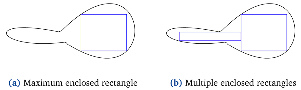
Figure 1. Single maximum enclosed rectangle and multiple enclosed rectangles of a polygon.
According to the most novel approach described in the previous section, all inner rectangles of a geometry should be disjoint so that each geographical point would belong to at most one of them10. While in point-in-polygon tests intersecting cells might reduce the lookup performance, in the representation of the interior of a polygon intersecting cells would probably cover more area, as shown in Figure 2. The approach we have in mind suggests covering maximal interior area of a polygon while using minimal possible rectangles. This contradicts the notion that all inner cells should be disjoint. If, for example, we want to cover the same area in Figure 2a and Figure 2b, with disjoint and intersecting rectangles respectively, then we would require three rectangles in the former case and two in the latter.
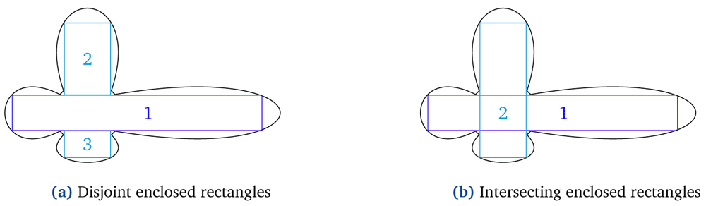
Figure 2. Disjoint versus intersecting enclosed rectangles of a polygon.
Figure 3 illustrates fragmented versus contiguous interior approximations. Specifically, we can see the drawbacks of using fragmented rectangles8 as an approximation for concave polygons. The vertices of both the green and the red boxes3 (i.e. minimum bounding rectangles of some candidate geometries) are contained in the inner pieces of the concave geometry. In the case where the interior approximations are fragmented it is not safe to assume any correlation between the containment of the vertices of each box and the actual containment of the box inside the concave polygon. A candidate geometry might intersect with multiple inner pieces of the concave polygon and still not be completely inside the concave polygon. On the contrary, when the interior approximations are contiguous the conclusion that some of the candidate geometries (i.e., the red minimum bounding rectangle) are completely inside the concave polygon can be safely made.
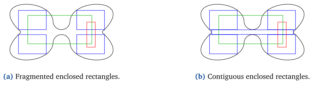
Figure 3. Fragmented versus contiguous enclosed rectangles of polygons.
Some approaches tile the polygon geometry as in the case of a quad-tree, in single- 8 and multi-resolution10 grids respectively. Both approaches use squares to represent the interior of each polygon. As shown in Figure 4 the use of squares might not always be the optimal way to cover the maximal portion of an area. For example, Figure 4a represents the maximal interior area of a polygon with 17 cells, all of them squares of the same size8. Figure 4b represents the same area with 14 cells, all of them squares but with different size10. This figure creates cells of adaptive size, but stays strict to the quad-tree tiling approach. Finally, Figure 4c, which is the one we believe is the most efficient, represents the same area with only five rectangles, that do not have to be squares or have the same size.
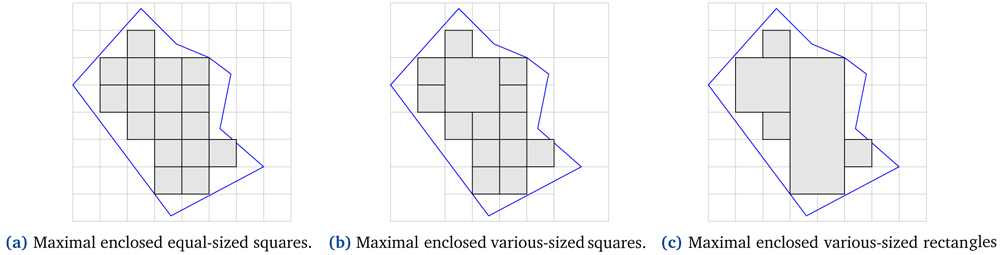
Figure 4. Maximum enclosed squares and rectangles of a polygon.
There are approaches that use a global gridding of the world10 instead of creating a grid for each polygon individually. In the latter case the minimum bounding rectangle of the candidate geometry is used as the gridding domain and the tiling of the geometry is performed as in the case of a quad-tree8. In contrast, the global gridding decides a starting point for the grid,4 and therefore may differ significantly from the grid of more mainstream approaches. In theory, the global gridding does not seem to facilitate the operators between polygons.
As mentioned in the previous section, there are other exterior approximations like minimum bounding rectangles (i.e. rotated minimum bounding rectangles), used during the filtering phase or as an intermediate step before the refinement phase. The approximations can be read from external memory faster than the full object and the intersection tests can be performed faster. Using a better approximation than minimum bounding rectangles generally reduces the number of false hits. However, when calculating the more accurate approximations, the complexity is increased, together with the amount of the storage required (in most cases) and the complexity of the intersection test between the approximated objects4. Therefore, the use of more accurate approximations instead of minimum bounding rectangles can mitigate the benefit.
These interior approximations are illustrated in Figure 5. If the amount of the enclosed rectangles was strictly one, then we would fall into the case described above. The complexity of calculating the more accurate approximations is increased, as well as the complexity of the intersection test between the approximated objects, while the amount of the storage required stays the same. But note that we do not restrict the number of the enclosed rectangles to one. Therefore, the calculating operators (for the approximation and the intersection test) are more expensive for the rotated bounded rectangles (Figure 5a), but the axis-aligned bounded rectangles (Figure 5b) require more storage space in order to cover the same portion of the shape approximating. Consequently, the trade-off between the most economical coverage and the most expensive GIS operators is worth exploring.
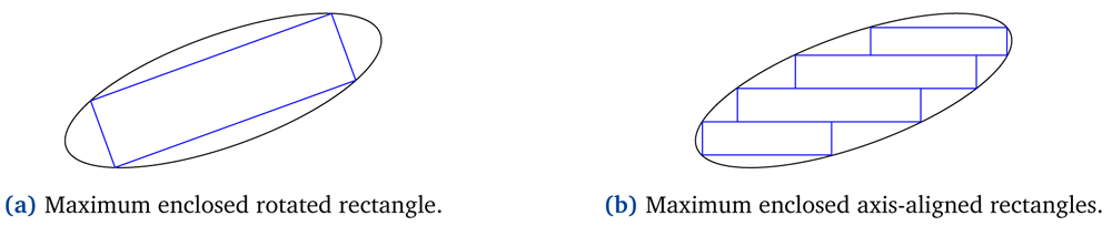
Figure 5. Maximum enclosed rotated and axis-aligned rectangles of a polygon.
In all of the methods mentioned above, it is not equally easy to create a few number of maximal bounded rectangles for all polygons. By few number here, we mean a number of bounded rectangles much fewer than the number of the vertices of the original polygon; what this number could be is something worth investigating. For convex and marginally concave polygons (cf. Figure 1) it is much easier to compute fewer and bigger bounded rectangles in comparison to concave polygons with many reflex interior angles (cf. Figure 3). Simpler polygons (i.e. convex) will produce bounded rectangles that cover a maximal area of the polygon. More complex polygons (i.e. concave) will result in a more significant error rate. That is, the amount of dead space, or the excluded portions of the full object, will be greater. Therefore, the more concave a polygon is, the finer handling it would require. When referring to a more concave polygon we mean that the polygon is not marginally concave; it has many reflex interior angles (cf. Figure 6a). Gridding non-marginally concave polygons into fragmented8,10 is not efficient. The number of rectangles required to cover a large portion of the concave polygon would be significantly large. In such occasions rectangles of various size would be preferable, since it would be easier to cover a greater area with fewer shapes. An algorithm that measures and controls the error rate, or the desired amount of bounded rectangles, would be useful.
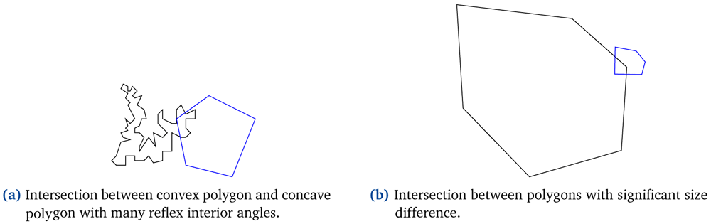
Figure 6.
Intersection examples between a convex polygon and (a) a non-marginally concave polygon, (b) a much larger polygon.
Of particular interest is also the intersection between polygons that have a significant size difference between them, as illustrated in Figure 6b. If both polygons share the same single-resolution grid, it would cost in memory consumption but with no aftermath benefit. In such occasions separate multi-resolution grids that better meet the features of each shape, should be preferred. More concrete, the interior of the shape should be represented by coarse-grained cells and its boundary area by fine-grained cells. Greater polygons should include more coarse-grained cells in their interior, and smaller polygons more fine-grained cells.
Lastly, the decision of whether the bounded rectangles should be entirely within the candidate polygon should be made. For entirely included approximations there will be interior portions of the full object that will be excluded8. On the contrary, for approximations lying at most inside the polygon but allowed to slightly diverge from its boundaries some dead space will be included10. Whether the error rate is minimized in the first or in the second occasion is worth investigating.
Based on the above, we concluded on some rules we believe would be most-efficient for interior approximations in real world scenarios; and on others we believe worth further investigation. The use of a multi-resolution grid for each shape separately results in more accurate approximations. Contiguous interior approximations makes it safe to assume correlations between the containment of vertices of a geometry and the actual containment of the geometry. Also, depending on the complexity of each shape, multiple and intersecting inner rectangles could result in larger coverage. Finally, the decision of whether rotated or axis-aligned inner rectangles is the best choice is not trivial; we will experiment with several shape complexities and sizes later on. In the next section we will present our approach concerning the intermediate step after minimal bounding boxes elimination, before computing precise distances. Initially we intend to deal with simple polygons (i.e. convex and concave), and as a next step include additional rules for managing more complex polygons (i.e. polygons with holes and self-intersecting polygons), especially since they do not make sense as shapes that depict an area on the surface of the earth.
Maximal bounded approximations
In this section we present an approach used to compute the minimum amount of maximal bounded rectangles for a given shape. This algorithm is intended to be used as an intermediate step to filter-and-refine approach to identify candidates that are guaranteed to satisfy a query.
Our approach is as follows. First we decide whether a polygon is convex or concave. Then we create a grid having as gridding domain the minimum bounding rectangle of the polygon and cells that are entirely included in the polygon. Finally we generate the fewest possible maximal rectangles derived from the inner cells of the original polygons. Each of these steps is described below.
Concaveness
We use a classifier to decide whether a polygon is convex or concave. The classifier is based on a well-known algorithm for calculating the interior angles of a polygon13. This algorithm first extracts the boundaries of each geometry, i.e. a line describing the boundary for each polygon. Next it extracts the endpoints for every 2-point line segment for each line. Finally, it creates segments from these points and calculates the azimuth for each smallest angle created from two line segments. This algorithm does not guarantee that the calculated angles are interior angles of the polygon (all angles are have positive values that are below 180°).
In order to calculate the maximum interior angle for each polygon, in order to decide whether it is convex or concave, we altered the final step of the described algorithm (see Extended data14 for the implementation of the altered concaveness classifier). Let us remind, that each one of the angles of a convex polygon is below 180°, while in a concave polygon at least one angle is above 180°. Currently, we only handle simple polygons, as it is not realistic to depict an area on the surface of the earth with intersecting polygons. We also distinguish polygons with holes but discard them, for the time being.
Gridding
Subsequently, we calculate the cells that lie in the interior of each original shape. The gridding is based on an algorithm that creates a different grid for the minimum bounding box of each shape15. The algorithm takes as input the original shape and user-provided granularity for the gridding of the minimum bounding box. For the purposes of our initial experimentation we altered this algorithm to have a fixed granularity and create an axis-aligned grid of each minimum bounding box (see Extended data14 for the implementation of the altered gridding algorithm). Using this algorithm in addition to a query that prunes the external geometries of a shape (see Extended data14 for the implementation of the inner cell selection), we gather the interior cells of the original shape.
Tiling
Finally, we generate the fewest possible maximal rectangles derived from the inner cells of each original polygon. The input of the method we implement is a list of contiguous cells, as can be seen in Sub-figure 7a. The output is a list of all possible maximal rectangle combinations that cover the input area. We implement a recursive algorithm which generates greater rectangles derived from combining the input rectangles either vertically or horizontally. We produce all possible combinations covering the input area and use it as input to the next recursive call of our method, until no new combinations can be derived. More concrete, we propose the naive Algorithm 1 (see Extended data14 for the implementation of the tiling algorithm).
Algorithm 1. Compute all possible maximal rectangle combinations covering the same area as the input rectangles.
Input: a list L of contiguous rectangles.
Output: a list LL of all possible rectangle combinations derived from the input rectangles.
L.removeFirst(A);
CC ← computeCombinations(L);
for each combination C ∈ CC do
for each rectangle R ∈ C do
newCC ← computeCombinations({A, R});
for each combination newC ∈ newCC do
LL.add(newC);
LL.add(C.without(R));
end
end
end
return LL;
In Figure 7 we illustrate the rectangle combinations of four input cells after the first and after the second call of our method. The output list of the third and final call only consists of the last illustrated combination of the second call (cf. red rectangle in Sub-figure 7c).
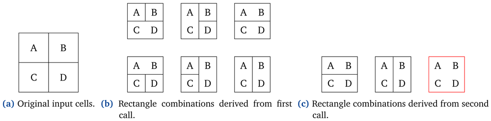
Figure 7. Rectangle combinations during multiple calls of our tiling algorithm.
The final rectangle combinations consist of the fewest possible rectangles with the maximal size, derived from the input rectangles. Emphasis is placed more on the amount of rectangles and their total covering area than on the area covered by each one of them separately. Therefore, the rectangles in the resulting combinations could vary in size, orientation and placement. Figure 8 depicts the maximal rectangle combinations derived from an input of seven cells.
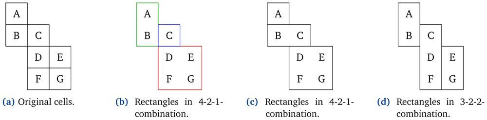
Figure 8. Final maximal rectangle combinations of seven cells.
Note that while generating each combination we ensure that all rectangles included are contiguous. Contiguity implies the existence of a common line segment between two adjacent rectangles; a common point does not suffice to conclude contiguity. According to this convention we observe that the red and the green rectangles in Sub-figure 8b are not contiguous with each other, but are both contiguous with the blue rectangle.5
Finally, we extend the method above to provide maximum coverage for a specific number of rectangles. The rectangles of each combination are sorted based on the amount of the area they cover. The combinations that cover the maximum area using the desired number of rectangles are returned as output. Let us assume a desired number of two maximal rectangles, and the combinations in Figure 8. The first two combinations cover six out of the seven original cells, while the third combination covers only five out of the seven original cells. As a result the third combination would be discarded and the first two would be returned as the possible combinations.
In this section we have presented out Maximal Bounded Approximations approach. That is the computation of the minimum amount of maximal bounded rectangles for a shape, given a grid with cells that are entirely included in it. Let us proceed with its evaluation.
Evaluation
In this section, we use the PostGIS Distance Operator (version 3.1.2) to calculate the distance between shapes of various complexities (i.e. various amount of vertices) and evaluate their performance. Also, we evaluate the performance of our Maximal Bounded Approximations approach. We describe in detail the experimental setup and we analyze the results. The data files (i.e. the full data associated with the experimental evaluation) are available in Underlying data16).
PostGIS distance operator
Experimental Setup. For our first experiment we generate random points, lines and multi-sided polygons17 (see Extended data14 for separate scripts to generate points, lines, polygons and rotated rectangles), 2000 of each, to verify the observation that the number of points of a shape should not significantly affect the time required to calculate its distance from another. Note that the shapes were randomly generated, regardless of whether their MBRs overlap or not.
Experimental results. The notion that calculating the distance between complex polygons is more time consuming than calculating the distance between simpler shapes is correct. Nonetheless, the increase in time is certainly not linear compared to the increase in vertices. In fact, as can be seen from Table 1, calculating distance between 12-sided polygons is about 1.4 times more time consuming (instead of 3) than calculating distance between 4-sided polygons. Between 20-sided polygons is 2 times more time consuming (instead of 5), and between 50-sided polygons 5 more time consuming (instead of 12.5).
Table 1. Experimental results on calculating distance between shapes of various complexity.
The measurements are conducted for calculating the distance from 1000 shapes to 1000 shapes of the same complexity (i.e. from points to points, from lines to lines, etc).
| #points | time (s) | time comparison |
|---|
| points | 1 | 0.93 | |
| lines | 2 | 1.43 | |
| quadrilaterals | 4 | 1.65 | |
| hexagons | 6 | 1.73 | ≈ quadrilaterals |
| dodecagons | 12 | 2.31 | ≈ 1.4 ⋅ quadrilaterals |
| icosagons | 20 | 3.21 | ≈ 2 ⋅ quadrilaterals |
| pentacontagons | 50 | 8.13 | ≈ 5 ⋅ quadrilaterals |
Figure 9 shows the time needed to calculate the distance from various shapes (depicted in the rows i.e. axis-aligned rectangles, rotated rectangles, polygons) to other shapes (depicted in the columns i.e. points, axis-aligned rectangles, rotated rectangles, polygons) (see Extended data14 for the actual numbers used in Figure 9). As expected the distance calculation from any shape to a point is significantly faster, especially as the number of the shapes rises. On contrast, distance calculation between shapes with four or more vertices takes approximately the same amount of time. This comes to intensify the conclusion emerged from Table 1; the number of points of a shape does not significantly affect the time required to calculate its distance from another.
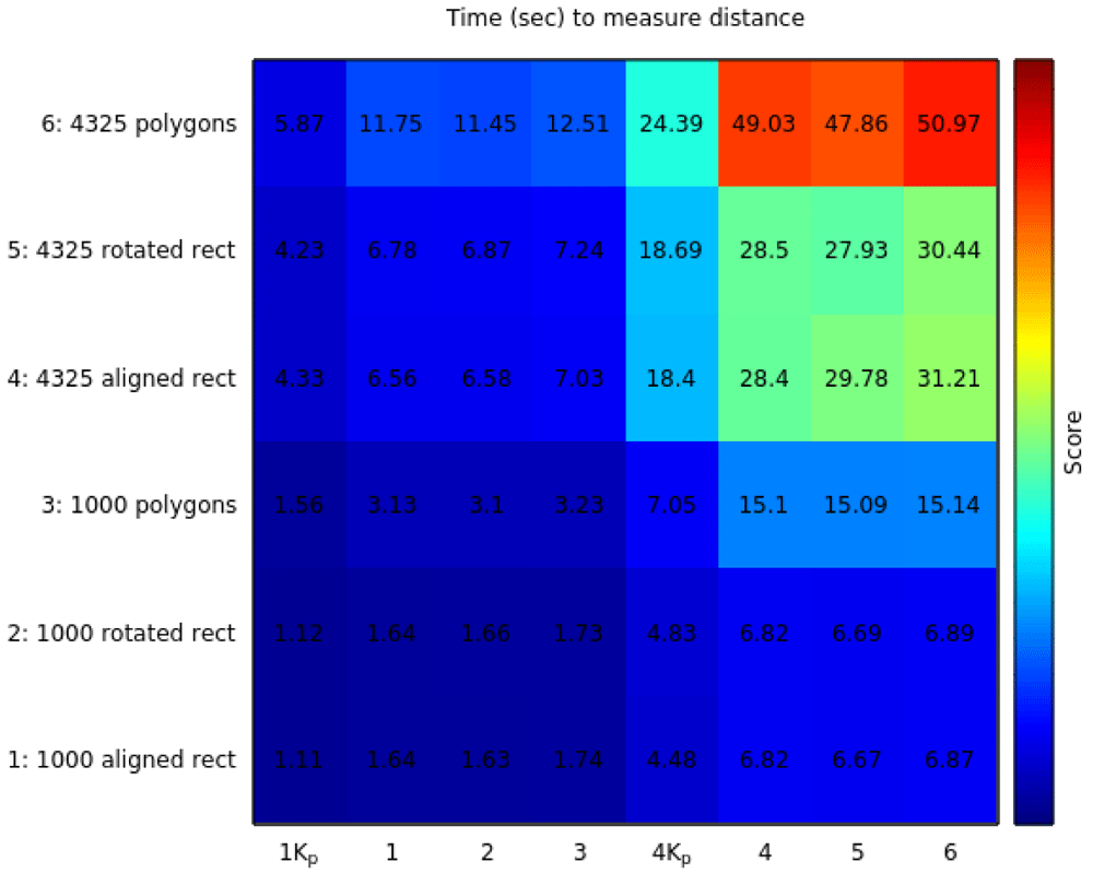
Figure 9. Experimental results on calculating the distance between various number and type of shapes.
The distance is calculated from the shapes in each row to the shapes in each column. 1Kp stands for 1000 points and 4Kp stands for 4325 points.
In the top right corner in Figure 9 we observe that calculating the distance from rectangles to polygons6 is faster than calculating the distance from polygons to rectangles.7
To further investigate this observation we conducted another experiment. We calculated the distance from some rectangles to some polygons, and then from the same polygons to the same rectangles. We shuffled both the rectangles and the polygons and repeated the experiment in the reverse order. We recalculated the distance from the polygons to the rectangles, and then from the same rectangles to the same polygons. The results can be seen in Table 2. Every time, the first run is slower than the second, regardless of which is the source and which the destination in the distance operator. This happens because the results of the first run are probably stored in memory and reused during the second run.
Table 2. Experimental results comparing the ordering of the shapes when distance operation is calculated.
| from | to | run | time |
|---|
| 1000 polygons | 1000 rectangles | 1 | 3.59 sec |
| 1000 rectangles | 1000 polygons | 2 | 2.28 sec |
| 1000 rectangles | 1000 polygons | 1 | 2.56 sec |
| 1000 polygons | 1000 rectangles | 2 | 2.48 sec |
| 4325 polygons | 4325 rectangles | 1 | 2.17 min |
| 4325 rectangles | 4325 polygons | 2 | 1.14 min |
| 4325 rectangles | 4325 polygons | 1 | 3.36 min |
| 4325 polygons | 4325 rectangles | 2 | 1.34 min |
In the following sub-section we evaluate the performance of distance calculation between the original shapes compared to calculating distance between their bounded rectangles.
Maximal bounded approximations
Sources. For the experimental evaluation, we use the following openly available data sources:
The datasets are publicly available as shapefiles. The Invekos dataset contains simple polygons and polygons with holes, while the Lucas dataset contains points. Each dataset is stored in a separate table in a PostGIS database. Table 3 gives more details about these datasets.
Table 3. Dataset statistics.
| dataset | #geospatial data |
|---|
| Invekos | 2,008,137 |
| Lucas | 4,325 |
Queries. The queries that are most relevant for this analysis are within-distance queries; queries retrieving the land parcels with a given crop not within a given minimum distance, without requiring the exact distance. Nevertheless, we use both within-distance and distance queries between polygons and their bounded rectangles and compare the time needed for their calculation.
The queries of the experiment are presented in Table 4. Queries Q1 to Q6 are used for calculating distance from points to geometries, while queries Q7 to Q12 are used for calculating distance from polygons to geometries. Queries Q1 and Q7 are used to compute the distance that equally divides the space of the originating shapes (i.e. points and polygons respectively). The division is conducted separately for each geometry, based on its distance from the originating shapes. That is, for each geometry the 50th percentile of the originating shapes are closer than the calculated distance and the other 50th percentile farther from it. Queries Q2, Q4 and Q8, Q10 use the queries Q1 and Q7, respectively, alongside with the within-distance PostGIS operator to extract shapes (i.e. points and polygons, respectively) that are at-most the given distance away from each geometry. Queries Q3, Q5, Q6 and Q9, Q11, Q12 use the distance PostGIS operator to find the closest shape (i.e. point and polygon, respectively) to each geometry.
Table 4. Queries used in the experiment.
| Queries for points |
|---|
| Q1 | Distance that, for each geometry, equally divides the space that the points lie into. |
| Q2 | Points that are within Q1 distance from each geometry. |
| Q3 | Closest point to each geometry. |
| Q4 | Points that are within Q1 distance from each of the bounded rectangles of each combination of each geometry. |
| Q5 | Closest point to the closest bounded rectangle of each combination of each geometry. |
| Q6 | Closest point to the closest bounded rectangle of the first combination of each geometry. |
| Queries for polygons |
|---|
| Q7 | Distance that, for each geometry, equally divides the space that the polygons lie into. |
| Q8 | Polygons that are within Q7 distance from each geometry. |
| Q9 | Closest polygon to each geometry. |
| Q10 | Bounded rectangles that are within Q7 distance from each of the bounded rectangles of each combination of each geometry. |
| Q11 | Closest bounded rectangle to the closest bounded rectangle of each combination of each geometry. |
| Q12 | Closest bounded rectangle to the closest bounded rectangle of the first combination of each geometry. |
Implementation. We should ensure that the overheads of the bounded rectangles would be recovered from calculating the distance between them; or otherwise their construction would not be appropriate. Let us assume that calculating the distance between two polygons is 10 times slower than calculating the distance between their bounded rectangles. Then, the bounded rectangles should not exceed 10; if they were exactly 10, then calculating the distance between them would result in the same time consumption as in the case of the original polygons. Furthermore, the error rate of the bounded rectangles should be minimal, in order for the grid approximation to cover the maximal possible area of the original polygon. Consequently, according to the results in Table 1, 12-sided polygons should be almost covered by only 1 bounded rectangle, 20-sided polygons from at most 2 bounded rectangles, and 50-sided polygons from at most 5 bounded rectangles; an attempt that would not be realistic, especially for more concave polygons.
During this experimentation we further investigate whether the need of the bounded boxes for a given geometry is directly dependent to their amount. Due to the exhaustive nature of Algorithm 1, the original input cells should not exceed twelve. Otherwise the time to compute the efficient tiling would be significantly long. Also, we arbitrarily set to four the lower limit of the inner rectangles, so that their union would result in changing the input rectangles.
Results. To conduct this experiment we used various numbers of polygons from the Invekos dataset. We first classified them as convex or concave and then calculated the inner cells for each one of them. The original polygons whose inner cells were not contiguous or were more than twelve were discarded (cf. Algorithm 1). Table 5 and Table 6 use the remaining original polygons and their bounded rectangles to answer distance and within-distance queries and measure their time.
Table 5. Experimental results on within-distance (DWithin) and distance (Distance) queries between actual polygons (AP) or their bounded rectangles (BR) and 1000 points.
| (a) Concave shapes |
|---|
| #shapes | measure | DWithin AP | Distance AP | DWithin BR | Distance BR 1st | Distance BR all |
|---|
| 2000 | time (s) | 0.5 | 3.87 | 1.43 | 4.24 | 6.84 |
| rows | 155500 | 311 | 298276 | 311 | 597 |
| 4000 | time (s) | 0.8 | 7.41 | 2.56 | 8.41 | 16.12 |
| rows | 307000 | 614 | 594515 | 614 | 1190 |
| 6000 | time (s) | 1.1 | 11.48 | 4.08 | 12.22 | 27.01 |
| rows | 462500 | 925 | 946731 | 925 | 1895 |
| 8000 | time (s) | 1.3 | 17.11 | 5.08 | 16.79 | 34.5 |
| rows | 602500 | 1205 | 1203564 | 1205 | 2409 |
| 10000 | time (s) | 1.53 | 21.23 | 6.28 | 22.11 | 64.54 |
| rows | 743000 | 1486 | 1500806 | 1486 | 3004 |
| | | | | | |
| (b) Convex shapes |
|---|
| #shapes | measure | DWithin AP | Distance AP | DWithin BR | Distance BR 1st | Distance BR all |
|---|
| 2000 | time (s) | 0.32 | 1.95 | 0.84 | 2.5 | 3.56 |
| rows | 100000 | 200 | 150453 | 200 | 301 |
| 4000 | time (s) | 0.49 | 3.61 | 1.42 | 4.62 | 6.54 |
| rows | 201000 | 402 | 296406 | 402 | 593 |
| 6000 | time (s) | 0.16 | 5.39 | 2.11 | 7.19 | 11.12 |
| rows | 319000 | 638 | 474829 | 638 | 950 |
| 8000 | time (s) | 0.42 | 6.86 | 2.7 | 9.28 | 16.06 |
| rows | 425500 | 851 | 638264 | 851 | 1277 |
| 10000 | time (s) | 0.34 | 8.67 | 3.3 | 12.91 | 20.28 |
| rows | 534500 | 1069 | 796702 | 1069 | 1594 |
Table 6. Experimental results on within-distance (DWithin) and distance (Distance) queries between actual polygons (AP) or their bounded rectangles (BR) and 1000 or 2000 APs or BRs.
| (a) Concave shapes |
|---|
| #shapes | measure | DWithin AP | Distance AP | DWithin BR | Distance BR 1st | Distance BR all |
|---|
| 2K with 1K | time (s) | 0.34 | 0.61 | 0.92 | 0.95 | 1.88 |
| rows | 21459 | 311 | 41147 | 311 | 597 |
| 6K with 1K | time (s) | 0.64 | 1.43 | 2.37 | 2.34 | 5.63 |
| rows | 63825 | 925 | 130580 | 925 | 1895 |
| 10K with 1K | time (s) | 0.92 | 2.26 | 3.57 | 3.62 | 12.87 |
| rows | 102534 | 1486 | 206999 | 1486 | 3004 |
| 10K with 2K | time (s) | 1.64 | 4.82 | 6.82 | 8.64 | 64.95 |
| rows | 200610 | 1486 | 402167 | 1486 | 3004 |
| | | | | | |
| (b) Convex shapes |
|---|
| #shapes | measure | DWithin AP | Distance AP | DWithin BR | Distance BR 1st | Distance BR all |
|---|
| 2K with 1K | time (s) | 0.23 | 0.36 | 0.52 | 0.64 | 0.86 |
| rows | 10800 | 200 | 16242 | 200 | 301 |
| 6K with 1K | time (s) | 0.29 | 0.57 | 1.02 | 1.21 | 2.14 |
| rows | 34452 | 638 | 51239 | 638 | 950 |
| 10K with 1K | time (s) | 0.36 | 0.99 | 1.49 | 1.97 | 3.21 |
| rows | 57726 | 1069 | 85977 | 1069 | 1594 |
| 10K with 2K | time (s) | 0.48 | 1.52 | 2.52 | 3.75 | 6.81 |
| rows | 102624 | 1069 | 152854 | 1069 | 1594 |
For example, let us take the first two rows in Table 6. Following the flow of the experiment, 2000 polygons from the Invekos dataset were classified as convex or concave, and then their bounded rectangles were calculated using their MBRs. For only 311 concave polygons and 200 convex polygons the computed bounded boxes were contiguous and within the twelve range limit. This can be seen in the second row, fourth and sixth column.
Here we are going to explain the values shown in Table 5 and Table 6; the difference between the two tables being that Table 5 gives results when applying distance and within-distance operators between points and polygons; Table 6 gives results when applying distance and within-distance operators between polygons. In both tables, the times for performing the operation using the actual polygons is compared to the times for performing the operation using their bounded-rectangles approximation.
The third and forth columns use as operands the actual polygons, while the last three use their bounded rectangles. The third column shows the results of query Q2; the points that are within a given distance from each polygon. The forth column shows the results of query Q3; the closest point to each polygon. For this query the actual distance calculation is needed. The last three columns show the results of queries Q4, Q5 and Q6.
As can be seen in Table 5, when calculating distance and within-distance from points, all within-distance queries are calculated much faster than all the distance queries. That happens regardless of the second operand; whether the operation is applied between points and polygons or between points and bounded rectangles within-distance queries are calculated much faster. In contrast, in Table 6, that shows the results when the operators are applied on polygons and bounded rectangles, the within-distance queries between the bounded rectangles are slower than distance queries between the actual polygons. In both tables, the fastest computations for each operator are marked in bold on each line depicting time.
These observations are in-line with the discussion on the PostGIS implementation of the distance and within-distance operators (Section Background); and specifically with how only a small number of vertices are actually considered and, subsequently, the computational cost of the distance operator is not linear to the number of vertices. This is even more pronounced for the within-distance operator, where no further calculations are needed when the distance threshold is reached, which is also visible in our results.
Conclusions
In this work we present an approach for constructing the Maximal Bounded Approximation of a shape. Our approach is a recursive algorithm that computes the largest bounded rectangles by combining the rectangles of a first-pass gridding that leaves a minimal dead space between the approximation and the original shape. This work is based on our discussion of the literature, where we see two main lines. On the one hand there is work on optimizing the computation of the within-distance operator between the actual shapes. On the other hand there is work on shape approximations where satisfying the within-distance filter between the approximations guarantees that the filter is also satisfied between the actual shapes. This latter is the line of work that our method extends, motivated by limitations observed in the literature.
Naturally, computing shape approximations comes with an overhead. Any within-distance optimization that uses shape approximations must provide sufficient speedup to recover such overheads. As we initially assumed that the number of points of a shape significantly affects the execution time of the distance operator, we looked for a shape complexity above which our optimization breaks even with its overheads. We experimented with diverse shapes on the distance operator of PostGIS and on our Maximal Bounded Approximations implementation. The results disproved our initial assumption: Due to the optimizations implemented in PostGIS, distance calculation is not cheaper for simpler shapes. Consequently, the overheads of the bounded rectangles would not be recovered from calculating the distance between simpler shapes. The creation and use of maximal bounded rectangles would not lead to faster overall calculation.
GIS is a well-developed and mature field, with few if any opportunities for novel contribution. A promising path could be to investigate how the methods described above can be generalized to three-dimensional data (either 3D-spatial or spatio-temporal). We plan to further investigate the work done on more complex cases; the implementation of the distance operator for 3D shapes and the query optimization for spatio-temporal database systems. As far as we have already seen, emphasis is given on implementing extensions supporting the use of both temporal and spatial queries, while there is not much research done on 3D shapes. As a future work we will research how established relational spatial databases (i.e. PostgreSQL) handle these complex operations, and investigate the limitations of extending the existing approaches for 2D shapes to 3D. This search will provide insights that will guide subsequent steps, and specifically insights about the complexion of the 3D space.
Data availability
Underlying data
For the experimental evaluation, we use the following openly available data sources:
Zenodo: Optimizing Within-Distance Queries by Approximating Shapes with Maximal Bounded Boxes - Datasets. https://doi.org/10.5281/zenodo.574471416.
This project contains the following underlying data, in both csv and sql format:
Figure_9 (Data to calculate the distance between various numbers and types of shapes, i.e. from polygons, rotated and axis aligned rectangles, to points, polygons, rotated and axis aligned rectangles).
Table_1 (Data to calculate the distance between shapes of various complexity, i.e. points, lines, quadrilaterals, hexagons, dodecagons, icosagons, pentacontagons).
Table_2 (Data to compare the ordering of the shapes when distance operation is calculated, (a) from polygons to rectangles, (b) from rectangles to polygons).
Tables_5_6 (Data to calculate within-distance and distance queries between (a) actual polygons, (b) their bounded rectangles, (c) actual polygons and points, (d) their bounded rectangles and points).
Data are available under the terms of Creative Commons Attribution 4.0 International license (CC-BY 4.0).
Ethics and consent
Ethical approval and consent were not required.