Introduction
Due to the important issue of climate change caused by the greenhouse gas effect and to alleviate the decreasing of oil resources, electric vehicles (EVs) and hybrid electric vehicles (HEVs) are being developed more rapidly (Greco, 2016). An EV contains a large number of battery cells and one important issue is to cool the batteries during use. Several cooling methods are in use or being studied and we can classify them into direct cooling, indirect cooling and cooling methods using phase change (Muratori, 2009). In the direct cooling method, a dielectric cooling fluid flows in direct contact to the battery cells. Air-cooling can be used but this is often insufficient (Rao & Wang, 2011), therefore a dielectric fluid like Midel oil is often preferred (Ogata & Hamada, 2001). In the indirect cooling method, the cooling fluid flows into the channels of a cold plate in contact to the batteries (e.g. Bai et al., 2017; Basu et al., 2016; Fan et al., 2019). In the methods using phase change, we can distinguish the methods using a phase change material (Bai et al., 2017; Greco, 2016; Moraga et al., 2016) from the methods using heat pipes (Greco, 2016). A phase change material is a solid material having a melting temperature just above the working temperature of the batteries. If the batteries become too hot, the phase change material begins to melt and the excess of heat cleared by the batteries is absorbed by the phase change material in the form of latent heat of fusion. This method can be used in order to protect the battery against thermal runaway (Xu et al., 2021). Another method uses heat pipes. Heat pipes are a very efficient manner to transport heat from a hot source (the batteries) to a cold source by using a two-phase gas-liquid flow (Zohuri, 2016). In this paper, only indirect cooling by using a cold plate is investigated.
The objective of this paper is to evaluate, by numerical simulations, a battery pack (BP) thermal architecture and thermal management systems (TMS) for an EV. In order to understand the boundary conditions for the new heat exchanger (HE) definition, it is necessary to define the thermal behaviour of the BP. The French Commissariat à l’Energie Atomique et aux Energies Alternatives (hereafter denoted by CEA) and the Spanish society CIDETEC (hereafter denoted by CID) were in charge of developing numerical modelling of a BP and its HE at two different scales: the CFD (computational fluid dynamics) scale which uses very fine meshes and the MOD3 scale which models the BP using a coarser mesh in order to be able to make rapid transient simulations. CID and CEA use the Fluent® (Ansys, USA) software for the CFD modelling activity and the library MOD3 is developed internally in the CEA with the help of Matlab® (The MathWorks Inc, USA) (RRID:SCR_001622) and Simulink®(RRID:SCR_014744). The open source code OpenFoam can also be used to make CFD calculations and Matlab can be replaced by the open source code Python. Two different versions of the HE are tested (the previously existing one and the new A-sample HE) first experimentally and then numerically. The comparison of the simulation’s results to the experimental results allows the simulations to fit different models and to improve their predictions. The new HE has been developed by the Autrichian society MIBA and the experimental measurements campaigns are done by the CEA.
CFD modelling of the battery pack and heat exchanger
The geometry of the BP is very complex and a simplified scheme is illustrated on Figure 1. Therefore, it has been necessary to make some simplifying assumptions in order to numerically model the BP.
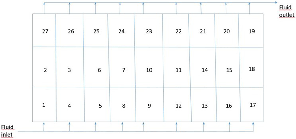
Figure 1. Top view of the battery pack.
The complete BP contains 27 modules (numbered 1-27 in Figure 1), each module containing 12 electrical cells. The modules are separated by aluminium rails which support them. The cells are electrically connected by metallic busbars on the top of them and the HE is placed below the modules. The cold plate (old version of the HE) is constituted of 9 parallel channels, each channel covering three modules hydraulically in series. For example, the 3 modules numbered 17-18-19 on the right side of Figure 1 are hydraulically in series. The nine channels correspond to the nine lines of three modules that are connected hydraulically by two main channels called the liquid distributor and the liquid collector (Figure 2). The coolant fluid inlet and outlet are also indicated on Figure 1. The coolant fluid is a mixture of water and glycol in the proportions of 50% each. A scheme of the cold plate is illustrated on Figure 2.
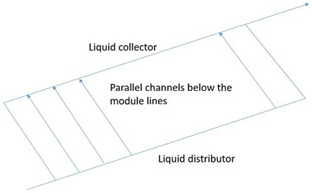
Figure 2. Perspective view of the cold plate (old heat exchanger).
The bottom of the cells in the modules are separated from the channels by a gap-filler (3 mm thick) and one of the objectives of the project was to supress the gap-filler by adopting the new flexcooler technology of MIBA. Three global flow rates of the glycoled water have been included in this study: 0 l/min (no flow rate), 8 and 16 l/min (litres per minute). The heat exchange between the coolant fluid and the internal walls of the channel is quantified by a heat transfer coefficient (HTC expressed in W/m2K: Watt per square meter and per Kelvin) which depends on the distance from each channel inlet. Fine CFD calculations have been done to determine the evolution of this HTC along a channel and the results of these CFD calculations are illustrated on Figure 3. It can be seen that the HTC first decreases from the channel inlet, then tends to an asymptotic value approximately equal to 2000 W/m2K. This kind of evolution is classical (Nellis & Klein, 2012). The decreasing of the HTC is due to the progressive boundary layers thickening. It ceases when the different boundary layers developing along the different walls merge together: the flow becomes thermally established and the HTC becomes constant. The evolution of the HTC obtained by CFD has been mathematically fitted and used in the coarser tool MOD3 (Figure 3).
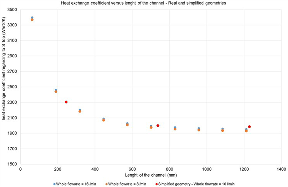
Figure 3. Evolution of the heat exchange coefficient along a fluid channel with different computational fluid dynamic models.
Some CFD simulations have been done at the module level (Figure 4). Each module contains 12 cells represented in the grey colour in Figure 4. The busbars connecting the cells electrically are represented in the blue colour on the figure. This kind of simulation allows the temperature differences between the different cells in the module to be determined (Figure 5). The cell temperature increases along the module since the temperature of the liquid flow below the module regularly increases along its path. Of course, the temperatures of the cells is lower with the greater value of the liquid flow rate.
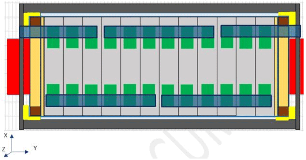
Figure 4. Computational fluid dynamic geometry at the module level.
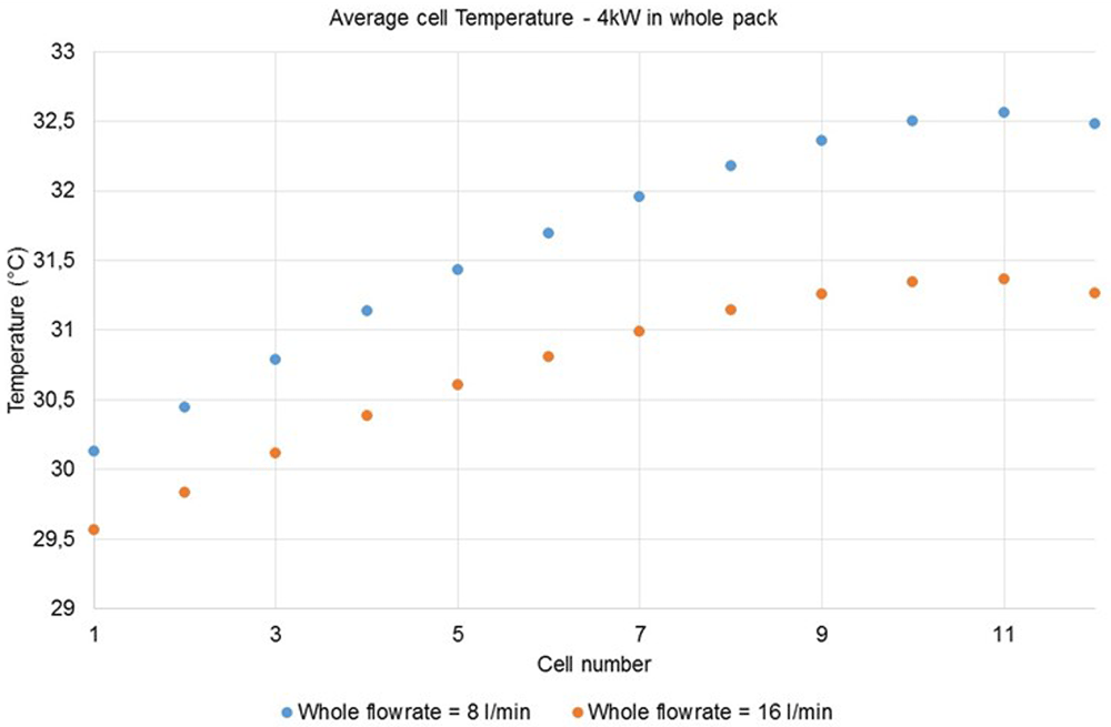
Figure 5. Average temperatures for the 12 cells in the module and for two different liquid flow rates.
The second stage in our CFD developments was to calculate several modules and to take the busbars in-between the modules into account. The geometry modelled with Fluent® for three modules hydraulically in series is illustrated on Figure 6. The Figure 7 shows a view of the corresponding meshing used to realise the simulations. Due to the small dimensions of the busbars and the small thickness of the channels below, a large number of meshes has been necessary for the simulations.
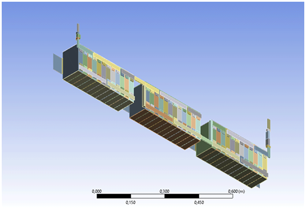
Figure 6. Fluent® geometry model for three modules hydraulically in series.
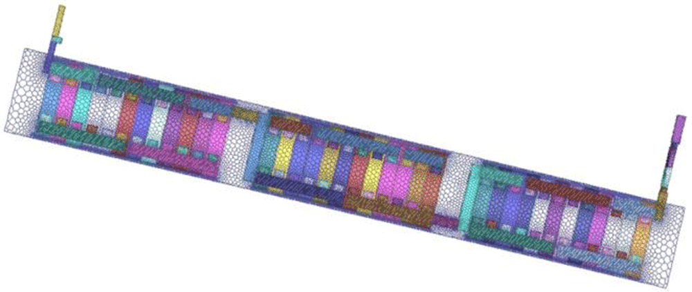
Figure 7. Top view of the meshing.
Both Figure 8 and Figure 9 illustrate the results obtained for a simulation where the power dissipated per cell is equal to 12.34 W and a flow rate value equal to 1.77 l/min (corresponding to a global flow rate equal to 16 l/min since there is nine parallel channels and we simulate only one channel in this simulation). The ambient temperature is assumed to be equal to 23°C and the HTC at the top of the modules is assumed to be equal to 3 W/m2K. It can be seen on the Figure 8 and Figure 9 that the temperature is higher at the top of the cells (since the cooling fluid flows near the bottom of the cells) and that the maximum temperature in each module is obtained at the centre of the module. The temperature increases from one module to the next one. This temperature inhomogeneity between the modules is due to the fluid temperature increasing under the modules since the modules are hydraulically in series.
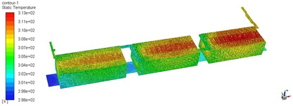
Figure 8. Temperature field (in K) in the three modules and in their underlying water channel.
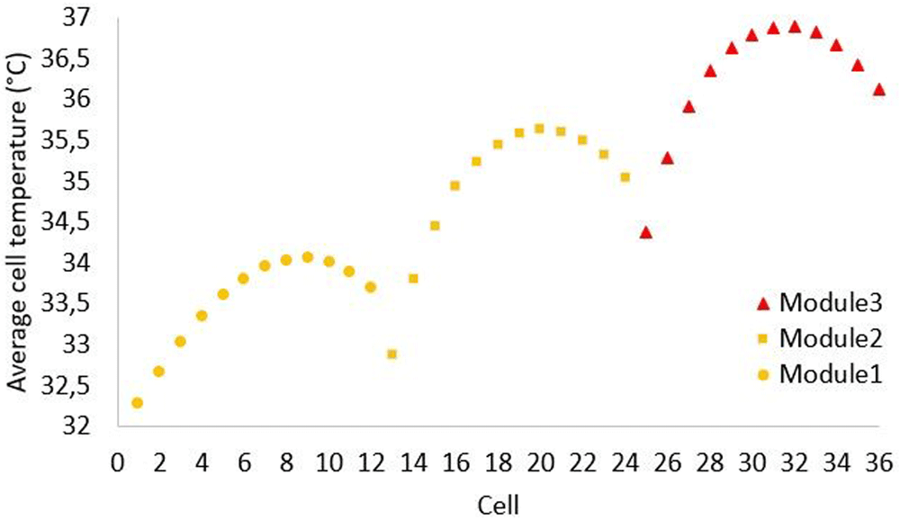
Figure 9. Average cells temperatures (in °C) for the 36 cells in the 3 modules.
The third part of the CFD study tries to model the complete BP for the first time. The thermal behaviour of each element (cells) is related to the efficiency of the HE but also to the thermal bridges generated between the cells and ambient temperature across the BP aluminium rails. Hence, the nearer the module is to the border of the BP, the bigger is the influence of this secondary cooling.
The Figure 10 shows the modelling, in Fluent®, of the real BP which is very complex. The representation of the underlying structure containing essentially the aluminium rails and the casing. Considering the high quantity of cells inside the BP and the computational cost that it could generate, it was determined that implementing only four modules with all 12 cells would be the best compromise. The rest were represented like a uniform block excluding the first and last cells, assuming the importance of these two ones in the thermal behaviour (Figure 11).
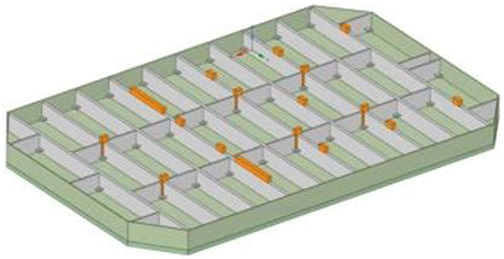
Figure 10. Modelling of the battery pack structure (rails and casing).
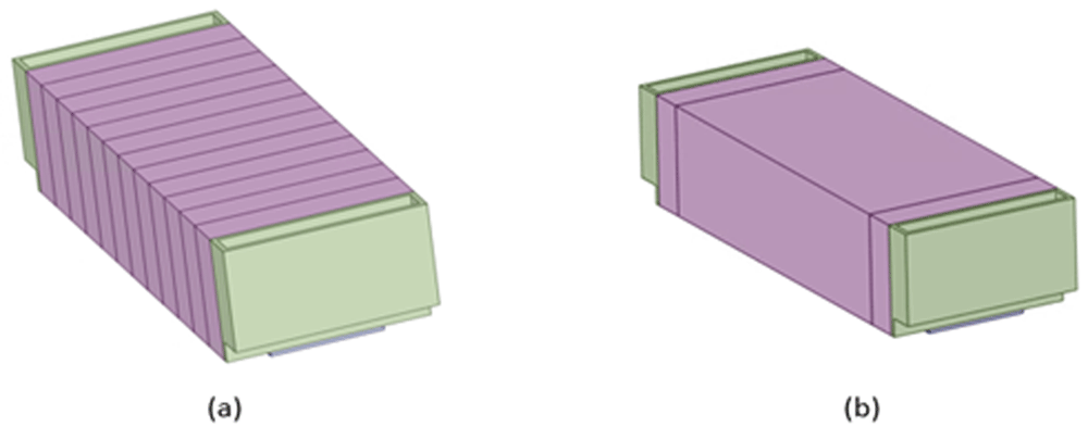
Figure 11.
Model of a real module with 12 cells (a) and a simplified one (b).
The position of the four modules was selected considering the different possible thermal scenarios that could be generated into the BP. The first one was installed in the centre of the BP, where the BP structure’s thermal effect should be minimum. The other three ones were placed forming the last transversal line. This line of modules should characterize the cooling effect of i) BP casing, ii) the HE liquid warmed due to the serial hydraulic design and iii) the test imposed ambient airflow (Figure 12). Air flow was imposed in the climatic chamber (CC) at CEA where the experimental tests were realised.
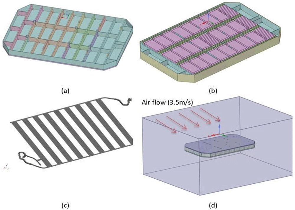
Figure 12.
Modelling of the BP structure (a), the structure including the 27 modules (b) the heat exchanger (c) and the battery pack in the climatic chamber (d).
An excerpt of the meshing used to simulate the complete BP is illustrated on Figure 13. The meshing of the complete BP contains approximately 8 million meshes.
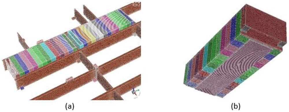
Figure 13.
Views of the meshing of (a) part of the structure with two modules (b) a particular module.
An example of a CFD simulation of the BP casing in the CC with an air flow rate equal to 3.5 m/s is illustrated on Figure 14. It can be seen that the maximum air velocity is attained on the upper face and the lower face of the BP casing. This kind of simulation allows us to determine the HTC between the BP casing and its environment.
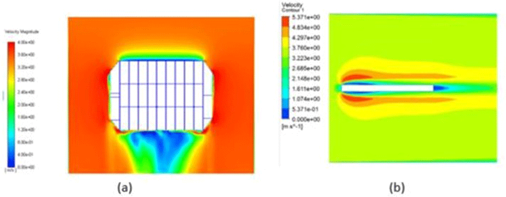
Figure 14.
Simulation of the battery pack in the air flow of the climatic chamber: (a) top view (b) side view.
Another kind of simulation studies the internal thermal behaviour of the BP: transmission of heat between the electrical cells and the aluminium rails and from the rails to the casing and the exterior (Figure 15). It can be seen that the modules in the centre of the BP are hotter than the modules located near its boundaries, showing the cooling by the ambient air (the HE was not used in this simulation).
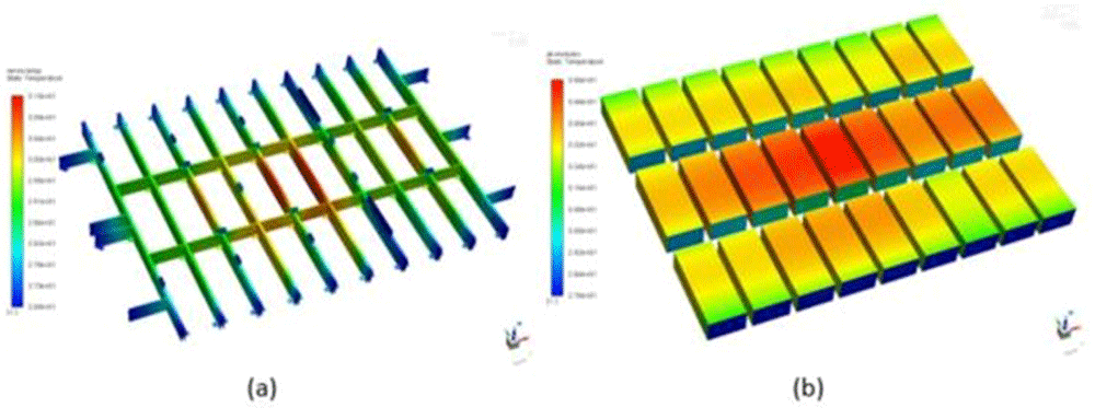
Figure 15.
Temperature fields in (a) the metallic rails (b) the 27 modules.
MOD3 modelling of the complete battery pack and heat exchanger
The CEA develops a numerical program in Matlab+Simulink (called MOD3) able to simulate the thermal behaviour of the BP in transient situations. A similar model could be developed in open source languages like Python or even Fortran. In the previous section, steady CFD simulations were presented. Steady simulations have been preferred in CFD due to the big meshes necessary to do such calculations, implying large computer processing unit (CPU) times (the CPU time is the “cost” of one calculation). In reality, the solicitation of the BP by an electric vehicle is strongly transient in nature, especially in town traffic since the vehicle must change its speed frequently. In our Ihecobatt H2020 European project, a large number of experimental tests have been performed in order to cover different uses of the BP and also to study the performance of the HE in different situations (the HE was the core of the project). Therefore, we need a tool which is able to make a large number of transient simulations, keeping a reasonable CPU time. The MOD3 program is used by CIDETEC in order to tune the TMS of the BP. In order to save CPU time, the meshing of the BP has been considerably reduced in comparison to the grids used in CFD. Typically, a CFD calculation employs several millions of meshes and the meshing in the MOD3 tool employs around 2500 meshes. Due to this strong grid reduction, the MOD3 model has been constructed by means of thermal capacitance and conductance, as will be shown hereafter. A single mesh in MOD3 corresponds to a large number of meshes in the CFD model, therefore a model reduction has been necessary to obtain the MOD3 model. We have only kept some information from the CFD study (HTCs) to build the MOD3 model and its coefficients have been fitted by comparison to the experimental data.
Brief description of the MOD3 model
In this section we describe a numerical method taken from Patankar (1980).
MOD3 is an electro-thermal model coupling the electrical cell model to a three-dimensional thermal model. Here we describe only the thermal part of the MOD3 model. MOD3 is a three-dimensional model defined on a coarse meshing of the BP and the HE. The main equation solved by MOD3 is the following temperature equation:
where ρ is the material density (kg/m3), c is the material heat capacity (J/kgK) and k is the material thermal conductivity (W/mK). s is a possible volumetric source term (W/m3). When the fluid is considered, a convective term is added to the Equation (1). Integrating (1) on the volume of a given mesh, the following equation is obtained:
where V is the mesh volume and ∂V is the bounding surface of the mesh. The first term on the right hand side of (1) has been integrated on the mesh volume then transformed according to the divergence theorem:
The mesh bounding surface is constituted of several plane surfaces Af called faces therefore the integral on ∂V is rewritten as the sum on the mesh faces of the heat diffusive fluxes, each flux being equal to the product of the face conductivity kf, the temperature normal derivative ≝ (∇T.)f and the face area Af.
Denoting P as the centre of the central (current) mesh and F as the centre of one adjacent mesh, f being the face number separating the two meshes P and F, the diffusive flux through face f can be rewritten as:
where TP and TF are the temperatures defined at the cell centres P and F and dPF is the distance between them. Now, looking at Equation (2) and Equation (4), we define:
as the capacitance of a single mesh, m being the mass contained in it. Therefore the capacitance is in Joules per Kelvin (J/K). We also define the conductance through the face f as:
The conductance Hf is expressed in Watts per Kelvin (W/K). The inverse of the conductance is called the thermal resistance:
We can also define the area specific thermal resistance as:
The area specific thermal resistances for a plane wall having a thickness e and a conductivity k and for a convective heat exchange coefficient h are given by:
When two resistances are in series, they must be added, hence we obtain the equivalent resistance and conductance:
When two resistances are in parallel, their conductances must be added, hence we obtain the equivalent resistance and conductance:
All these relations have been used to calculate the capacitance and the conductance characterizing the BP in MOD3 formalism. The discretisation adopted in MOD3 is illustrated on Figure 16, each node representing a mesh centre.
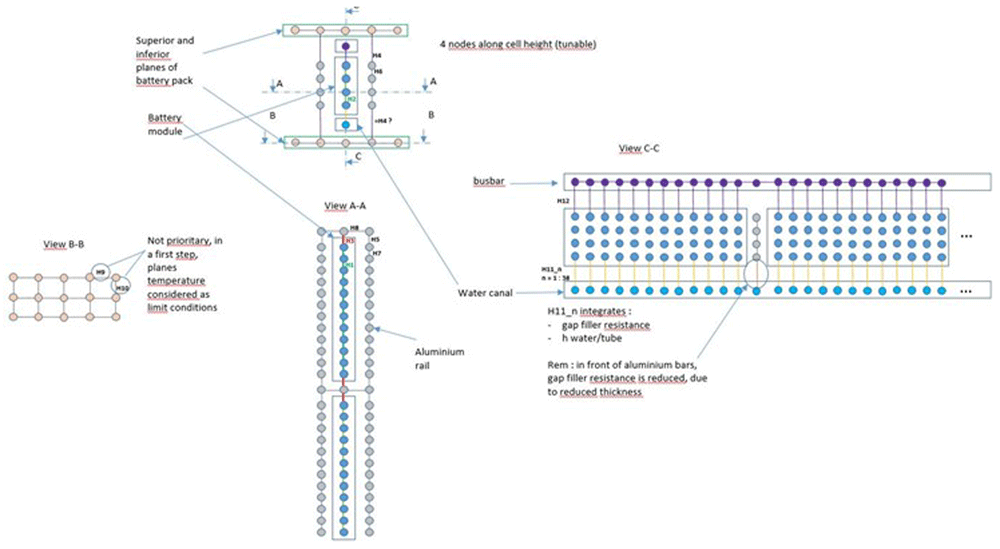
Figure 16. Some sketches of the MOD3 discretisation.
Example of results obtained with the old HE
An important experimental campaign has been done to measure the temperatures with the old (previously existing) HE. This campaign has allowed the study of: the heating and cooling through the air of the CC (in order to determine the HTC between the BP and its surrounding), the heating and cooling through the HE for different values of the liquid flow rate, charge and discharge of the BP at different C-rates (a C-rate equal to 1 corresponds to a complete charge or discharge of the battery in one hour), some pulse tests, some driving cycles on a motorway and heating or cooling by the HE in extreme conditions (ambient temperatures equal to 50°C or -20°C).
All these experimental tests have been calculated with MOD3 and an iterative procedure has been adopted to fit the heat exchange coefficients in the model by comparison to the experiment. Due to the large number of tests and simulations, we will only present a few of them.
The Figure 17 illustrates a comparison between MOD3 results and the experiment for a test of heating in the CC. The initial temperature of the BP is equal to 25°C when it is placed in the CC where the temperature is maintained at 40°C. This kind of test allows qualifying the heat exchange between the BP and its surrounding. This allows us to fit the heat exchange coefficients by natural convection in MOD3. The results obtained for this test were quite accurate when fitting the heat exchange coefficients by natural convection to 10 W/m2K. Figure 17 illustrates the comparison of time evolution of the different temperatures. The continuous lines correspond to the MOD3 results and the dotted lines to the experimental ones. MOD3 is indicated by mod in the legend, followed by the module number and the cell number in each module. T_CM indicates an experimental thermocouple, followed by the module number and the cell number in the module.
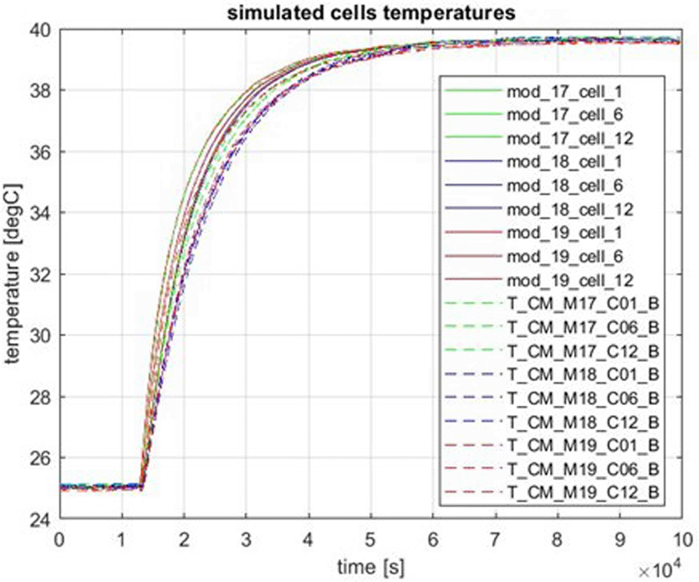
Figure 17. Heating by the air in the climatic chamber.
Figure 18 represents the result obtained for the cooling of the BP by using the HE. The initial temperature of the BP is around 38°C and glycoled water is injected through the HE with an inlet temperature equal to 25°C and a flow rate equal to 16 l/min. Figure 19 gives three liquid temperature curves: the blue curve is the experimental liquid temperature vs time, the red curve is the experimental liquid temperature exiting the HE and the green curve is the liquid temperature at the exit of the HE calculated by MOD3 (the peak at the end of the curve is not physical and should not be considered). It can be seen on these results that MOD3 underestimates the cells temperatures and overestimates the liquid outlet temperature during the first part of the transient. These differences disappear as the BP reaches steady state. This should be due to a too strong heat exchange coefficient between the fluid and the channels (Figure 3) but this is not systematic.
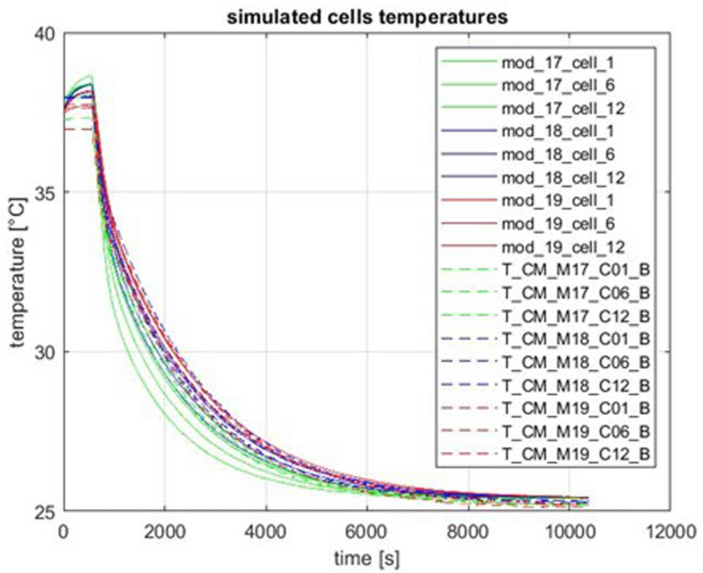
Figure 18. Cooling of the battery pack by using the heat exchanger.
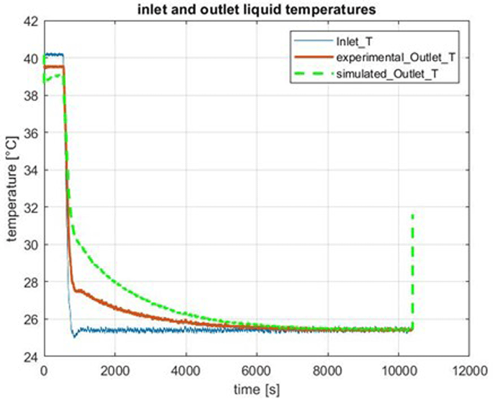
Figure 19. Inlet and outlet liquid temperatures.
Both Figure 20 and Figure 21 show results of several consecutive charges and discharges at 1.5 C-rate cooled by the HE (with a flow rate equal to 16 l/min). Figure 20 corresponds to the modules 17, 18, 19 and the Figure 21 corresponds to the modules 1, 10 and 27 (see Figure 1 for the locations of the modules). The maximum temperatures are slightly underestimated by MOD3.
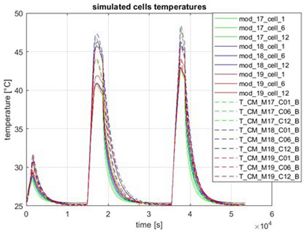
Figure 20. Charge and discharge of the BP at 1.5 C-rate.
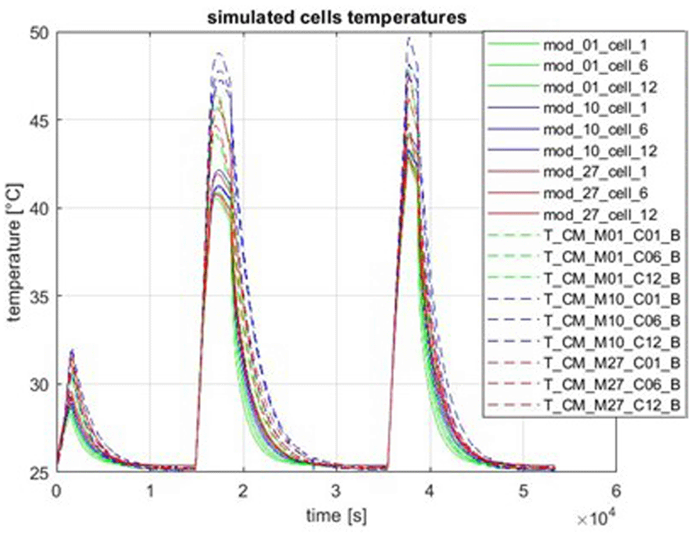
Figure 21. Charge and discharge of the BP at 1.5 C-rate.
The next two figures represent a driving cycle on a motorway (simulated using the CC). Figure 22 illustrates the time evolution of the cells temperatures for the modules 17, 18, 19 and Figure 23 the time evolution of the cooling liquid temperatures at the exit and the inlet.
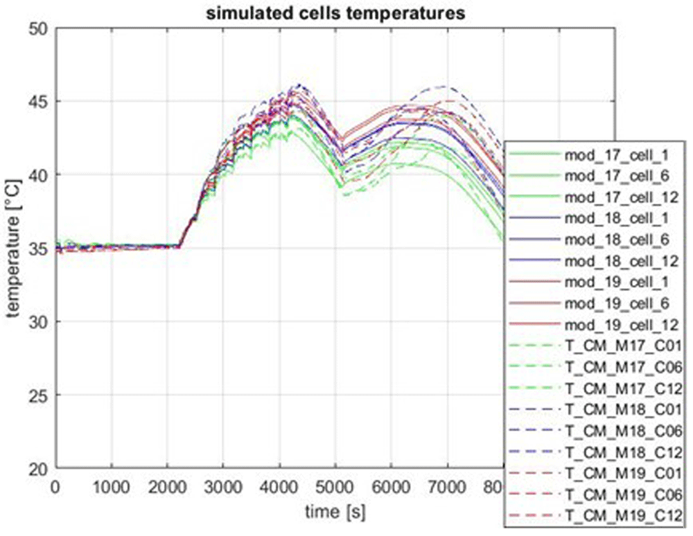
Figure 22. Cells temperature evolution during a driving cycle on a motorway.
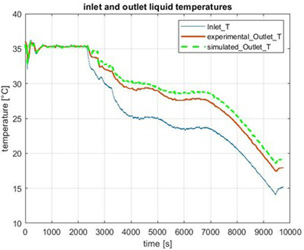
Figure 23. Cooling fluid temperature during a driving cycle on a motorway.
A-sample heat exchanger
Now we will describe the modifications between the old version of the HE and the new one which is called the A-sample. First, the gap-filler in between the battery cells and the liquid channels has been supressed. Second, the channels geometry has been modified (Figure 24). Three different channels with variable cross sections are placed below the nine lines of modules of the complete BP. The grey part on Figure 24 represents a single fluid channel and the white parts the two other channels. Therefore, a single channel covers three consecutive lines of modules and makes two turns around.
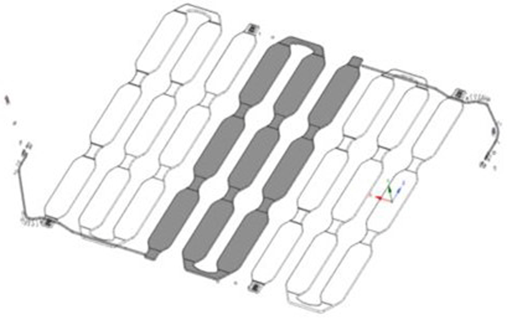
Figure 24. Perspective view of the A-sample heat exchanger.
As there are three different channels, the flow rate inside each channel is equal to the global flow rate divided by three. The horizontal dimensions of one channel are given in Figure 25 and the thicknesses are given in Figure 26.
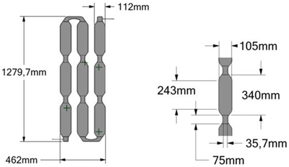
Figure 25. Horizontal dimensions of one channel.
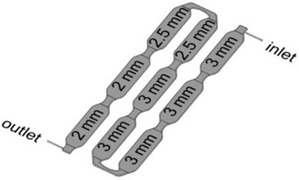
Figure 26. Thicknesses of the channel’s parts.
As the fluid channels have been completely changed, new CFD simulations have been necessary to determine the HTCs between the liquid and the channel walls. One average HTC has been determined from CFD for each MOD3 fluid mesh. There is one such mesh below each electrical cell, therefore we obtain 12 different HTC values for the 12 cells for each module as shown in Figure 27. These values have been implemented in MOD3.
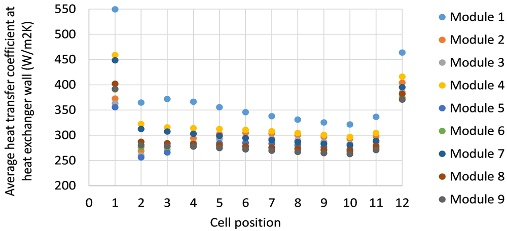
Figure 27. Heat transfer coefficient values in the channels below the nine modules.
Examples of results obtained with the new A-sample HE
The cooling of the BP by the new HE has been studied for different values of the liquid flow rate (8, 12 and 16 l/min). Figure 28 illustrates the cooling of the BP by using the new HE. The global liquid flow rate is equal to 8 l/min and its inlet temperature is equal to 25°C, the initial BP temperature being approximately 38°C. It can be seen that the cells temperatures are slightly overestimated by MOD3.
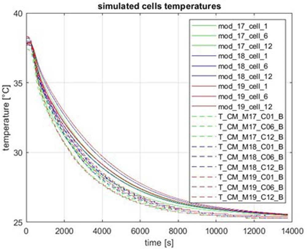
Figure 28. Cooling of the battery pack by the A-sample heat exchanger.
Figure 29 and Figure 30 illustrate a comparison between MOD3 and the measured temperatures for two successive charge and discharge rates with a C-rate equal to 1.5. It can be seen that MOD3 underestimates the temperatures during the two peaks. As can be seen, temperatures were slightly overestimated by MOD3 during the cooling test (Figure 28), it seems that these differences come from an inaccuracy of the electrical cell model rather than the thermal model.
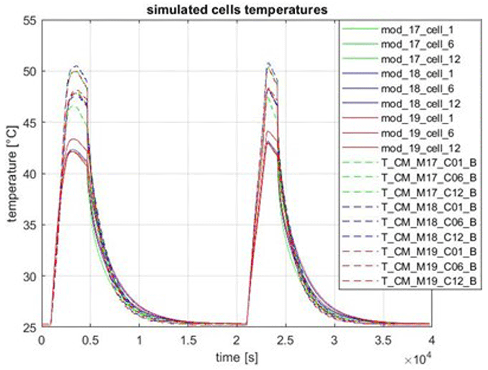
Figure 29. Charge and discharge of the BP at 1.5 C-rate.
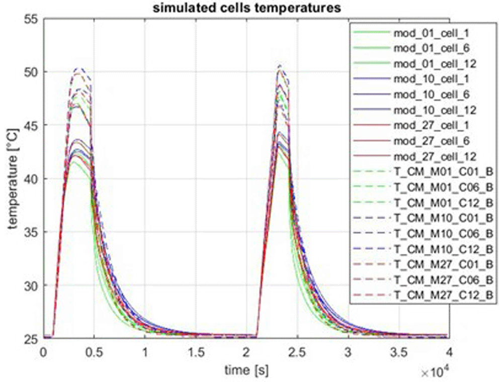
Figure 30. Charge and discharge of the BP at 1.5 C-rate (2).
The next three figures correspond to a driving cycle on a motorway with the new HE. The flow rate was not constant in this test but equal to 16 l/min in a large part of the test and reduced to 8 l/min in the end part of the test, as shown on Figure 31. Figure 32 and Figure 33 show that the temperatures of the cells are slightly underestimated and the temperature of the exiting liquid is slightly overestimated for this test. It seems to show that the HTC are a little bit too high for this test.
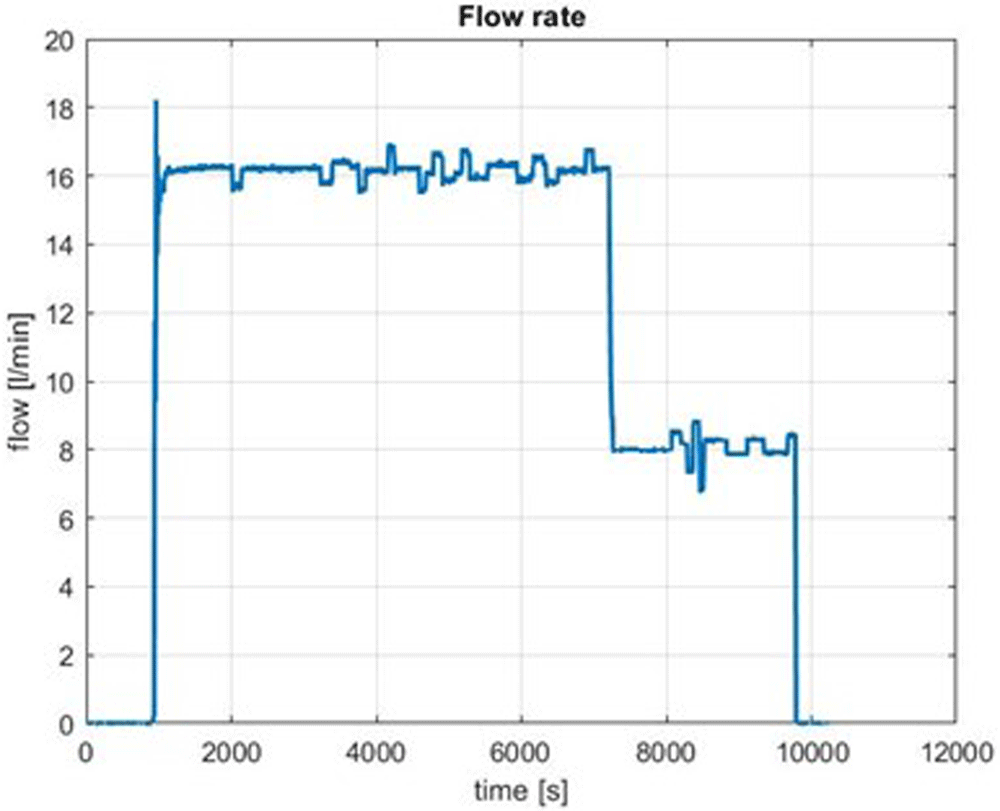
Figure 31. Flow rate evolution during the driving cycle on a motorway.
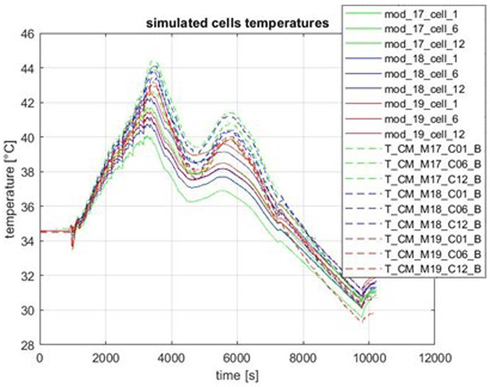
Figure 32. Cells temperature evolution during the driving cycle on a motorway.
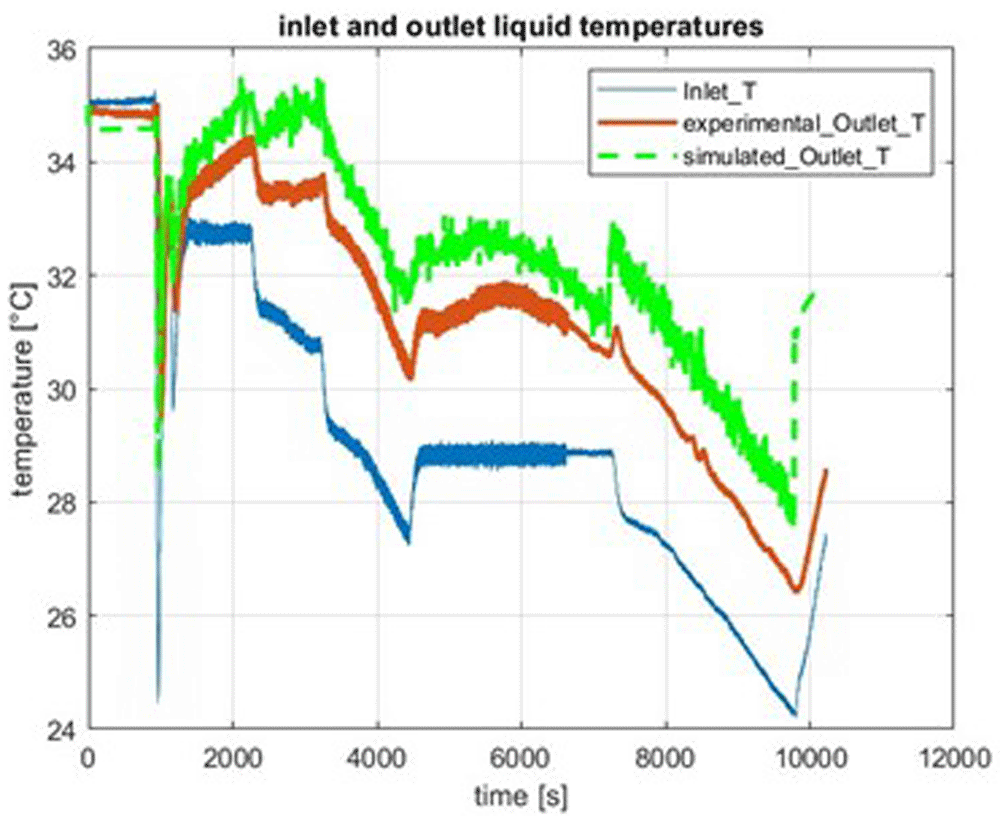
Figure 33. Liquid temperatures during the driving cycle on a motorway.
Conclusions
A thermal modelling of a battery pack (BP) with two versions of a heat exchanger (HE) have been described. The modelling has been done on two different scales, namely the CFD scale which is very fine in terms of spatial discretisation, and the MOD3 scale which is much coarser. Steady CFD simulations allow to obtain heat transfer coefficients which are useful in the MOD3 modelling. MOD3 is a transient computational model which allows long transient simulations like a driving cycle during several hours. The MOD3 results have been compared to the experimental tests completed on the BP at CEA. The next step of this study is the inclusion of MOD3 in the TMS algorithm made at CIDETEC.
Data availability
The data underlying the results cannot be shared for confidentiality reasons. According to the grant agreement signed by all partners and the data management plans, the i-HeCoBatt project follows an Open-Access (OA) approach under the principle "as open as possible, as closed as necessary". However, several of the design and processes developed have the potential for patenting and optimising exploitation. Due to these reasons, the data availability of the defined data sets used to plot the figures is AUDI's property and considered confidential since it has an industrial exploitation objective. In this specific case, to provide access to scientific content to the audience and research data produced, our idea is to prepare an abstract version free of charge to any user for online and open access.
The process of sharing this confidential data starts by contacting the project technical coordinator Mikel Arrinda (marrinda@cidetec.es). The technical coordinator of the project will redirect the data sharing demand to the partner that owns this confidential data. Afterwards, the owner of the data will study the viability of sharing the demanded data on each case based on the consortium IP agreement. The data will only be shared if there are no conflicts of interest and AUDI agrees to the request. If the data is shared, the data receiver will have to fulfil the consortium IP agreement conditions.
Software availability
The software MOD3 used in this work is an in-house development using Matlab/Simulink software. MOD3 has been developed internally and during different projects. MOD3 is not an open-access software. CEA tracks his code changing in a modeling platform called MUSES, using Tuleap environment and a SVN versioning tool. CEA is able to run again with the same version of MOD3 software, the results provided in the paper for the next 10 years.
Ethics and consent
Ethical approval and consent were not required.