This is an outdated version published on August 5, 2022. Read the most recent version.

Improved predictions of phase behaviour of intrinsically disordered proteins by tuning the interaction range

Article

Authors & roles Authors

Peer review record Peer review

Metrics

Cite

Section

Research Article

Published

August 5, 2022

DOI

https://doi.org/10.12688/openreseurope.14967.1

Versions

January 17, 2023 (Version of Record 2.0)
August 5, 2022 (Version of Record 1.0)

European Commission

Grant ID(s): 101025063

Views

1,193

Downloads

343

Citations

See full metrics

intrinsically disordered proteins, liquid–liquid phase separation, force field parameterization, biomolecular condensates, protein interactions

Abstract

The formation and viscoelastic properties of condensates of intrinsically disordered proteins (IDPs) is dictated by amino acid sequence and solution conditions. Because of the involvement of biomolecular condensates in cell physiology and disease, advancing our understanding of the relationship between protein sequence and phase separation (PS) may have important implications in the formulation of new therapeutic hypotheses. Here, we present CALVADOS 2, a coarse-grained model of IDPs that accurately predicts conformational properties and propensities to undergo PS for diverse sequences and solution conditions. In particular, we systematically study the effect of varying the range of the nonionic interactions and use our findings to improve the temperature scale of the model. We further optimize the residue-specific model parameters against experimental data on the conformational properties of 55 proteins, while also leveraging 70 hydrophobicity scales from the literature to avoid overfitting the training data. Extensive testing shows that the model accurately predicts chain compaction and PS propensity for sequences of diverse length and charge patterning, as well as at different temperatures and salt concentrations.

Corresponding author

Giulio Tesei

0000-0003-4339-4460

giulio.tesei@bio.ku.dk

Grant information

This project has received funding from the European Union’s Horizon 2020 research and innovation programme under the Marie Skłodowska-Curie grant agreement No 101025063.

The funders had no role in study design, data collection and analysis, decision to publish, or preparation of the manuscript.

This work is licensed under a Creative Commons Attribution 4.0 International License.

First version published

August 5, 2022 (https://doi.org/10.12688/openreseurope.14967.1)

Latest version published

January 17, 2023 (https://doi.org/10.12688/openreseurope.14967.2)

1 Introduction

Biomolecular condensates may form via phase separation (PS) into coexisting solvent-rich and macromolecule-rich phases. PS is driven by multiple transient interactions which are in many cases engendered by intrinsically disordered proteins (IDPs) and low-complexity domains (LCDs) of multi-domain proteins^1–5. The propensity of IDPs to phase separate and the viscoelastic properties of the condensates are dictated by the amino acid sequence of the constituent IDPs. Moreover, condensates of some IDPs reconstituted in vitro tend to undergo a transition to a dynamically-arrested state, wherein oligomeric species can nucleate and ultimately aggregate into fibrils^2,3,6–14. As accumulating evidence suggests that these processes may be involved in neurodegeneration and cancer^15–18, understanding how PS and rheological properties of condensates depend on protein sequence is a current research focus. Due to the transient nature of the protein-protein interactions underpinning PS, quantitative characterization of biomolecular condensates via biophysical experimental methods is challenging, and hence molecular simulations have played an important role in aiding the interpretation of experimental data on condensates reconstituted in vitro¹⁹. Molecular simulations of the PS of IDPs require a minimal system size of ∼100 chains and long simulation times to sample the equilibrium properties of the two-phase system. Therefore, to enhance computational efficiency, it is useful to reduce the complexity of the system by modeling the solvent as a continuum while coarse-graining the atomistic representation of the protein to fewer interaction sites.

A widely used class of coarse-grained models of IDPs describes each residue as a single site centered at the Cα atom. Charged residues interact via salt-screened electrostatic interactions whereas the remaining nonionic nonbonded interactions are incorporated in a single short-range potential characterized by a set of “stickiness” parameters. The “stickiness” parameters are specific to either the single amino acid or pairs of residues and were originally derived from a hydrophobicity scale²⁰. Other models, based on the lattice simulation engines LaSSI²¹ and PIMMS²², classify the amino acids into a reduced number of residue types with distinct “stickiness”, ranging from binary categorizations into stickers and spacers^4,23,24 to more detailed descriptions and parameterizations^25,26. Recently, the accuracy of the “stickiness” parameters has been considerably improved. This has been achieved by leveraging (i) experimental data on single-chain properties, (ii) statistical analyses of protein structures, and (iii) residue-residue free energy profiles calculated from all-atom simulations^26–31. In particular, we and others have proposed an automated procedure to optimize the “stickiness” parameters so as to maximize the agreement with experimental small-angle X-ray scattering (SAXS) and paramagnetic relaxation enhancement (PRE) NMR data for a large set of IDPs^26,28,29,32. To ensure the transferability of the model across sequence space, we employed a Bayesian regularization approach^32,33. As the regularization term, we defined the prior knowledge on the “stickiness” parameters in terms of 87 hydrophobicity scales reported in the literature. The resulting M1 parameters capture the relative propensities to phase separate of a wide range of IDP sequences. However, we also observed that a systematic increase in simulation temperature of about 30 °C was needed to quantitatively reproduce the experimental concentration of the dilute phase coexisting with the condensate on an absolute scale. Herein, we refer to this model as the first version of the CALVADOS (Coarse-graining Approach to Liquid-liquid phase separation Via an Automated Data-driven Optimisation Scheme) model (CALVADOS 1).

In this class of coarse-grained models of IDPs, nonionic interactions are modeled via a Lennard-Jones-like potential, which decays to zero only at infinite residue-residue distances. For computational efficiency, the potential is typically calculated up to a cutoff distance, r_c, and interactions between particles that are farther apart are ignored. Although this truncation may introduce severe artifacts, in the different implementations of the models, the value of r_c has varied considerably between 1 and 4 nm^{20,29–32,34,35}. Here, we systematically investigate the effect of the cutoff of nonionic interactions on single-chain compaction and PS propensity. We find that decreasing the cutoff from 4 to 2 nm results in a small increase in the radius of gyration whereas the PS propensity significantly decreases. We exploit this effect to improve the temperature-dependence of the CALVADOS 1 model by tuning the cutoff of the nonionic potential. Further, we perform a Bayesian optimization of the “stickiness” parameters using a cutoff of 2.4 nm and an augmented training set. We show that the updated model (CALVADOS 2) has improved predictive accuracy.

2 Methods

2.1 Molecular simulations

Molecular dynamics simulations are conducted in the NVT ensemble using the Langevin integrator with a time step of 10 fs and friction coefficient of 0.01 ps⁻¹. Non-bonded interactions between residues separated by one bond are excluded from the energy calculations. Functional forms and parameters for bonded and nonbonded interactions are reported in the “Bonded and nonbonded interactions” subsection. Single chains of N residues are simulated using HOOMD-blue v2.9.3³⁶ in a cubic box of side length 0.38 × (N − 1) + 4 nm under periodic boundary conditions, starting from the fully extended linear conformation. Each chain is simulated in ten replicas for ∼ 6 × 0.3 × N² ps if N > 100 and for 18 ns otherwise. The initial 100 frames of each replica are discarded, so as to sample 5,000 weakly correlated conformations for each protein (Figure 1). Direct-coexistence simulations are performed using openMM v7.5³⁷ in a cuboidal box of side lengths [L_x, L_y, L_z] = [25, 25, 300], [17, 17, 300] and [15, 15, 150] nm for Tau 2N4R, Ddx4 LCD, and for the remainder of the proteins, respectively. In the starting configuration, 100 chains are aligned along the z-axis and with their middle beads placed in the xy-plane at random (x, y) positions which are more than 0.7 nm apart. Multi-chain simulations are carried out for at least 2 µs, saving frames every 0.5 ns (Figure S1, S2, and S3). After discarding the initial 0.6 µs, the slab is centered in the box at each frame as previously described³² and the equilibrium density profile, ρ(z), is calculated by averaging over the trajectory of the system at equilibrium. The densities of the dilute and protein-rich phases are estimated as the average densities in the regions |z| < z_DS − t/2 and |z| > z_DS + 6t nm, where z_DS and t are the position of the dividing surface and the thickness of the interface, respectively. z_DS and t are obtained by fitting the semi-profiles in z > 0 and z < 0 to ρ(z) = (ρ_a + ρ_b)/2 + (ρ_b − ρ_a)/2 × tanh [(|z| − z_DS )/t], where ρ_a and ρ_b are the densities of the protein-rich and dilute phases, respectively. The uncertainty of the density values is estimated as the standard error obtained from the blocking approach³⁸ implemented in the BLOCKING software (github.com/fpesceKU/BLOCKING).

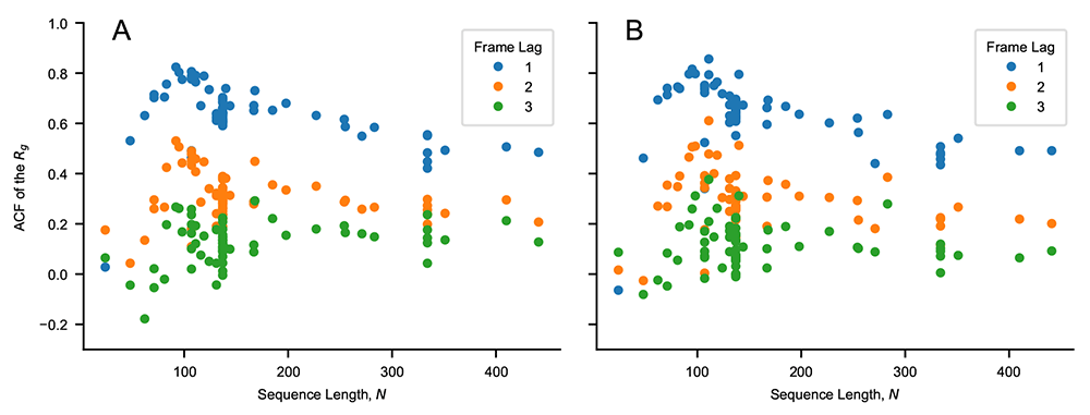
Figure 1. Values of the autocorrelation function of the R_g for a lag time of one, two and three frames as a function of sequence length, N.

The autocorrelation is calculated for the sequences of Table 1 and Table 2 simulated using (A) CALVADOS 1 and (B) CALVADOS 2 for ∼ 6 × 0.3 × N² ps if N > 100 and for 18 ns otherwise. 600 simulation frames are saved every ∼ 0.003 × N² ps if N > 100 and every 30 ps otherwise. The initial 100 frames are discarded from each simulation.

Table 1. Solution conditions and experimental radii of gyration of proteins included in the training set for the Bayesian parameter-learning procedure.

Protein	N	R_g (nm)	T (K)	c_s (M)	pH	Ref.
Hst5	24	1.38 ± 0.05	293	0.15	7.5	45
(Hst5)₂	48	1.87 ± 0.05	298	0.15	7.0	46
p53 (20-70)	62	2.39 ± 0.05	277	0.1	7.0	47
ACTR	71	2.6 ± 0.1	278	0.2	7.4	48
Ash1	81	2.9 ± 0.05	293	0.15	7.5	49,50
CTD2	83	2.61 ± 0.05	293	0.12	7.5	50,51
Sic1	92	3.0 ± 0.4	293	0.2	7.5	52
SH4UD	95	2.7 ± 0.1	293	0.2	8.0	53
ColNT	98	2.8 ± 0.1	277	0.4	7.6	54
p15PAF	111	2.8 ± 0.1	298	0.15	7.0	55
hNL3cyt	119	3.2 ± 0.2	293	0.3	8.5	56
RNaseA	124	3.4 ± 0.1	298	0.15	7.5	57
A1	137	2.76 ± 0.02	298	0.15	7.0	58
-10R	137	2.67 ± 0.01	298	0.15	7.0	58
-6R	137	2.57 ± 0.01	298	0.15	7.0	58
+2R	137	2.62 ± 0.02	298	0.15	7.0	58
+7R	137	2.71 ± 0.01	298	0.15	7.0	58
-3R+3K	137	2.63 ± 0.02	298	0.15	7.0	58
-6R+6K	137	2.79 ± 0.01	298	0.15	7.0	58
-10R+10K	137	2.85 ± 0.01	298	0.15	7.0	58
+12D	137	2.80 ± 0.01	298	0.15	7.0	58
+4D	137	2.72 ± 0.03	298	0.15	7.0	58
+8D	137	2.69 ± 0.01	298	0.15	7.0	58
-9F+3Y	137	2.68 ± 0.01	298	0.15	7.0	58
+12E	137	2.85 ± 0.01	298	0.15	7.0	58
+7K+12D	137	2.92 ± 0.01	298	0.15	7.0	58
+7K+12D blocky	137	2.56 ± 0.01	298	0.15	7.0	58
-4D	137	2.64 ± 0.01	298	0.15	7.0	58
-8F+4Y	137	2.71 ± 0.01	298	0.15	7.0	58
-10F+7R+12D	137	2.86 ± 0.01	298	0.15	7.0	58
+7F-7Y	137	2.72 ± 0.01	298	0.15	7.0	58
-12F+12Y	137	2.60 ± 0.02	298	0.15	7.0	58
-12F+12Y-10R	137	2.61 ± 0.02	298	0.15	7.0	58
-9F+6Y	137	2.65 ± 0.01	298	0.15	7.0	58
αSyn	140	3.55 ± 0.1	293	0.2	7.4	59
FhuA	144	3.34 ± 0.1	298	0.15	7.5	57
K27	167	3.70 ± 0.2	288	0.15	7.4	60
K10	168	4.00 ± 0.1	288	0.15	7.4	60
K25	185	4.10 ± 0.2	288	0.15	7.4	60
K32	198	4.20 ± 0.3	288	0.15	7.4	60
CAHSD	227	4.8 ± 0.2	293	0.07	7.0	61
K23	254	4.9 ± 0.2	288	0.15	7.4	60
Tau35	255	4.7 ± 0.1	298	0.15	7.4	62
CoRNID	271	4.7 ± 0.2	293	0.2	7.5	63
K44	283	5.2 ± 0.2	288	0.15	7.4	60
PNt	334	5.1 ± 0.1	298	0.15	7.5	57,64
PNt Swap1	334	4.9 ± 0.1	298	0.15	7.5	64
PNt Swap4	334	5.3 ± 0.1	298	0.15	7.5	64
PNt Swap5	334	4.9 ± 0.1	298	0.15	7.5	64
PNt Swap6	334	5.3 ± 0.1	298	0.15	7.5	64
GHRICD	351	6.0 ± 0.5	298	0.35	7.3	65,66

Table 2. Solution conditions and experimental radii of gyration of proteins simulated in this study but not included in the training set for the Bayesian parameter-learning procedure.

Protein	N	R_g (nm)	T (K)	c_s (M)	pH	Ref.
DSS1	71	2.5 ± 0.1	288	0.17	7.4	66
p27Cv14	107	2.936 ± 0.13	293	0.095	7.2	67
p27Cv15	107	2.915 ± 0.10	293	0.095	7.2	67
p27Cv31	107	2.81 ± 0.18	293	0.095	7.2	67
p27Cv44	107	2.492 ± 0.13	293	0.095	7.2	67
p27Cv56	107	2.328 ± 0.10	293	0.095	7.2	67
p27Cv78	107	2.211 ± 0.03	293	0.095	7.2	67
PTMA	111	3.7 ± 0.2	288	0.16	7.4	66
NHE6cmdd	116	3.2 ± 0.2	288	0.17	7.4	66
A1 LCD*	131	2.645 ± 0.02	293	0.05	7.5	68
A1 LCD*	131	2.65 ± 0.02	293	0.15	7.5	68
A1 LCD*	131	2.62 ± 0.02	293	0.3	7.5	68
A1 LCD*	131	2.528 ± 0.02	293	0.5	7.5	68
ANAC046	167	3.6 ± 0.3	298	0.14	7.0	66
Tau 2N3R	410	6.3 ± 0.3	298	0.15	7.4	62
Tau 2N4R	441	6.7 ± 0.3	298	0.15	7.4	62

2.2 Bonded and nonbonded interactions

In this study, we used the following truncated and shifted Ashbaugh-Hatch potential³⁹,

u_{A H}^{S P} (r) = {\begin{array}{l} u_{L J} (r) - λ u_{L J} (r_{c}) + 𝜖 (1 - λ), \\ λ [u_{L J} (r) - u_{L J} (r_{c})], \\ 0, \end{array} \begin{array}{l} r \leq 2^{1 / 6} σ \\ 2^{1 / 6} σ < r < r_{c} \\ r > r_{c}, \end{array} (1)

where ϵ = 0.8368 kJ mol⁻¹, r_c = 2 or 4 nm, and u_LJ is the Lennard-Jones potential:

u_{L J} (r) = 4 𝜖 [{(\frac{σ}{r})}^{12} - {(\frac{σ}{r})}^{6}], (2)

σ and λ are arithmetic averages of amino acid specific parameters quantifying size and hydropathy, respectively. For σ, we use the values calculated from van der Waals volumes by Kim and Hummer⁴⁰ whereas, for λ, we use the recently proposed M1 parameters³² and the values optimized in this work.

Salt-screened electrostatic interactions are modeled via the Debye-Hückel potential,

u_{D H} (r) = \frac{q_{i} q_{j} e^{2}}{4 π 𝜖_{0} 𝜖_{r}} \frac{exp (− r / D)}{r} (3)

where q is the average amino acid charge number, e is the elementary charge, $D = \sqrt{1 / (8 π B c_{s})}$ is the Debye length of an electrolyte solution of ionic strength c_s and B(ϵ_r ) is the Bjerrum length. Electrostatic interactions are truncated and shifted at the cutoff distance r_c = 4 nm, irrespective of the value of r_c used for Equation 1. We use the following empirical relationship⁴¹

𝜖_{r} (T) = \frac{5321}{T} + 233.76 - 0.9297 \times T + 1.417 \times 10^{- 3} \times T^{2} - 8.292 \times 10^{- 7} \times T^{3}, (4)

to model the temperature-dependent dielectric constant of the implicit aqueous solution. The Henderson–Hasselbalch equation is used to estimate the average charge of the histidine residues, assuming a pK_a value of 6⁴².

The amino acid beads are connected by harmonic potentials,

u_{b o n d} (r) = \frac{1}{2} k {(r - r_{0})}^{2}, (5)

of force constant k = 8033 kJ mol⁻¹ nm⁻² and equilibrium distance r₀ = 0.38 nm.

2.3 Optimization of the “stickiness” scale

The optimization of the “stickiness” parameters, λ, is carried out to minimize the cost function $ℒ (λ) = 〈 χ_{R_{g}}^{2} (λ) 〉 + η 〈 χ_{P R E}^{2} (λ) 〉 - θ ln [P (λ)]$ using an algorithm which is analogous to the one we previously described³². $χ_{R_{g}}^{2}$ and $χ_{P R E}^{2}$ quantify the discrepancy between model predictions and experimental data, and are defined as $χ_{R_{g}}^{2} = {[(R_{g}^{e x p} - R_{g}^{c a l c}) / σ^{e x p}]}^{2}$ and $χ_{P R E}^{2} = \frac{1}{N_{l a b e l s} N} \sum_{j}^{N_{l a b e l s}} \sum_{i}^{N_{r e s}} {[(Y_{i j}^{e x p} - Y_{i j}^{c a l c}) / σ_{i j}^{e x p}]}^{2}$ , respectively, where σ^exp is the error on the experimental values, Y is either PRE rates or intensity ratios and N_labels is the number of spin-labeled mutants used for the NMR PRE data. In the expression for the cost function, the coefficients are set to η = 0.1 and θ = 0.05. The prior is the distribution of λ, P(λ), derived from a subset of the hydrophobicity scales reported in Table 3 and Table 4 of Simm et al.⁴³. Specifically, only the 70 scales that are unique after min-max normalization (Figure S4) are used for the calculation of P(λ), namely Wimley, BULDG reverse, MANP780101, VHEG790101, JANIN, JANJ790102, WOLR790101, PONP800101–6, Wilson, FAUCH, ENGEL, ROSEM, JACWH, CowanWhittacker, ROSM880101 reverse, ROSM880102 reverse, COWR900101, BLAS910101, CASSI, CIDH920101, CIDH920105, CIDBB, CIDA+, CIDAB, PONG1–3, WILM950101–2, WILM950104, Bishop reverse, NADH010101–7, ZIMJ680101, NOZY710101, JONES, LEVIT, KYTJ820101, SWER830101, SWEET, EISEN, ROSEF, GUYFE, COHEN, NNEIG, MDK0, MDK1, JURD980101, SET1–3, CHOTA, CHOTH, Sweet & Eisenberg, KIDER, ROSEB, Welling reverse, Rao & Argos, GIBRA, and WOLR810101 reverse. P(λ) is obtained via multivariate kernel density estimation, as implemented in scikit-learn⁴⁴, using a Gaussian kernel with bandwidth of 0.05. This prior is 20-dimensional and contains information on the λ-distribution of the single amino acid as well as on the covariance matrix inferred from our selection of 70 hydrophobicity scales (Figure 2).

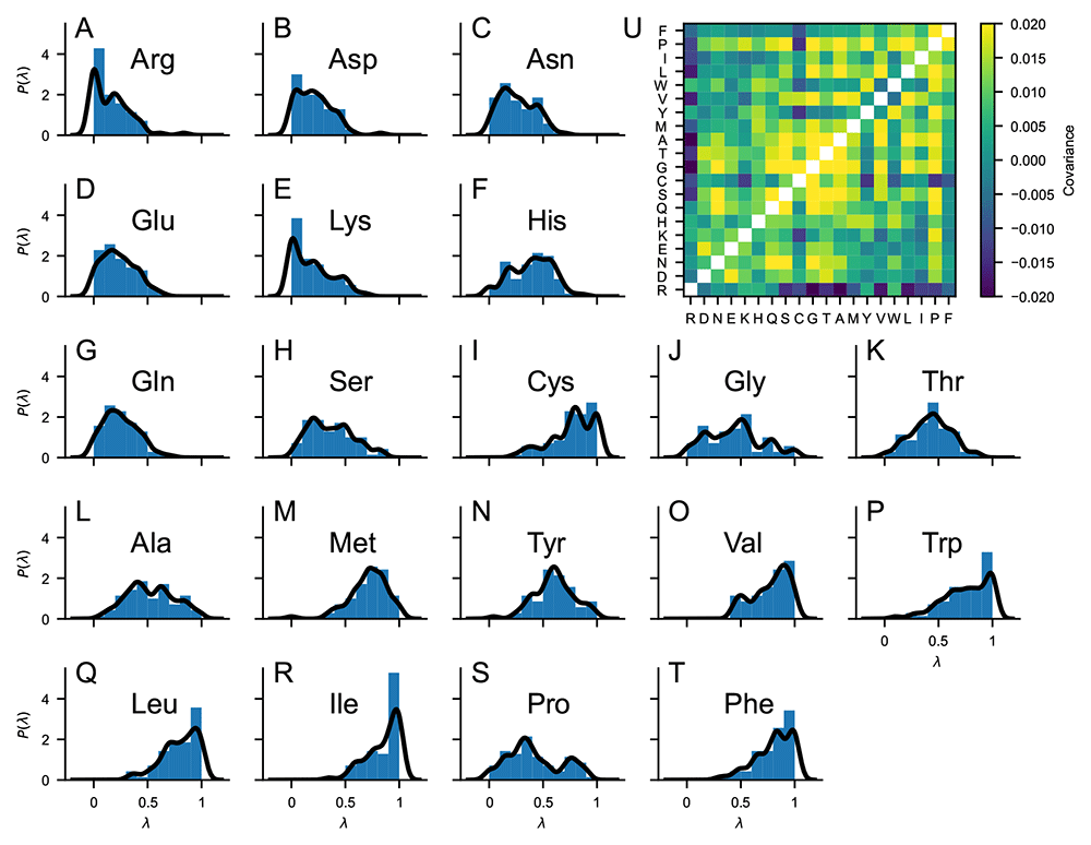
Figure 2.

(A–T) Probability distributions of the “stickiness” parameters, P(λ), obtained from 70 min-max normalized hydrophobicity scales selected from the set by Simm et al.⁴³. Blue bars are histograms with bin width of 0.1. Black lines are obtained as 1D projections of the multivariate kernel density estimation implemented in scikit-learn⁴⁴, using a Gaussian kernel with bandwidth of 0.05. (U) Covariance matrix of the 70 min-max normalized hydrophobicity scales selected from the set by Simm et al.⁴³. The upper triangle of the matrix shows the covariance calculated directly from the 70 min-max normalized hydrophobicity scales whereas the lower triangle of the matrix shows the covariance calculated from the multivariate kernel density estimation averaging over the 70 min-max normalized hydrophobicity scales.

Table 3. Protein and conditions related to the intramolecular PRE data included in the training set.

Protein	N	N_labels	ω_I/2π (MHz)	T (K)	c_s (M)	pH	Ref.
FUS	163	3	850	298	0.15	5.5	2
FUS12E	164	3	850	298	0.15	5.5	2
OPN	220	10	800	298	0.15	6.5	69
αSyn	140	5	700	283	0.2	7.4	70
A2	155	2	850	298	0.005	5.5	3

In the first step of the optimization procedure, the λ values for all the amino acids are set to 0.5, λ₀ = 0.5, and these parameters are used to simulate the proteins of the training set (Table 1 and Table 3). We proceed with the first optimization cycle, wherein, at each k-th iteration, the λ values of a random selection of five amino acids are nudged by random numbers picked from a normal distribution of standard deviation 0.05 to generate a trial λ_k set. For each ith frame, we calculate the Boltzmann weight as w_i = exp {−[U (r_i, λ_k) − U (r_i, λ₀)]/k_BT}, where U is the nonionic potential. The trial λ_k is discarded if the effective fraction of frames, $φ_{e f f} = \exp [- \sum_{i}^{N_{f r a m e s}} w_{i} \log (w_{i} \times N_{f r a m e s})]$ , is lower than 60%. Otherwise, the acceptance probability follows the Metropolis criterion, $\min {1, \exp [\frac{ℒ (λ_{k - 1}) - ℒ (λ_{k})}{ξ_{k}}]}$ , where ξ_k is a unitless control parameter. Each optimization cycle is divided into ten micro-cycles, wherein the control parameter, ξ, is initially set to ξ₀ = 0.1 and scaled down by 1% at each iteration until ξ < 10⁻⁸. From the complete optimization cycle, we select the λ set yielding the lowest estimate of ℒ. Consecutive optimization cycles are performed from simulations runs carried out with the intermediate optimal λ set. To show that the procedure is reproducible and that the final λ set is relatively independent of the initial conditions, we performed an additional optimization procedure starting from the M1 model, λ₀ =M1³². The optimization performed in this work differs from our previous implementation³² also for the following details: (i) nine additional sequences have been included in the training set (Table 1 and Table 3); (ii) single chains are simulated as detailed in the “Molecular simulations” Subsection; (iii) the average radius of gyration is calculated as 〈R_g⟩ instead of $\sqrt{〈 R_{g}^{2} 〉}$ .

3 Results and discussion

When applying a cutoff scheme, we neglect the interactions of residues separated by a distance, r, larger than the cutoff, r_c. For the most strongly interacting residue pair (between two tryptophans), the nonionic potential of the CALVADOS 1 model at r_c = 2 nm takes the value of -5 J mol⁻¹, that is, only a small fraction of the thermal energy (Figure 3A). However, the Lennard-Jones potential falls off slowly whereas the number of interacting partners increases quadratically with increasing r. Therefore, in a simulation of a protein-rich phase, decreasing the cutoff from 4 to 2 nm (Figure 3A) can imply ignoring a total interaction energy per protein of several times the thermal energy. We first look into the effect of the choice of cutoff on the conformational ensembles of isolated proteins. We simulated single IDPs of different sequence length, N = 71–441, and average hydropathy, ⟨λ⟩ = 0.33–0.63. The average radii of gyration, ⟨R_g⟩, calculated from simulation trajectories are systematically larger when we use r_c = 2 nm, compared to the values obtained using r_c = 4 nm. CALVADOS 1 was optimized using the longer r_c and estimating the ensemble average R_g values as the root-mean-square R_g, $\sqrt{〈 R_{g}^{2} 〉}$ . Since $\sqrt{〈 R_{g}^{2} 〉}$ is systematically larger than ⟨R_g⟩, decreasing r_c to 2 nm results in a slight improvement of the agreement between the calculated ⟨R_g⟩ values and the experimental data (Figure 3B).

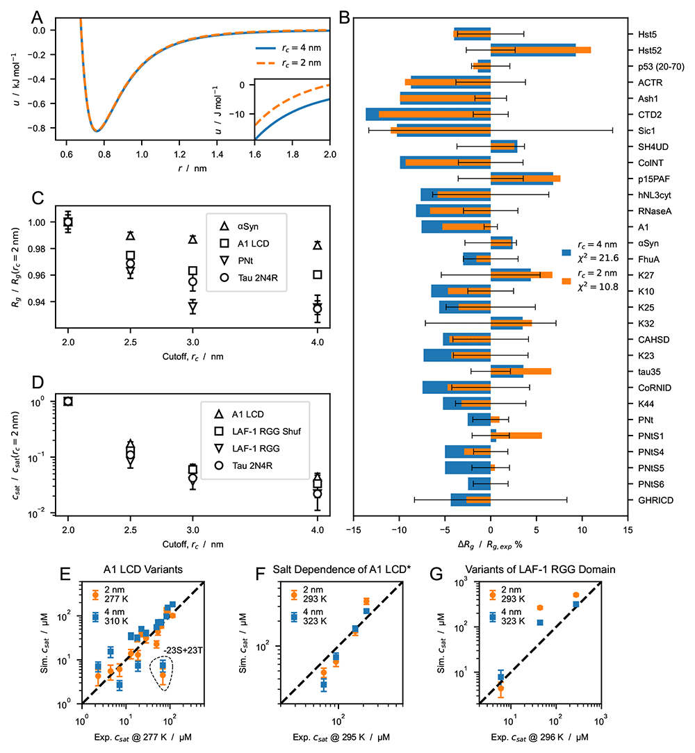
Figure 3. Effect of cutoff size on predictions of radii of gyration, R_g, and saturation concentration, c_sat, from simulations performed using the CALVADOS 1 parameters.

(A) Nonionic Ashbaugh-Hatch potentials between two W residues with cutoff, r_c, of 4 (blue solid line) and 2 nm (orange dashed line). The inset highlights differences between the potentials for r_s ≤ r ≤ r_c. (B) Relative difference between experimental and predicted radii of gyration, ⟨R_g⟩, for r_c = 4 (blue) and 2 nm (orange). $χ_{r}^{2}$ values reported in the legend are calculated for all the sequences in Table 1. (C) ⟨R_g⟩ of α-Synuclein, hnRNPA1 LCD, PNt and human full-length tau (Table 1 and Table 2) from simulations performed with increasing cutoff size, r_c, and normalized by the value at r_c = 2 nm. (D) Saturation concentration, c_sat, for hnRNPA1 LCD, the randomly shuffled sequence of LAF-1 RGG domain, LAF-1 RGG domain and human full-length tau for increasing values of r_c and normalized by the c_sat at r_c = 2 nm. (E–G) Correlation between c_sat from simulations and experiments for (E) A1 LCD variants, (F) A1 LCD∗ WT at [NaCl] = 0.15, 0.2, 0.3 and 0.5 M and (G) variants of LAF-1 RGG domain (Table 4).

To gain further insight into the effect of the cutoff, we performed simulations of single chains of α-Synuclein, hn-RNPA1 LCD, PNt and Tau 2N4R (Table 1 and Table 2) using r_c = 2, 2.5, 3 and 4 nm. Irrespective of the sequence, ⟨R_g⟩ decreases monotonically with increasing r_c. However, the effect on compaction appears to be larger for long sequences and high content of hydrophobic residues, both of which result in an increased number of shorter intramolecular distances. For example, upon increasing the r_c from 2 to 4 nm, the ⟨R_g⟩ of α-Synuclein (N = 140, ⟨λ⟩ = 0.33) decreases by 2.3% whereas the effect is more pronounced for hnRNPA1 LCD (N = 137, ⟨λ⟩ = 0.61) and Tau 2N4R (N = 441, ⟨λ⟩ = 0.38), with a decrease in ⟨R_g⟩ of 4.0% and 7.7%, respectively.

To investigate the effect of the cutoff distance on PS propensity, we performed direct-coexistence simulations of 100 chains of hnRNPA1 LCD, LAF-1 RGG domain (WT and shuffled sequence with higher charge segregation), and Tau 2N4R (Table 4). From the simulation trajectories of the two-phase system at equilibrium, we calculate c_sat, i.e. the protein concentration in the dilute phase coexisting with the condensate. The higher the c_sat value, the lower the propensity of the IDP to undergo PS. As expected from the increased contact density in the condensed phase, the choice of cutoff has a considerably larger impact on c_sat than on chain compaction: decreasing r_c from 4 to 2 nm results in an increase in c_sat of over one order of magnitude. In contrast to what we observed for the ⟨R_g⟩, the decrease in c_sat does not show a clear dependence on sequence length and average hydropathy.

Table 4. Proteins and conditions used for the direct-coexistence simulations performed in this study and references to the experimental data.

Shaded rows highlight systems which are not included in the correlation plot of Figure 7C.

Protein	N	c_s (mM)	pH	Ref.	T (K)
Protein	N	c_s (mM)	pH	Ref.	4 nm	2 nm	Figure 3D
6His-TEV-Lge1₁₋₈₀-StrepII WT	114	100	7.5	71	-	293	-
6His-TEV-Lge1₁₋₈₀-StrepII -11R+11K	114	100	7.5	71	-	293	-
6His-TEV-Lge1₁₋₈₀-StrepII -14Y+14A	114	100	7.5	71	-	293	-
A1 LCD WT	137	150	7.0	4, 58	310 & 323	277 & 293	310
A1 LCD +7F-7Y	137	150	7.0	58	310 & 323	277 & 293	-
A1 LCD -12F+12Y	137	150	7.0	58	310 & 323	277 & 293	-
A1 LCD -23S+23T	137	150	7.0	58	310 & 323	277 & 293	-
A1 LCD -14N+14Q	137	150	7.0	58	310 & 323	277 & 293	-
A1 LCD -10G+10S	137	150	7.0	58	310 & 323	277 & 293	-
A1 LCD -20G+20S	137	150	7.0	58	310 & 323	277 & 293	-
A1 LCD -30G+30S	137	150	7.0	58	323	293	-
A1 LCD +23G-23S	137	150	7.0	58	323	293	-
A1 LCD +23G-23S+7F-7Y	137	150	7.0	58	323	293	-
A1 LCD +23G-23S-12F+12Y	137	150	7.0	58	323	293	-
A1 LCD -9F+3Y	137	150	7.0	58	310	277	-
A1 LCD -8F+4Y	137	150	7.0	58	310	277	-
A1 LCD -3R+3K	137	150	7.0	58	310	277	-
A1 LCD -6R	137	150	7.0	58	310	277	-
A1 LCD -4D	137	150	7.0	58	310	277	-
A1 LCD +4D	137	150	7.0	58	310	277	-
A1 LCD +8D	137	150	7.0	58	310	277	-
A1 LCD +2R	137	150	7.0	58	310	277	-
A1 LCD* WT	131	150	7.0	72	323	293	-
A1 LCD* WT	131	200	7.0	72	323	293	-
A1 LCD* WT	131	300	7.0	72	323	293	-
A1 LCD* WT	131	500	7.0	72	323	293	-
LAF-1 RGG Domain	176	150	7.5	73	323	293	293
LAF-1 RGG Domain Shuffled	176	150	7.5	73	323	293	323
LAF-1 RGG Domain ∆21-30	166	150	7.5	73	323	293	-
A2 LCD	155	10	5.5	74	-	297	-
FUS LCD	163	150	7.4	75	-	297	-
Ddx4 LCD	236	130	6.5	76	-	297	-
Human Full-Length Tau (2N4R)	441	70	7.4	-	-	-	277

From the multi-chain trajectories of hnRNPA1 LCD, LAF-1 RGG domain (WT and shuffled sequence) and Tau 2N4R obtained using r_c = 4 nm, we estimate that the increase in nonionic energy per protein upon decreasing the cutoff from 4 to 2 nm is 13±1 kJ mol⁻¹ (mean±standard deviation), respectively (Figure 4A). Assuming that the number of interactions neglected by the shorter cutoff is proportional to the sequence length and the amino acid concentration in the condensate, the small variance in the energy increase across the different IDPs finds explanation in the fact that the simulated systems display similar values of N² × c_con (Figure 4A), where c_con is the protein concentration in the condensate. The ratio U (r_c = 2 nm)/U (r_c = 4 nm) of the nonionic energies for r_c = 2 and 4 nm is also largely system independent (Figure 4B). Moreover, decreasing the temperature by ∼30 K in the range between 310 and 323 K has a rather small impact on the relative strength of the electrostatic interactions with respect to the thermal energy, due to the decrease in the dielectric constant of water with increasing temperature (Figure 4C). Therefore, we speculate that the effect of decreasing r_c can be compensated by simulating the system at a lower temperature (Figure 4B).

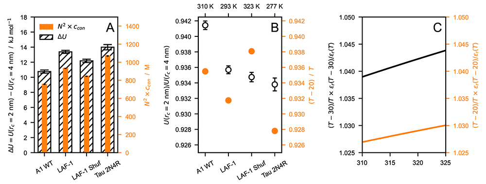
Figure 4.

(A) Comparison between nonionic energy difference per protein (∆U = U (r_c = 2 nm) − U (r_c = 4 nm), hatched) and N² × c_con (orange), where N is the sequence length and c_con is the molar protein concentration in the condensate. (B) Ratio between nonionic energies calculated with r_c = 2 and 4 nm (open circles) compared to the ratio of the thermal energy at T′ = T − 20 K and at T (orange). (C) Increase in electrostatic energy relative to the thermal energy upon decreasing the temperature by 30 (black) and 20 K (orange). The data shown in this figure are obtained from simulations of hnRNPA1 LCD, LAF-1 RGG domain (WT and shuffled sequence) and Tau 2N4R performed at T = 310, 293, 323, and 277 K, respectively, and using r_c = 4 nm. Error bars are standard deviations over trajectories of the systems at equilibrium.

With these considerations in mind, we use the CALVADOS 1 model with r_c = 2 nm to run direct-coexistence simulations of IDPs for which c_sat has been measured experimentally (Table 4), i.e. variants of hnRNPA1 LCD, hnRNPA1 LCD* at various salt concentrations, and LAF-1 RGG domain variants. As we have shown that decreasing the range of the nonionic interactions disfavours PS, we perform these simulations at the experimental temperatures, which are lower by ∼30 K than those required to reproduce the experimental c_sat values when the model is simulated with r_c = 4 nm (Figure 3E–G). The two-fold decrease in r_c enables the model to quantitatively recapitulate the experimental c_sat data at the temperature at which the experiments were conducted. Notably, we show this for diverse sequences, across a wide range of ionic strengths, and for variants with different charge patterning and numbers of aromatic and charged residues. These results suggest that the range of interaction of the Lennard-Jones potential may be too large⁷⁷. While the r⁻⁶ dependence is strictly correct for dispersion interactions between atoms, the nonionic potential of our model incorporates a variety of effective nonbonded interactions between residues, and hence the Lennard-Jones potential is not expected to capture the correct interaction range³¹.

Since CALVADOS 1 was developed using r_c = 4 nm, we examined whether reoptimizing the model with the shorter cutoff could result in a comparably accurate model. As detailed in the Methods Section, we performed a Bayesian parameter-learning procedure³² using an improved algorithm, an expanded training set (Table 1), and r_c = 2 nm. Figure S5 shows that the new model tends to underestimate the c_sat values of the most PS-prone sequences. We hypothesize that during the optimization the reduction of attractive forces due to the shorter cutoff is overcompensated by an overall increase in λ. We tested this hypothesis by performing the optimization with increasing values of r_c, in the range between 2.0 and 2.5 nm, and found that the c_sat values predicted from simulations performed with r_c = 2.0 nm tend to increase with the r_c used for the optimization (Figure 5).

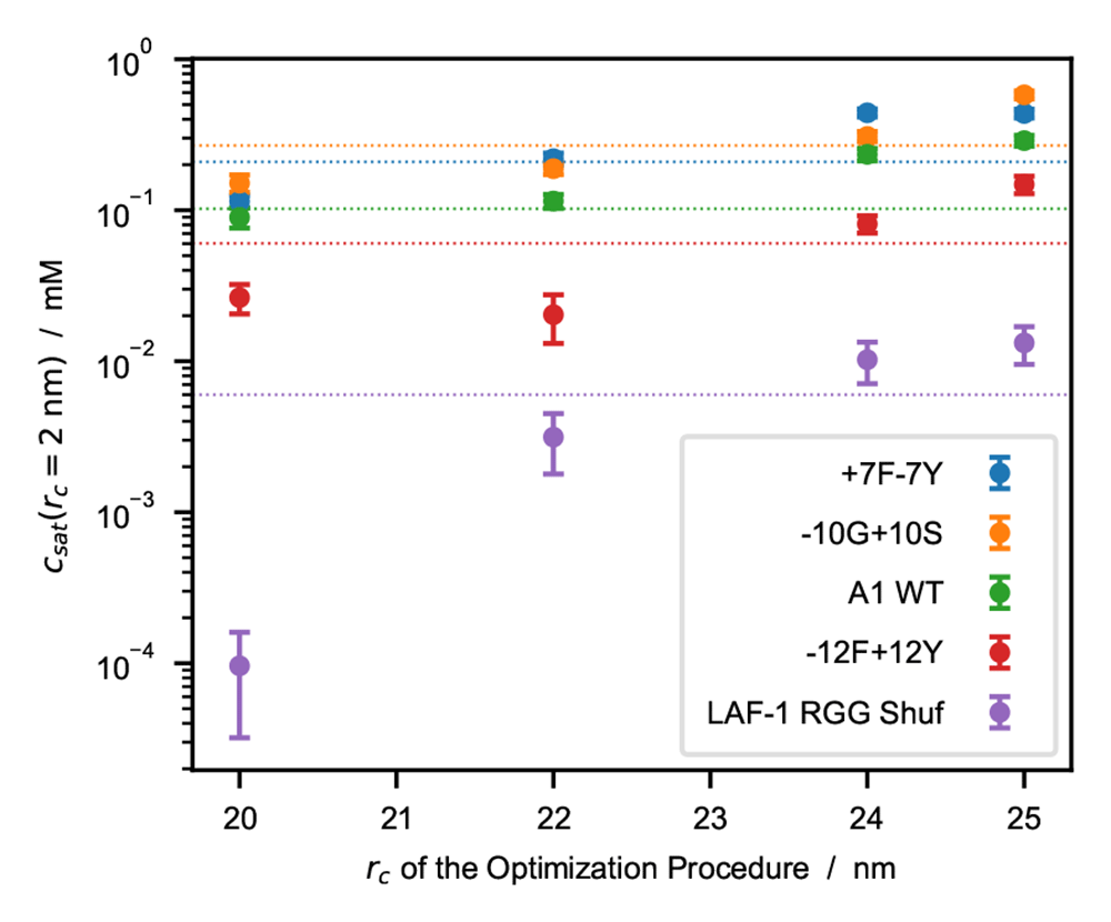
Figure 5. Saturation concentrations, c_sat, as a function of the cutoff used to optimize the model.

c_sat values are calculated from simulations performed using r_c = 2.0 nm whereas the models are optimized using r_c = 2.0, 2.2, 2.4, and 2.5 nm. Horizontal dotted lines represent experimental c_sat values from the references reported in Table 4.

Using r_c = 2.4 nm for the optimization resulted in a model with improved accuracy compared to CALVADOS 1 (Figure 6), especially for the PS of LAF-1 RGG domain and the −23S+23T variant of A1 LCD. To test the robustness of the approach, the optimization was carried out starting from λ₀ = 0.5 for all the amino acids (Figure 6) and from λ₀ =M1 (Figure S6 and S7). The difference between the resulting sets of optimal λ values (Figure S7A) is lower than 0.08 for all the residues and exceeds 0.05 only for S, T and A. The model obtained starting from λ₀ = 0.5 is more accurate at predicting PS propensities and will be referred to as CALVADOS 2 hereafter.

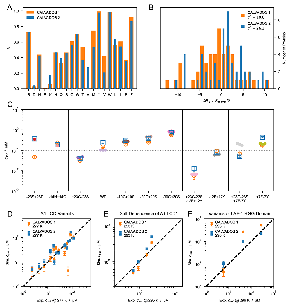
Figure 6.

(A) Comparison between λ sets of CALVADOS 1 (orange) and CALVADOS 2 (blue). (B) Distribution of the relative difference between experimental (Table 1) and predicted radii of gyration, ⟨R_g⟩, for CALVADOS 1 (orange) and CALVADOS 2 (blue). (C) Comparison between saturation concentrations, c_sat, at 293 K of variants of hnRNPA1 LCD measured by Bremer, Farag, Borcherds et al.⁵⁸ (closed circles) and corresponding predictions of CALVADOS 1 (open orange circles) and CALVADOS 2 (open blue squares). (D–F) Correlation between c_sat from simulations and experiments for (D) A1 LCD variants, (E) A1 LCD∗ WT at [NaCl] = 0.15, 0.2, 0.3 and 0.5 M and (F) variants of LAF-1 RGG domain (Table 4).

The λ values of CALVADOS 1 and 2 differ mostly for K, T, A, M, and V, whereas the smaller deviations (|∆λ| < 0.09) observed for Q, L, I, and F (Figure 6A) are within the range of reproducibility of the method (Figure S7A). Although CALVADOS 1 was optimized using r_c = 4 nm, predictions of single-chain compaction from simulations performed using r_c = 2 nm are more accurate for CALVADOS 1 than for CALVADOS 2. This result can be explained by the opposing effects of decreasing the cutoff and calculating R_g values as ⟨Rg⟩ instead of $\sqrt{〈 R_{g}^{2} 〉}$ . In fact, the $\sqrt{〈 R_{g}^{2} 〉}$ values predicted by CALVADOS 1 are strikingly similar to the ⟨R_g⟩ values predicted by CALVADOS 2 (Figure 7A).

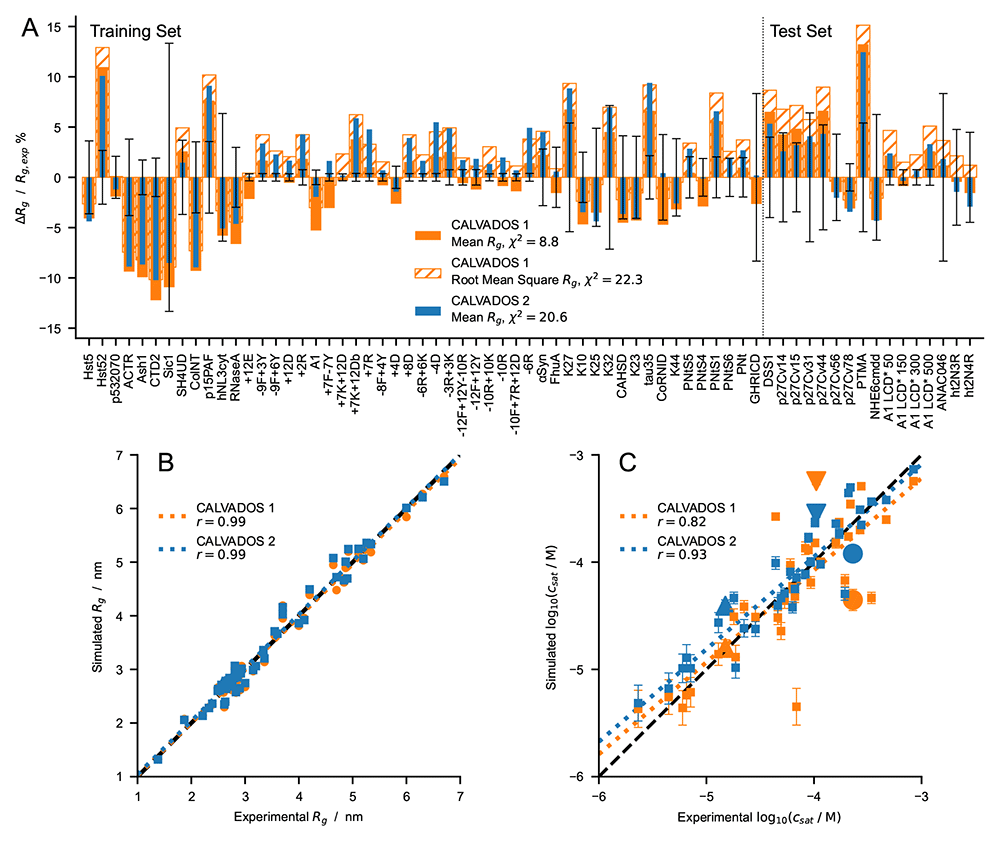
Figure 7.

(A) Relative difference between experimental and predicted radii of gyration for CALVADOS 1 (orange) and CALVADOS 2 (blue). Full and hatched bars show ( $R_{g}^{c a l c}$ − $R_{g}^{e x p}$ ) / $R_{g}^{e x p}$ where $R_{g}^{c a l c}$ is calculated as the mean $〈 R_{g}^{2} 〉$ or the root mean square $\sqrt{〈 R_{g}^{2} 〉}$ , respectively. The vertical dashed line splits the plot into the 51 and 16 sequences or solution conditions of the training set (Table 1) and test set (Table 2), respectively. Error bars represent the experimental error relative to $R_{g}^{e x p}$ . χ² values in the legend are averages over 67 different sequences or solution conditions (Table 1 and Table 2). (B and C) Comparison between experimental and predicted (B) R_g (Table 1 and Table 2) and (C) c_sat values for CALVADOS 1 (orange) and CALVADOS 2 (blue). Pearson’s r coefficients are reported in the legend. Small squares in C show the same data as in Figure 6C–F whereas the large upward triangle, downward triangle, and circle show values for A2 LCD, FUS LCD, and Ddx4 LCD, respectively, at the conditions reported in Table 4.

The correlation between experimental and predicted R_g values for the 67 proteins of Table 1 and Table 2 is excellent for both CALVADOS 1 and 2 (Figure 7B). On the other hand, CALVADOS 2 is more accurate than CALVADOS 1 at predicting PS propensities, as evidenced by Pearson’s correlation coefficients of 0.93 and 0.82, respectively, for the experimental and predicted c_sat values of the 26 sequences of Table 4 (Figure 7C).

Capturing the interplay between short-range nonionic and long-range ionic interactions is essential for accurately modeling the PS of IDPs^58,78–80. Our results show that the decrease in the range of the nonionic potential reported in this work does not significantly perturb the balance between ionic and nonionic forces. In fact, CALVADOS 1 and 2 accurately predict the PS propensities of A1 LCD* at various salt concentrations, as well as the c_sat of variants of A1 LCD and LAF-1 RGG domain with different charge patterning (Figure 3E–G and Figure 6D–F). Moreover, CALVADOS 1 and 2 recapitulate the effect of salt concentration and charge patterning on the chain compaction of A1 LCD*⁶⁸ and p27-C constructs⁶⁷, respectively (Figure 8A and 8B).

As additional test systems, we considered constructs of the 1–80 N-terminal fragment of yeast Lge1, which have been recently investigated using turbidity measurements⁷¹. CALVADOS 2 correctly predicts that the WT Lge1₁₋₈₀ construct undergoes PS at the experimental conditions, albeit with a hundred times larger c_sat (50 ± 6 µM at c_s = 100 mM) compared to experiments (< 1 µM). In agreement with experiments, CALVADOS 2 predicts that mutating all the 11 R residues to K increases c_sat by over one order of magnitude whereas mutating the 14 Y residues of the 1–80 fragment to A abrogates PS (Figure 8C).

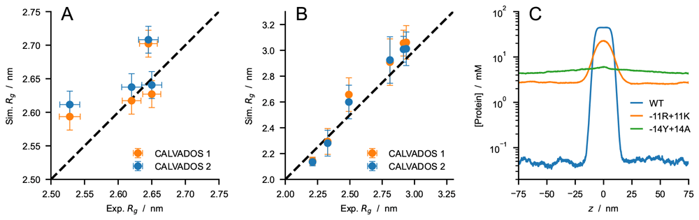
Figure 8.

Comparison between experimental R_g values and predictions of CALVADOS 1 (orange) and CALVADOS 2 (blue) for (A) A1 LCD∗ at different salt concentrations (50 mM < c_s < 500 mM) and (B) p27-C constructs of different charge patterning (0.1 < κ < 0.8). Experimental conditions and references are reported in Table 2. (C) Predictions of CALVADOS 2 direct-coexistence simulations of the PS of constructs of the 1–80 N-terminal fragment of yeast Lge1 simulated at c_s = 100 mM. Protein concentration profiles are shown as a function of the long side of the simulation cell for WT (blue), -11R+11K variant (orange), and -14Y+14A variant (green).

4 Conclusions

In the context of a previously developed Cα-based IDP model (CALVADOS), we show that neglecting the long range of attractive Lennard-Jones interactions has a small impact on the compaction of a single chain while strongly disfavouring PS. The effect can be explained by the smaller number of neglected pair interactions for a residues in an isolated chain compared to the dense environment of a condensate. Moreover, we find that the effect of reducing the range of interaction by a factor of two is relatively insensitive to sequence length and composition. Therefore, decreasing the cutoff of the Lennard-Jones potential of the Cα-based model engenders a similar generic effect on chain compaction and PS as a corresponding increase in temperature. We take advantage of this finding to solve the temperature mismatch of the CALVADOS model. Namely, we decrease the cutoff of the nonionic interactions from 4 to 2 nm and obtain accurate c_sat predictions at the experimental conditions, whereas simulations at temperatures higher by 30 °C were required in the original implementation. Finally, we used the shorter cutoff to reoptimize the “stickiness” parameters of the model against experimental data reporting on single-chain compaction. The small expansion of the chain conformations is overcompensated by an overall increase in “stickiness” so that the resulting model tends to underestimate the experimental c_sat values. By systematically increasing the cutoff used in the development of the “stickiness” scale, we find that performing the optimization using r_c = 2.4 nm results in a model (CALVADOS 2) which yields accurate predictions from simulations run using r_c = 2 nm at the experimental conditions. We present CALVADOS 2 as an improvement of our previous model by testing on sets of experimental R_g and c_sat data comprising 16 and 36 systems, respectively, which were not used in the parameterization of the model.

Data availability

Underlying data

Code and data to reproduce the results presented in this work are available at github.com/KULL-Centre/papers/tree/main/2022/CG-cutoffs-Tesei-et-al and archived on Zenodo at doi.org/10.5281/zenodo.6901205⁸¹ under the terms of the Creative Commons Attribution 4.0 International license.

Extended data

Supplementary figures S1–S7 are deposited on Zenodo at doi.org/10.5281/zenodo.6901205⁸¹ under the terms of the Creative Commons Attribution 4.0 International license.

Software availability

Scripts and parameters to perform single-chain and direct-coexistence simulations using CALVADOS 1 and 2 are available at github.com/KULL-Centre/CALVADOS and archived on Zenodo at doi.org/10.5281/zenodo.6914054⁸² under the terms of the GNU Affero General Public License v3.0.

Ethics and consent

Ethical approval and consent were not required.

Acknowledgments

We thank Anna Ida Trolle for her help in setting up the protocol for single-chain simulations. We thank Rosana Collepardo, Jerelle A. Joseph, and Aleks Reinhardt for useful discussions that led us to explore the effects of cutoffs. We acknowledge access to computational resources from the ROBUST Resource for Biomolecular Simulations (supported by the Novo Nordisk Foundation; NNF18OC0032608) and Biocomputing Core Facility at the Department of Biology, University of Copenhagen. An earlier version of this article can be found on bioRxiv at doi.org/10.1101/2022.07.09.499434.

Faculty Opinions recommended

References

1. Wang J, Choi JM, Holehouse AS, et al.: A molecular grammar governing the driving forces for phase separation of prion-like RNA binding proteins. Cell. 2018; 174(3): 688–699.e16. PubMed Abstract | Publisher Full Text | Free Full Text
2. Monahan Z, Ryan VH, Janke AM, et al.: Phosphorylation of the FUS low-complexity domain disrupts phase separation, aggregation, and toxicity. EMBO J. 2017; 36(20): 2951–2967. PubMed Abstract | Publisher Full Text | Free Full Text
3. Ryan VH, Dignon GL, Zerze GH, et al.: Mechanistic view of hnRNPA2 low- complexity domain structure, interactions, and phase separation altered by mutation and arginine methylation. Mol Cell. 2018; 69(3): 465–479.e7. PubMed Abstract | Publisher Full Text | Free Full Text
4. Martin EW, Holehouse AS, Peran I, et al.: Valence and patterning of aromatic residues determine the phase behavior of prion-like domains. Science. 2020; 367(6478): 694–699. PubMed Abstract | Publisher Full Text | Free Full Text
5. Mittag T, Pappu RV: A conceptual framework for understanding phase separation and addressing open questions and challenges. Mol Cell. 2022; 82(12): 2201–2214. PubMed Abstract | Publisher Full Text | Free Full Text
6. Patel A, Lee HO, Jawerth L, et al.: A liquid-to-solid phase transition of the ALS protein FUS accelerated by disease mutation. Cell. 2015; 162(5): 1066–1077. PubMed Abstract | Publisher Full Text
7. Murakami T, Qamar S, Lin JQ, et al.: ALS/FTD mutation-induced phase transition of FUS liquid droplets and reversible hydrogels into irreversible hydrogels impairs RNP granule function. Neuron. 2015; 88(4): 678–690. PubMed Abstract | Publisher Full Text | Free Full Text
8. Kanaan NM, Hamel C, Grabinski T, et al.: Liquid-liquid phase separation in- duces pathogenic tau conformations in vitro. Nat Commun. 2020; 11(1): 2809. PubMed Abstract | Publisher Full Text | Free Full Text
9. Wegmann S, Eftekharzadeh B, Tepper K, et al.: Tau protein liquid-liquid phase separation can initiate tau aggre- gation. EMBO J. 2018; 37(7): e98049. PubMed Abstract | Publisher Full Text | Free Full Text
10. Peskett TR, Rau F, O'Driscoll J, et al.: A liquid to solid phase transition underlying pathological huntingtin exon1 aggregation. Mol Cell. 2018; 70(4): 588–601.e6. PubMed Abstract | Publisher Full Text | Free Full Text
11. Ray S, Singh N, Kumar R, et al.: α-synuclein aggregation nucleates through liquid-liquid phase separation. Nat Chem. 2020; 12(8): 705–716. PubMed Abstract | Publisher Full Text
12. Hardenberg MC, Sinnige T, Casford S, et al.: Observation of an α-synuclein liquid droplet state and its maturation into lewy body-like assemblies. J Mol Cell Biol. 2021; 13(4): 282–294. PubMed Abstract | Publisher Full Text | Free Full Text
13. Wen J, Hong L, Krainer G, et al.: Conformational expansion of tau in condensates promotes irreversible aggregation. J Am Chem Soc. 2021; 143(33): 13056–13064. PubMed Abstract | Publisher Full Text
14. Dada ST, Hardenberg MC, Mrugalla LK, et al.: Spontaneous nucleation and fast aggregate-dependent proliferation of α-synuclein aggregates within liquid condensates at physiological ph. bioRxiv. 2021. Publisher Full Text
15. Wang B, Zhang L, Dai T, et al.: Liquid-liquid phase separation in human health and diseases. Signal Transduct Target Ther. 2021; 6(1): 290. PubMed Abstract | Publisher Full Text | Free Full Text
16. Lu J, Qian J, Xu Z, et al.: Emerging roles of liquid-liquid phase separation in cancer: From protein aggregation to immune-associated signaling. Front Cell Dev Biol. 2021; 9: 631486. PubMed Abstract | Publisher Full Text | Free Full Text
17. Ahn JH, Davis ES, Daugird TA, et al.: Phase separation drives aberrant chromatin looping and cancer development. Nature. 2021; 595(7868): 591–595. PubMed Abstract | Publisher Full Text | Free Full Text
18. Banani SF, Afeyan LK, Hawken SW, et al.: Genetic variation associated with condensate dysregulation in disease. Dev Cell. 2022; 57(14): 1776–1788.e8. PubMed Abstract | Publisher Full Text
19. Fawzi NL, Parekh SH, Mittal J: Biophysical studies of phase separation integrating experimental and computational methods. Curr Opin Struct Biol. 2021; 70: 78–86. PubMed Abstract | Publisher Full Text | Free Full Text
20. Dignon GL, Zheng W, Kim YC, et al.: Sequence determinants of protein phase behavior from a coarse-grained model. PLoS Comput Biol. 2018; 14(1): e1005941. PubMed Abstract | Publisher Full Text | Free Full Text
21. Choi JM, Dar F, Pappu RV: LASSI: A lattice model for simulating phase transitions of multivalent proteins. PLoS Comput Biol. 2019; 15(10): e1007028. PubMed Abstract | Publisher Full Text | Free Full Text
22. Holehouse AS, Pappu RV: Pimms (0.24 pre-beta). December 2019. Publisher Full Text
23. Holehouse AS, Ginell GM, Griffith D, et al.: Clustering of aromatic residues in prion-like domains can tune the formation, state, and organization of biomolecular condensates. Biochemistry. 2021; 60(47): 3566–3581. PubMed Abstract | Publisher Full Text | Free Full Text
24. Kar M, Dar F, Welsh TJ, et al.: Phase-separating RNA-binding proteins form heterogeneous distributions of clusters in subsaturated solutions. Proc Natl Acad Sci U S A. 2022; 119(28): e2202222119. PubMed Abstract | Publisher Full Text | Free Full Text
25. Bremer A, Farag M, Borcherds WM, et al.: Deciphering how naturally occurring sequence features impact the phase behaviors of disordered prion-like domains. bioRxiv. 2021. Publisher Full Text
26. Farag M, Cohen SR, Borcherds WM, et al.: Condensates of disordered proteins have small-world network structures and interfaces defined by expanded conformations. bioRxiv. 2022. Publisher Full Text
27. Das S, Lin YH, Vernon RM, et al.: Comparative roles of charge, π. and hydrophobic interactions in sequence-dependent phase separation of intrinsically disordered proteins. Proc Natl Acad Sci U S A. 117(46): 28795–28805. PubMed Abstract | Publisher Full Text | Free Full Text
28. Latham AP, Zhang B: Consistent force field captures homologue-resolved hp1 phase separation. J Chem Theory Comput. 2021; 17(5): 3134–3144. PubMed Abstract | Publisher Full Text | Free Full Text
29. Dannenhoffer-Lafage T, Best RB: A data-driven hydrophobicity scale for predicting liquid-liquid phase separation of proteins. J Phys Chem B. 2021; 125(16): 4046–4056. PubMed Abstract | Publisher Full Text
30. Regy RM, Thompson J, Kim YC, et al.: Improved coarse-grained model for studying sequence dependent phase separation of disordered proteins. Protein Sci. 2021; 30(7): 1371–1379. PubMed Abstract | Publisher Full Text | Free Full Text
31. Joseph JA, Reinhardt A, Aguirre A, et al.: Physics-driven coarse-grained model for biomolecular phase separation with near-quantitative accuracy. Nat Comput Sci. 2021; 1(11): 732–743. PubMed Abstract | Publisher Full Text | Free Full Text
32. Tesei G, Schulze TK, Crehuet R, et al.: Accurate model of liquid-liquid phase behavior of intrinsically disordered proteins from optimization of single-chain properties. Proc Natl Acad Sci U S A. 2021; 118(44). PubMed Abstract | Publisher Full Text | Free Full Text
33. Norgaard AB, Ferkinghoff-Borg J, Lindorff-Larsen K: Experimental parameterization of an energy function for the simulation of unfolded proteins. Biophys J. 2008; 94(1): 182–192. PubMed Abstract | Publisher Full Text | Free Full Text
34. Tejedor AR, Garaizar A, Ram´ırez J, et al.: ‘RNA modulation of transport properties and stability in phase-separated condensates. Biophys J. 2021; 120(23): 5169–5186. PubMed Abstract | Publisher Full Text | Free Full Text
35. Das S, Amin AN, Lin YH, et al.: Coarse-grained residue-based models of disordered protein condensates: utility and limitations of simple charge pattern parameters. Phys Chem Chem Phys. 2018; 20(45): 28558–28574. PubMed Abstract | Publisher Full Text
36. Anderson JA, Glaser J, Glotzer SC: HOOMD-blue: A python package for high-performance molecular dynamics and hard particle monte carlo simulations. Comput Mater Sci. 2020; 173: 109363. Publisher Full Text
37. Eastman P, Swails J, Chodera JD, et al.: OpenMM 7: Rapid development of high performance algorithms for molecular dynamics. PLoS Comput Biol. 2017; 13(7): e1005659. PubMed Abstract | Publisher Full Text | Free Full Text
38. Flyvbjerg H, Petersen HG: Error estimates on averages of correlated data. J Chem Phys. 1989; 91(1): 461–466. Publisher Full Text
39. Ashbaugh HS, Hatch HW: Natively unfolded protein stability as a coil-to-globule transition in charge/hydropathy space. J Am Chem Soc. 2008; 130(29): 9536–9542. PubMed Abstract | Publisher Full Text
40. Kim YC, Hummer G: Coarse-grained models for simulations of multiprotein complexes: Application to ubiquitin binding. J Mol Biol. 2008; 375(5): 1416–1433. PubMed Abstract | Publisher Full Text | Free Full Text
41. Akerlof GC, Oshry HI: The dielectric constant of water at high temperatures and in equilibrium with its vapor. J Am Chem Soc. 1950; 72(7): 2844–2847. Publisher Full Text
42. Nagai H, Kuwabara K, Carta G: Temperature dependence of the dissociation constants of several amino acids. J Chem Eng Data. 2008; 53(3): 619–627. Publisher Full Text
43. Simm S, Einloft J, Mirus O, et al.: 50 years of amino acid hydrophobicity scales: revisiting the capacity for peptide classification. Biol Res. 2016; 49(1): 31. PubMed Abstract | Publisher Full Text | Free Full Text
44. Pedregosa F, Varoquaux G, Gramfort A, et al.: Scikit-learn: Machine learning in Python. J Mach Learn Res. 2011; 12: 2825–2830. Reference Source
45. Jephthah S, Staby L, Kragelund BB, et al.: Temperature dependence of intrinsically disordered proteins in simulations: What are we missing? J Chem Theory Comput. 2019; 15(4): 2672–2683. PubMed Abstract | Publisher Full Text
46. Fagerberg E, Månsson LK, Lenton S, et al.: The effects of chain length on the structural properties of intrinsically disordered proteins in concentrated solutions. J Phys Chem B. 2020; 124(52): 11843–11853. PubMed Abstract | Publisher Full Text | Free Full Text
47. Zhao J, Blayney A, Liu X, et al.: EGCG binds intrinsically disordered N-terminal domain of p53 and disrupts p53-MDM2 interaction. Nat Commun. 2021; 12(1): 986. PubMed Abstract | Publisher Full Text | Free Full Text
48. Kjaergaard M, Nørholm AB, Hendus–Altenburger R, et al.: Temperature-dependent structural changes in intrinsically disordered proteins: Formation of alpha-helices or loss of polyproline II? Protein Sci. 2010; 19(8): 1555–1564. PubMed Abstract | Publisher Full Text | Free Full Text
49. Martin EW, Holehouse AS, Grace CR, et al.: Sequence determinants of the conformational properties of an intrinsically disordered protein prior to and upon multisite phosphorylation. J Am Chem Soc. 2016; 138(47): 15323–15335. PubMed Abstract | Publisher Full Text | Free Full Text
50. Jin F, Gräter F: How multisite phosphorylation impacts the conformations of intrinsically disordered proteins. PLoS Comput Biol. 2021; 17(5): e1008939. PubMed Abstract | Publisher Full Text | Free Full Text
51. Gibbs EB, Lu F, Portz B, et al.: Phosphorylation induces sequence-specific conformational switches in the RNA polymerase II c-terminal domain. Nat Commun. 2017; 8(1): 15233. PubMed Abstract | Publisher Full Text | Free Full Text
52. Gomes GW, Krzeminski M, Namini A, et al.: Conformational ensembles of an intrinsically disordered protein consistent with NMR, SAXS, and single-molecule FRET. J Am Chem Soc. 2020; 142(37): 15697–15710. PubMed Abstract | Publisher Full Text
53. Shrestha UR, Juneja P, Zhang Q, et al.: Generation of the configurational ensemble of an intrinsically disordered protein from unbiased molecular dynamics simulation. Proc Natl Acad Sci U S A. 2019; 116(41): 20446–20452. PubMed Abstract | Publisher Full Text | Free Full Text
54. Johnson CL, Solovyova AS, Hecht O, et al.: The two-state prehensile tail of the antibacterial toxin colicin N. Biophys J. 2017; 113(8): 1673–1684. PubMed Abstract | Publisher Full Text | Free Full Text
55. De Biasio A, Ibáñez de Opakua A, Cordeiro TN, et al.: p15^PAF is an intrinsically disordered protein with nonrandom structural preferences at sites of interaction with other proteins. Biophys J. 2014; 106(4): 865–874. PubMed Abstract | Publisher Full Text | Free Full Text
56. Paz A, Zeev-Ben-Mordehai T, Lundqvist M, et al.: Biophysical characterization of the unstructured cytoplasmic domain of the human neuronal adhesion protein neuroligin 3. Biophys J. 2008; 95(4): 1928–1944. PubMed Abstract | Publisher Full Text | Free Full Text
57. Riback JA, Bowman MA, Zmyslowski AM, et al.: Innovative scattering analysis shows that hydrophobic disordered proteins are expanded in water. Science. 2017; 358(6360): 238–241. PubMed Abstract | Publisher Full Text | Free Full Text
58. Bremer A, Farag M, Borcherds WM, et al.: Deciphering how naturally occurring sequence features impact the phase behaviours of disordered prion-like domains. Nat Chem. 2022; 14(2): 196–207. PubMed Abstract | Publisher Full Text | Free Full Text
59. Ahmed MC, Skaanning LK, Jussupow A, et al.: Refinement of α-synuclein ensembles against SAXS data: Comparison of force fields and methods. Front Mol Biosci. 2021; 8: 654333. PubMed Abstract | Publisher Full Text | Free Full Text
60. Mylonas E, Hascher A, Bernadó P, et al.: Domain conformation of tau protein studied by solution small-angle x-ray scattering. Biochemistry. 2008; 47(39): 10345–10353. PubMed Abstract | Publisher Full Text
61. Hesgrove C, Nguyen KH, Biswas S, et al.: Tardigrade CAHS proteins act as molecular swiss army knives to mediate desiccation tolerance through multiple mechanisms. bioRxiv. 2021. Publisher Full Text
62. Lyu C, Da Vela S, Al-Hilaly Y, et al.: The disease associated tau35 fragment has an increased propensity to aggregate compared to full-length tau. Front Mol Biosci. 2021; 8: 779240. PubMed Abstract | Publisher Full Text | Free Full Text
63. Cordeiro TN, Sibille N, Germain P, et al.: Interplay of protein disorder in retinoic acid receptor heterodimer and its corepressor regulates gene expression. Structure. 2019; 27(8): 1270–1285.e6. PubMed Abstract | Publisher Full Text
64. Bowman MA, Riback JA, Rodriguez A, et al.: Properties of protein unfolded states suggest broad selection for expanded conformational ensembles. Proc Natl Acad Sci U S A. 2020; 117(38): 23356–23364. PubMed Abstract | Publisher Full Text | Free Full Text
65. Seiffert P, Bugge K, Nygaard M, et al.: Orchestration of signaling by structural disorder in class 1 cytokine receptors. Cell Commun Signal. 2020; 18(1): 132. PubMed Abstract | Publisher Full Text | Free Full Text
66. Pesce F, Newcombe EA, Seiffert P, et al.: Assessment of models for calculating the hydrodynamic radius of intrinsically disordered proteins. bioRxiv. 2022. Publisher Full Text
67. Das RK, Huang Y, Phillips AH, et al.: Cryptic sequence features within the disordered protein p27^Kip1 regulate cell cycle signaling. Proc Natl Acad Sci U S A. 2016; 113(20): 5616–5621. PubMed Abstract | Publisher Full Text | Free Full Text
68. Martin EW, Thomasen FE, Milkovic NM, et al.: Interplay of folded domains and the disordered low-complexity domain in mediating hnRNPA1 phase separation. Nucleic Acids Res. 2021; 49(5): 2931–2945. PubMed Abstract | Publisher Full Text | Free Full Text
69. Kurzbach D, Vanas A, Flamm AG, et al.: Detection of correlated conformational fluctuations in intrinsically disordered proteins through paramagnetic relaxation interference. Phys Chem Chem Phys. 2016; 18(8): 5753–5758. PubMed Abstract | Publisher Full Text
70. Dedmon MM, Lindorff-Larsen K, Christodoulou J, et al.: Mapping long-range interactions in alpha-synuclein using spin-label NMR and ensemble molecular dynamics simulations. J Am Chem Soc. 2005; 127(2): 476–477. PubMed Abstract | Publisher Full Text
71. Polyansky AA, Gallego LD, Efremov RG, et al.: Protein compactness and interaction valency define the architecture of a biomolecular condensate across scales. bioRxiv. 2022. Publisher Full Text
72. Martin EW, Harmon TS, Hopkins JB, et al.: A multi-step nucleation process determines the kinetics of prion-like domain phase separation. Nat Commun. 2021; 12(1): 4513. PubMed Abstract | Publisher Full Text | Free Full Text
73. Schuster BS, Dignon GL, Tang WS, et al.: Identifying sequence perturbations to an intrinsically disordered protein that determine its phase-separation behavior. Proc Natl Acad Sci U S A. 2020; 117(21): 11421–11431. PubMed Abstract | Publisher Full Text | Free Full Text
74. Ryan VH, Perdikari TM, Naik MT, et al.: Tyrosine phosphorylation regulates hnRNPA2 granule protein partitioning and reduces neurodegeneration. EMBO J. 2021; 40(3): e105001. PubMed Abstract | Publisher Full Text | Free Full Text
75. Murthy AC, Dignon GL, Kan Y, et al.: Molecular interactions underlying liquid-liquid phase separation of the FUS low-complexity domain. Nat Struct Mol Biol. 2019; 26(7): 637–648. PubMed Abstract | Publisher Full Text | Free Full Text
76. Brady JP, Farber PJ, Sekhar A, et al.: Structural and hydrodynamic properties of an intrinsically disordered region of a germ cell-specific protein on phase separation. Proc Natl Acad Sci U S A. 2017; 114(39): E8194–E8203. PubMed Abstract | Publisher Full Text | Free Full Text
77. Wang X, Ramírez-Hinestrosa S, Dobnikar J, et al.: The lennard-jones potential: when (not) to use it. Phys Chem Chem Phys. 2020; 22(19): 10624–10633. PubMed Abstract | Publisher Full Text
78. Mercadante D, Wagner JA, Aramburu IV, et al.: Sampling long-versus short-range interactions defines the ability of force fields to reproduce the dynamics of intrinsically disordered proteins. J Chem Theory Comput. 2017; 13(9): 3964–3974. PubMed Abstract | Publisher Full Text
79. Alshareedah I, Kaur T, Ngo J, et al.: Interplay between short-range attraction and long-range repulsion controls reentrant liquid condensation of ribonucleoprotein–RNA complexes. J Am Chem Soc. 2019; 141(37): 14593–14602. PubMed Abstract | Publisher Full Text | Free Full Text
80. Hazra MK, Levy Y: Biophysics of phase separation of disordered proteins is governed by balance between short- and long-range interactions. J Phys Chem B. 2021; 125(9): 2202–2211. PubMed Abstract | Publisher Full Text | Free Full Text
81. Tesei G, Lindorff-Larsen K: Improved Predictions of Phase Behaviour of IDPs by Tuning the Interaction Range. 2022. http://www.doi.org/10.5281/zenodo.6901205
82. Tesei G, Schulze TK, Crehuet R, et al.: CALVADOS: Coarse-graining Approach to Liquid-liquid phase separation Via an Automated Data-driven Optimisation Scheme. 2022. http://www.doi.org/10.5281/zenodo.6914054

Comments

Publication information

Section

Research Article

Published

August 5, 2022

DOI

https://doi.org/10.12688/openreseurope.14967.1

Versions

January 17, 2023 (Version of Record 2.0)
August 5, 2022 (Version of Record 1.0)

Included in

Funding data

European Commission

Grant ID(s): 101025063

Metrics

Views

1,193

Downloads

343

Citations

See full metrics

Keywords

intrinsically disordered proteins, liquid–liquid phase separation, force field parameterization, biomolecular condensates, protein interactions

Comments

Giulio Tesei

Structural Biology and NMR Laboratory & the Linderstrøm-Lang Centre for Protein Science, Department of Biology, University of Copenhagen, Copenhagen, Denmark

Roles

Corresponding Author, Co-Author, Conceptualization, Formal Analysis, Funding Acquisition, Investigation, Methodology, Project Administration, Visualization, Writing – Original Draft Preparation, Writing – Review & Editing

0000-0003-4339-4460

giulio.tesei@bio.ku.dk

Kresten Lindorff-Larsen

Structural Biology and NMR Laboratory & the Linderstrøm-Lang Centre for Protein Science, Department of Biology, University of Copenhagen, Copenhagen, Denmark

Roles

Co-Author, Conceptualization, Funding Acquisition, Investigation, Methodology, Project Administration, Resources, Supervision, Writing – Review & Editing

0000-0002-4750-6039

lindorff@bio.ku.dk

Downloads over the last 12 months:

Cited by

via Crossref

View citing articles

Improved predictions of phase behaviour of intrinsically disordered proteins by tuning the interaction range

List of Authors

Peer review

Publication information

Included in

Funding data

Metrics

Keywords

Comments

Abstract

Comments

Publication information

Included in

Funding data

Metrics

Keywords

Comments

Authors & roles

Giulio Tesei

Kresten Lindorff-Larsen

Downloads over the last 12 months:

Cited by

via Crossref