Plain language summary
This article analyses performances on a hand-turned mechanical musical instrument, using a similar approach to earlier research (for example, Spiro et al., 2010; Volioti, 2019) concerned with mapping tempo and timing changes in other kinds of instrumental performances. These methods help to measure the patterns of speeding up and slowing down across the piece that characterise a recorded performance, and in this way make it possible to compare some aspects of what different performers do with different music, with different instruments, and in different contexts. The reason for conducting this research was that mechanical instruments are not usually considered to be important for performance, but they were used by many street performers who were often criticised as being unmusical or for producing unwanted sounds. So as well as beginning to explore some of the distinctive ways of playing that might be associated with manually-operated mechanical instruments, these findings also represent an invitation for future research to reconsider the music of street barrel organists in history as a legitimate performance tradition that should be recognised and valued.
Introduction
This article investigates the extent to which a performance on a hand-cranked mechanical instrument might compare (in temporal terms) to more widely-recognised types of instrumental performance. A key question was: to what extent is it possible to play ‘expressively’ with these instruments? This is not a purely philosophical question but also a historically, socially and culturally contingent one, tied to notions of value, skill and authenticity in performance, and implicitly of who is valued in a society. Across fin-de-siècle Europe and North America, organ grinders were criticised for playing ‘unmusically’ (Accinno, 2015; Cohen & Greenwood, 1981; Ord-Hume, 1978). Up to the present day, mechanical (and digital) instruments have been associated with the idea of robotic, unexpressive, ‘deadpan’ or ‘nominal’ performances (Cook, 2013). But Ord-Hume (1978) has argued that it is possible to create a ‘musical’ or expressive rendition using a barrel organ. Shifts in musicology towards recognising that creative labour and agency in music are not restricted to top-down models with rigidly defined roles are reflected in interventions on listening (Clarke, 1989; Maloney, 2017), audiences (Born, 2021) and notation (Schuiling, 2019). Research by Williams (2016) on reconstructing Stockhausen’s Studie II is conceptually aligned with the present study in that it challenges the exclusion of a clearly active agent in musicking (a technician, an organ grinder) from some implicit paradigm of musical creativity. Following the impact of more psychological or anthropological, audience- or listening-focused, studies, listeners are constructed as active, agential participants in musicking; it is also now acknowledged that performers often take on aspects of the ‘traditional’ role of a composer and/or arranger. The present study continues to reconsider boundaries around what the role of a performer/musician does and does not constitute (an issue also addressed by Butler [2014] and De Souza [2017]). These kinds of approaches resist the idea that the barrel organ is not a ‘real’ instrument or that an organ grinder is not a ‘real’ musician.
Digital musicology literature has seen many methodologically innovative studies using applications like Sonic Visualiser in conjunction with machine learning tools to investigate timing patterns in recorded performances of European classical music, often measuring the distances between note onsets to map tempo changes over time. The purpose of the experiments carried out was to see what might emerge when applying the same analytical techniques not to a piano performance of a Chopin mazurka, but to a sample of recordings of different people playing a hand-cranked mechanical musical instrument. This research is speculative in the sense that there is not a particular consensus that hand-cranked instruments can be played ‘expressively’. Mechanical musical instruments, despite being beloved by enthusiast communities, preserved in museums and highly regarded as luxury antique objects in many cases, have not necessarily been regarded as important in the history of music as a performance-based phenomenon. This study starts down avenues of investigation that could bring further nuance to longstanding questions around where ‘performance’ starts and ends.
First it is necessary to acknowledge that ‘playing expressively’ is a subjective, and historically and culturally contingent, concept. However, this article asks not the primary question, ‘what is expressive playing?’, but the secondary one, ‘given that certain temporal characteristics in existing recordings have previously been understood in terms of expressiveness, to what extent are comparable characteristics perceptible in a sample of recordings of a different kind of performance?’. Timing is widely considered a critical element of expressiveness in discourses of European classical music performance, with popular concepts like rubato having received extensive discussion elsewhere (Hudson, 1994). Unlike a fully automated clockwork instrument or a MIDI sequencer, a hand-cranked instrument does not play a perfectly regular sequence of beats. The question of whether certain timing-related phenomena or decisions in performance are ‘expressive’ has been examined from different angles, including influential music psychology studies around listener perception of timing fluctuation (Clarke, 1989) and attempts to create structural models for ‘expressive’ timing that could be mapped onto computer-generated performances to create a ‘musically acceptable’ result (Desain & Honing, 1993; Todd, 1985). Although instruments like barrel organs have been denigrated as producing inferior renditions, this study asks whether fluctuations in human-controlled mechanical performance might be seen not exclusively as errors, but as potentially significant in terms of expression.
Methods
Music box
Performance analysis has seen many studies concerned with quantifying temporal features of recorded renditions of pieces of music (often of canonic classical works, since this typically means a large available sample of the same piece recorded by different players for comparison purposes, and often of Chopin’s piano works, perhaps owing to the strong association with rubato surrounding this material). The instrument used for the present experiment was a modern 30-note programmable music box – a metal action with a few plastic parts in a wooden case – which reads punched card rolls. The box’s scale includes every chromatic note at least once but is based around C and G (for example, it contains only one G# but 4 octave Gs). This instrument is not 'historical' and can not cast light on historical performance; this preliminary investigation is intended to be built upon by future studies that will collect data from an Ariston Organette and a number of instruments held in museum collections, including barrel organs and barrel pianos that were used by nineteenth- and twentieth-century street performers.
Repertoire and collection of recordings
I arranged two extracts – from Scott Joplin’s ‘Bethena’ Concert Waltz (24 bars, bars 53 to 76, see Figure 1); and the first 24 bars of Frederik Chopin’s Valse in A minor opus 34 no. 2 (see Figure 2), both of which are in triple time, have a sounding crotchet on almost every beat of every bar, and have a similar A-A-B structure. I asked six participants to play each extract twice for a recording, and then analysed these recordings using means – Sonic Visualiser and Self Organizing Maps – that have previously been used to analyse other kinds of instrumental performances (piano, for example). The reasoning behind the choice of repertoire was to select pieces that were idiomatically comparable to items from traditional barrel organ repertoire and that have useful musical features for analytical purposes. Waltzes were a popular form associated with mechanical instruments. Additionally, Chopin’s piano music in particular has come to be associated with rubato and frequently features in relevant studies on timing in musical performance (Leech-Wilkinson, 2015; Spiro et al., 2010), so it was considered an appropriate choice in the context of existing literature on measuring and describing rubato. The two extracts, notwithstanding many similarities, also have distinct rhythmic characters; ‘Bethena’ is consistently and distinctively syncopated, while ‘Valse’ is more regular. Additional reasons for these choices were to select pieces that could be approximated fairly closely on the music box, with its limited set of pitches and inability to play fast successive pitches or very dense chords; and pieces that had a note onset on every beat of the bar almost constantly in order to facilitate onset measurement. Both pieces are in a triple metre for consistency and are often played at a moderate tempo that is within the idiomatic window of the music box; future experiments could include different kinds of metre, or more contrasting styles, for broader comparison.
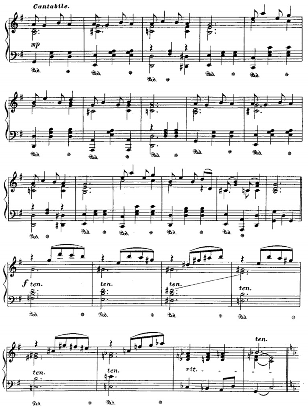
It’s not necessarily the case that either of these pieces were ever played on a street barrel piano, domestic music box or any other type of historical mechanical instrument; the choice of repertoire is more about finding an appropriate sort of musical material that might lend itself to particular conventional interpretations that could potentially ultimately be viewed in relation to some of the idiomatic features of a hand-cranked mechanical instrument. The experiment is not intended to recreate historical conditions but to begin to explore the basic concept of tempo fluctuations in hand-cranked mechanical instruments using repertoire which is stylistically relevant and technically feasible.
Participants
The eligibility of participants was determined by meeting the following criteria: resident in Utrecht; over the age of 18; English-speaking; available and willing to participate in the experiment. Because this research was carried out in the context of coronavirus lockdowns, the pool of participants was drawn from a combination of neighbours, colleagues, and acquaintances for practical and safety reasons, to avoid encouraging anyone to travel and to limit in-person meetings during the pandemic. None of the participants were informed about the questions that would later be asked of the data in order to avoid influencing the performances.
Among the group of six participants in this experiment there was an even split of participants with intensive training in European classical music and those with comparatively little or no experience of this kind. Participants were men and women aged between 25 and 35, who were resident in Utrecht at the time of the experiment. Half the participants are originally from the Netherlands and half are originally from elsewhere in Europe or from India. Only one participant had played a similar music box in advance of the experiment, and two were familiar with and had played at least one of the pieces before. Three of the participants had graduate-level musical performance training (European classical music), one participant had some experience playing the piano but described this as not extensive, and two identified as having no instrumental performance experience. Half the participants were invited to briefly prepare the pieces first during the recording session, and half were played a MIDI loop of the opening at 100 bpm. Table 1 shows details about the participants.
Table 1. Table showing participants’ experience in music and with the pieces.
| Participant | Prepared pieces
before recording | Music/performance
experience (self-described) | Had played a
similar music
box before | Had played
‘Bethena’ before | Had played
‘Valse’ before |
| 1 | (tempo given) | Postgraduate level | | | |
| 2 | (tempo given) | None | | | |
| 3 | (tempo given) | None | | | |
| 4 | | Postgraduate level | | | |
| 5 | | Postgraduate level | | | |
| 6 | | Some | | | |
Ethics statement
All participants took part willingly with the knowledge that their performances were being recorded as part of an experiment for research into mechanical music performance, and that all data would be fully anonymised. Formal ethical approval and consent was not required because no personal or sensitive data was collected.
Data analysis
I used Sonic Visualiser to locate the onsets of each beat of the bar in all of the participant recordings, using Dan Stowell’s Onset Detector transform and manual editing. I created tempo curve graphs for these 24 recordings, plus six recordings by pianists for comparison (‘Valse’: Alice Sara Ott, Dang Thai Son, Artur Rubinstein; ‘Bethena’: Janice Scroggins, William Appling, Joshua Rifkin), and exported the beat tempo layer data to get datasets comprising the BPM tempo of each sounding beat of the bar. I intended to investigate: how much variation across different participants there might be; how much variation across different parts of the extract there might be in a single performance; and how different these recordings might be from highly-prepared professional piano performances of the same music. All of the music box recordings discussed here, and two appendices showing SOM results for all the recordings of ‘Bethena’ and ‘Valse’ respectively can be found in the underlying data set ‘Expressive timing and mechanical instruments’ (McGinn, 2022).
‘Control samples’ using metronome
Although this study draws on methodologically similar analyses of analog instrumental performances, there is not an existing body of literature using comparable techniques to analyse hand-cranked mechanical performances. As such, there are gaps that need to be addressed, partly in the context of the current experiment, but also pointing to further work that would be needed to produce more robust, conclusive results.
In order to create some recordings for comparison purposes that would ideally represent the most-regular-possible performance on the given instrument, I recorded each extract twice using a metronome set to 100 bpm. As mechanical music performers would report, this does not result in a perfectly regular performance, because trying to play a mechanical instrument ‘metrically’ (i.e., with a mental structure of three beats in a bar and with whatever somatic responses stem from that approach) creates non-metrical irregularities – or at least, is not considered to be an effective strategy for playing regularly. In a video by musician and instrument builder Martin Molin (Wintergatan), Joost Oehler, a guide at Museum Speelklok, describes this phenomenon in relation to a much larger hand-cranked organ as follows:
JO: “You always have to grind the wheel at the same tempo, no matter what organ book you play, and the tempo is in the organ book.”
MM: “So, they put the holes closer together to have a faster song. And then you get into your muscular memory exactly so the whole evening you have the same tempo.”
JO: “Yeah, you’re always swinging it at the same tempo, and [the] best thing is to not think about it! And not trying to anticipate like, oh, I’m gonna go slower or I’m gonna go faster. Just listen to it and… wonder if it’s okay. And if it’s not okay, you go a bit faster or a bit slower, but make it a long term decision.”
MM: “Because on my small music box with a crank, I have the same – and I usually, like, have a mantra in my brain and [try] not [to be] listening to [the] music, like… “bread and water, bread and water, bread and water” – but that sounded too rhythmical. I’m thinking of something completely different. “Thinking about the tree, thinking about the tree, thinking about the tree, thinking about the tree”, something like that.”
JO: “You need to do exactly that, when you do this. It’s the same with the music boxes.” (Molin, 2017).
So, it is accepted by musicians and museum professionals with experience of mechanical instruments that a regular, ideally non-metrical pace of handle-turning is required for optimal performance – which does not necessarily contradict Ord-Hume’s claim that an aesthetically pleasing or sensitive performance can be achieved by the ‘sympathetic turning of the handle.’ But the historical tradition of hand-cranked street performance was practised by thousands of people who, although many of them had come from similar regions of or similar backgrounds in Italy, nevertheless were all individual players with creative agency in their own right. As Roberts (2018) has argued in relation to the magic lantern as a popular domestic commodity, a media technology left in the hands of enough people for enough time will likely be stretched to its physical limits and used for almost any imaginable creative end. Although there may be a certain degree of consensus about the ‘right’ way to play a mechanical instrument there is next to no evidence about the musical performance practice of street organ grinders, besides anecdotal reports that they were playing ‘wrong’ or badly. If, in addition to the prejudices of onlookers, part of the reason for this denigration stemmed from the fact that many buskers were not playing in what was considered to be the ‘right’ (regular) way, then it would be interesting to at least begin to approach a preliminary technical recreation of what kinds of things they could possibly have been doing.
Discussions above suggest that the more ‘musically’ or ‘expressively’ you try to play a hand-cranked instrument, the more irregular the output would become. It may be relevant in terms of historical reception discourse that it was and a remains a particular middle-class musical value to demonstrate poised control and mechanical restraint (Bull, 2019) – and that, rather than mechanical performances being robotic, ‘unmusical’ or unexpressive, they were actually too idiomatic or individual for the likings of a demographic whose musical tastes were coalescing, in line with the emergence of sound recording, around a preoccupation with uniformity and repeatability. This research is exploratory and does not represent a historical reconstruction. But it starts to move towards a consideration of hand-cranked mechanical instruments as performance media, not only as proto-recording/playback technologies.
Tempo graph results and phrase-arching
The tempo graphs yielded some basic insights. Unsurprisingly, participants who had been invited to practice the pieces once before recording seemed more likely to produce a recording that indicated some kind of intentional performance strategy. The tempo graphs show, moreover, that participants created performances that could be seen as idiomatic.
Abbreviations key:
JS – Janice Scroggins
WA – William Appling
JR – Joshua Rifkin
ASO – Alice Sara Ott
DTS – Dang Thai Son
AR – Artur Rubinstein
P1B1 – Participant 1, ‘Bethena’, recording 1
CSV2 – ‘Control sample’, ‘Valse’, recording 2
Participant 1 was intensively trained in European classical performance but was not invited to prepare the extracts, and was given a rough tempo to match from a short MIDI clip loop. They had also played a similar music box before. Their performance was very regular, with less fluctuations than some by participants with less musical performance experience, but also displayed less fluctuations than some intensively-classically-trained participants who were invited to prepare the piece. There was not much slowing down at phrase endings (or phrase-arching) which we might think of as a kind of typical expressive timing feature (cf. Cook, 2014). Participant 2, who had little or no instrumental performance experience and was not invited to prepare the piece, showed more fluctuation or ‘irregularity’ than Participant 1, but there didn’t seem to be at first glance any relationship between the fluctuations and any structural points in the music. Participant 4, who was intensively-classically-trained, was invited to prepare the extracts, and said they had played the Chopin Valse before on the piano, showed not only quite a bit of fluctuation but also a sectional approach to the piece in both recordings.
Figure 3 shows tempo graphs for the second recording of the Chopin Valse for Participants 1, 2 and 4. As the graph indicates, Participant 1 produced a flatter, more ‘controlled’ contour, and didn’t consistently introduce phrase-arching. Participant 2 was less familiar with instrumental performance and mechanical instruments and there is greater fluctuation here, but also no clear sense of something structurally-motivated (unsurprisingly, since they were not familiar with the piece). And Participant 4, who had previously played this piece on the piano and was invited to prepare it in the recording session, includes quite a bit of fluctuation, some marked phrase arching, and a clear difference in tempo between the three phrases. Figure 4 shows more tempo graphs for the Chopin Valse, with music box performances (the first recording in each case) on the top row and piano performances on the second row. Participant 6’s graph seems to fluctuate more than it does because the performance was comparatively very slow and accordingly the scale on the y axis is different from the other examples. There is a visible similarity between Participant 4’s structurally segmented music box interpretation and some of the piano interpretations (notably Alice Sara Ott’s).
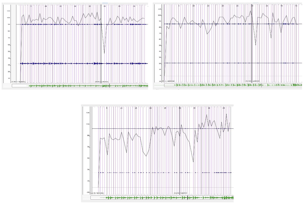
Figure 3. Tempo graphs for recordings of ‘Valse’.
Clockwise from the top right, the images are from participants 1, 2 and 4.
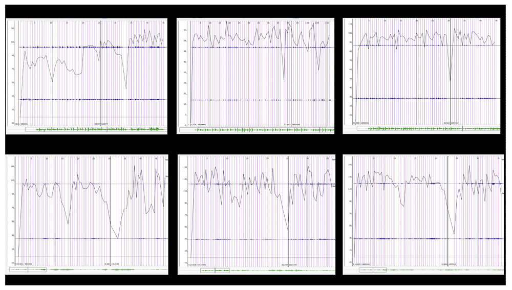
Figure 4. ‘Valse’ tempo graphs for three music box players (P4V1, P6V1, P1V1) and three pianists (Alice Sara Ott, Dang Thai Son and Artur Rubinstein).
The top row from left to right is P4, P6, P1, and the second row from left to right is Alice Sara Ott, Dang Thai Son, Artur Rubinsten.
The following Tables (2 and 3) indicate, in both ‘Bethena’ and ‘Valse’ recordings, whether a given participant slowed down at a particular structural moment in the music. This will be the working understanding of ‘phrase arching’ for our context, and will be used as a preliminary means to investigate whether this recognised form of expressive timing does occur at ‘musically’ coherent points in some music box performances as well as in piano ones. In the case of ‘Bethena’, shown below, the tendency towards phrase-arching at the identified points was insignificant in P3 and P6. Conversely, the tendency towards phrase-arching at the identified points was stronger in P2, P4, P5, and the recordings by pianists, while P1 and the control samples were somewhere inbetween. ‘0’ indicates that the player did not slow down or speed up; ‘1’ indicates that they did (using a difference of 10bpm as a threshold; ‘*’ indicates that this moment of drastic slowing in Participant 4’s first recording of Bethena may simply reflect a moment of greater resistance from the crank mechanism.
Table 2. Table showing end-slowing in performances of ‘Bethena’.
| Bethena | Slowing around
bar 4 | Slowing around
bar 8 | Slowing around bar
12 | Slowing around bar
16 | Slowing around bar
24 |
| P1B1 | 1 | 0 | 0 | 0 | 0 |
| P1B2 | 0 | 1 | 1 | 0 | 1 |
| P2B1 | 1 | 0 | 1 | 1 | 0 |
| P2B2 | 1 | 0 | 1 | 1 | 1 |
| P3B1 | 0 | 0 | 0 | 1 | 0 |
| P3B2 | 0 | 0 | 0 | 0 | 0 |
| P4B1 | 1 | 1 | 1 | 1* | 0 |
| P4B2 | 0 | 1 | 0 | 1 | 1 |
| P5B1 | 1 | 1 | 1 | 1 | 1 |
| P5B2 | 1 | 1 | 1 | 1 | 1 |
| P6B1 | 0 | 0 | 0 | 0 | 1 |
| P6B2 | 1 | 0 | 0 | 0 | 0 |
| CSB1 | 1 | 1 | 1 | 1 | 0 |
| CSB2 | 0 | 1 | 1 | 0 | 1 |
| JS | 1 | 1 | 1 | 1 | 1 |
| WA | 1 | 1 | 1 | 1 | 1 |
| JR | 1 | 1 | 1 | 1 | 1 |
Table 3. Table showing end-slowing in performances of ‘Valse’.
| Valse | Slowing around
bar 8 | Slowing around
bar 16 | Slowing around
bar 24 |
| P1V1 | 1 | 1 | 1 |
| P1V2 | 1 | 1 | 0 |
| P2V1 | 1 | 1 | 1 |
| P2V2 | 1 | 1 | 1 |
| P3V1 | 1 | 0 | 0 |
| P3V2 | 0 | 1 | 0 |
| P4V1 | 1 | 1 | 1 |
| P4V2 | 1 | 1 | 1 |
| P5V1 | 1 | 1 | 1 |
| P5V2 | 1 | 1 | 0 |
| P6V1 | 0 | 1 | 0 |
| P6V2 | 0 | 0 | 0 |
| CSV1 | 0 | 0 | 0 |
| CSV2 | 0 | 0 | 1 |
| ASO | 1 | 1 | 1 |
| DTS | 1 | 1 | 1 |
| AR | 1 | 1 | 1 |
Around bar 16 in Participant 4’s first performance of Bethena, the marked result in the table refers to a significantly slower second beat and a much faster third beat – when the recording is played back, and on the tempo graph, the impression is of the handle getting ‘stuck’ momentarily, and the player reacting by applying more pressure to try and get back to the desired tempo. In Participant 5’s recordings, often a pronounced elongated beat 2 coincides with a passage where slowing down would be conventional. In both cases it may be that the hand-cranked instrument exerts a certain kind of equilibrium that contributes to idiomatic patterns that are not characteristic of, say, piano performance. There is not presently enough evidence to strongly make this claim, but future experiments could measure the results when participants are instructed to try and play particular kinds of temporal shapes.
In ‘Valse’, the phrases do not subdivide as clearly as in ‘Bethena’, and so end-slowing is only measured at three points rather than the five measured in the latter example. Here again participants 4 and 5, who were musicologists and were invited to freely prepare the pieces, show the strongest tendency towards phrase-arching from the music box samples, presumably in part due to being explicitly familiar with this as a convention (and perhaps having some intuition about the purpose of the experiments, although this wasn’t disclosed). However, end-slowing and phrase-arching can be seen as part of a tacit knowledge of musical performance conventions, featuring in many global northern popular, folk, jazz and classical styles. Participants 2 and 3 both described themselves as having no musical performance experience at all, but Participant 2 demonstrates a stronger tendency towards end-slowing than Participant 3. Participant 6, although their recordings do not show this very clearly, mentioned that they were trying to ‘slow down at the end’. In the case of the piano recordings, the trend is consistently towards phrase-arching.
In Participant 4 and 5’s recordings the bpm value results show a more pronounced, gradual and incremental end-slowing. In other music box examples, end-slowing is also frequently measurable but tends to appear in the form of one or two beats with a notably lower tempo rather than a consistent decrease in tempo of 10-30 bpm over the course of the last two bars of a phrase. It could be argued that the former examples are reflective of a deliberate end-slowing while the other instances are anomalous or coincidental. For the purposes of this initial investigation, however, I am observing a threshold of a difference of 10 bpm within or leading into the last bar or a phrase, which could include a case in which the last beat of the penultimate bar is the slowest beat in the phrase. The limitations posed by using this threshold for measuring phrase-arching here are acknowledged. A more nuanced analysis of the variety of patterns that could constitute deliberate or planned end-slowing in different music box performances would be a useful future step. Participant 6, who vocalised their intention to vary the tempo but whose results did not always meet the thresholds used here, nevertheless produced some interesting results. There was some significant slowing in the region of phrase endings, but it usually started earlier, was less gradated, and was followed by a increase in or passage of stable tempo as the phrase ended, looking more like a high degree of fluctuation than something directional. In both recordings of ‘Valse’, Participant 6 decreased and then increased the tempo in the last two bars of the first two phrases, resulting in beat-two-elongation (though the first recording does not quite meet the 10bpm threshold in either case). The fact that this tendency, although it does not quite resemble end-slowing, is repeated in both recordings, suggests that it may reflect some kind of interpretive strategy – further supporting the conclusion that interpretive strategies, idiomatic renditions or ‘expressive’ playing are possible with mechanical instruments.
The next stage of the experiment takes a speculative look at beat-length distribution on the intra-bar level; while this is also a limited level on which to examine these recordings, I propose that it offers a way in to begin looking for idiomatic timing patterns in mechanical performances.
Analysis of recordings: Self-Organizing Maps
The second stage of analysis investigated bpm fluctuation on the level of individual bars rather than across sections or whole extracts. From Sonic Visualiser I exported the bpm values of each note onset and arranged these into three-dimensional data sets of 24 bars, each entry having three different BPM values for the tempo of each of the three beats of the bar. I then ran them through a machine learning data analysis process called Self-Organising Maps, which was developed by Kohonen (1990). Sonic Visualiser is a freely available, open source software (https://www.sonicvisualiser.org/), while the software (XLSTAT, https://www.xlstat.com/en/ ) that I used to run the Self-Organising Maps process is not available for free (apart from a trial period) and at this time I am not aware of a free alternative. However, it is possible to repeat several parts of this experiment, and perhaps to reach some parallel conclusions (whether similar or contrasting) using only Sonic Visualiser.
Spiro, Gould and Rink (2010) already applied the SOM technique to the analysis of piano performances of Chopin mazurkas; a comparable machine-learning approach, using Principal Components Analysis, was adopted by Volioti (2019) to analyse historical recordings by Grieg. The SOM process is highly suitable for bar and beat data because it operates on multi-dimensional data sets and works to organise the observations into clusters based on similarity rather than exact correspondence, which would be more difficult and time-consuming for a person to do manually.
XLSTAT, which I used to carry out the SOM analyses, is a statistical extension for Microsoft Excel. A three-dimensional numerical data set (having three data points per line of data) is arranged in Excel and the ‘kohonen SOM’ process is run using the XLSTAT extension. The blue line in Figure 5 shows the training progress, which is output each time the process is run – you typically have to run a SOM a couple of times on a data set, increasing the presentation times if the line is descending at the right hand side of the graph, to train it for the best results.
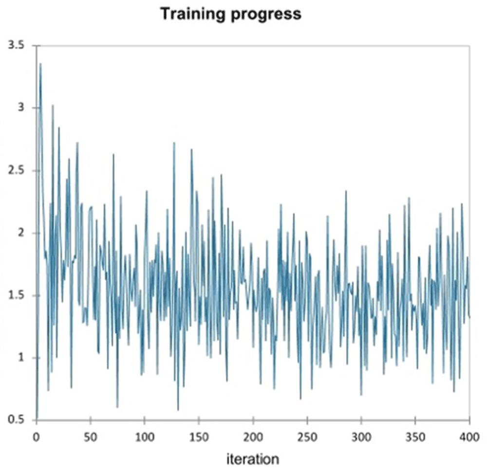
Figure 5. SOM training progress graph.
The chart in Figure 6 below shows a major output of the SOM, which groups the data set into a number of differently-characterised clusters, and shows which cluster, or node, is the best or closest match for each individual multi-dimensional observation (or here, each full bar) in the data set. For example, Figure 6 shows that the best matched node for observation 12 (bar 12) is node 9, and the best matched node for bar 20 is node 1. The following figures will explain how the remaining outputs of an SOM in XLSTAT give information about the characteristics of these different clusters or nodes, each of which roughly correspond to a broad approach to the distribution of beat lengths.
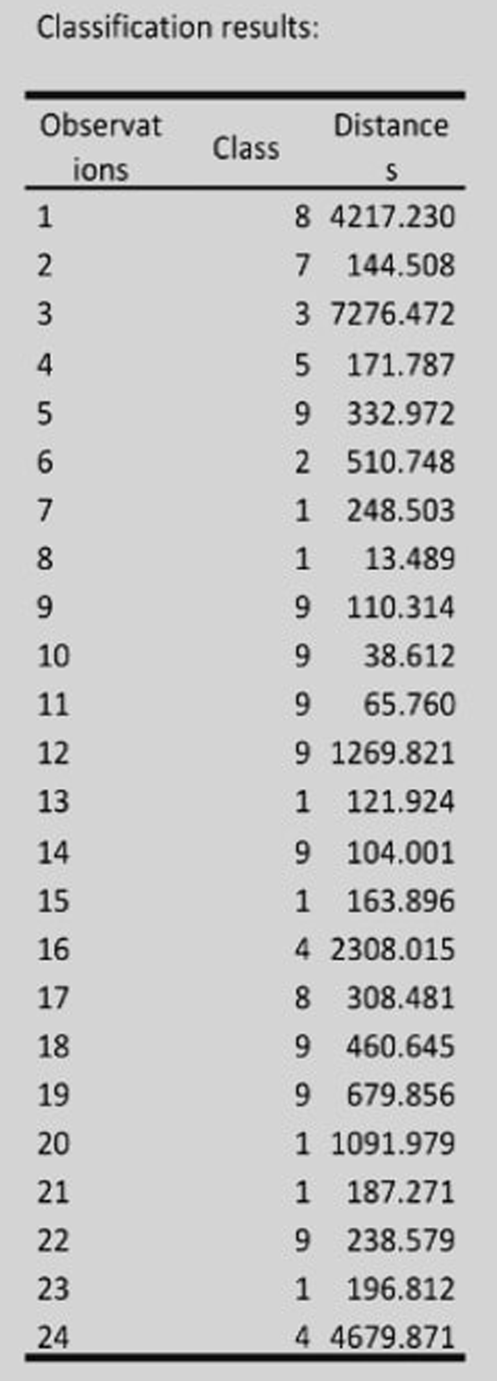
Figure 6. XLSTAT output from SOM, showing the best-matched node for each bar.
XLSTAT outputs three visualisations each time an SOM is run. Firstly, the codes plot, shown in Figure 7 (this example and those in Figure 8 and Figure 9 showing results from Participant 4’s first recording of ‘Bethena’), comprises a sequence of fan diagrams and indicates the weighting of variables in each of the different pattern-type clusters identified by the SOM. XLSTAT was set up to output 9 clusters, or nodes, each time I ran the process on any of the 24-item, three-dimensional data sets I analysed. This means that each of the resulting visualisations contains nine nodes (shown as stacked circles), each representing some information about one of these pattern types. Somewhat counter-intuitively, the nodes in all the visualisations produced by XLSTAT are numbered as follows:
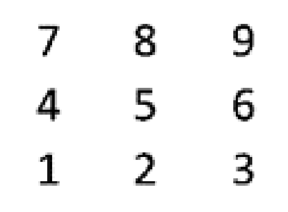
Figure 7. SOM numbers layout.
Furthermore, these XLSTAT visualisations are initially all a little counter-intuitive to look at because a larger number in this data set actually means a higher bpm, which means a shorter or ‘smaller’ sounding beat; to interpret the graphic outputs in terms of longer and shorter notes or beats, the proportions have to be inverted. So in this example from Participant 4 (Figure 7), for instance, the top right circle (node 9) shows what appears to be a proportionally shorter beat 2, but actually represents a longer beat 2. Similarly, in the lefthand circle on the middle row (node 4), beat 2 is proportionally minimal enough to not be visually represented – which actually means the bpm value is lower, and therefore that this pattern-type is characterised by beat 2 being longer than the other beats. In the righthand circle on the middle row, the three beats are almost equal lengths.
The second visualisation produced is the counts plot (Figure 8), where the nodes are numbered in the same way as above. The red and yellow circles indicate which of the clusters has the most best-matched observations from the input data set (pale yellow being the most and red being the least). In this case one of the most frequently-best-matched nodes was node 9 (top right), which therefore represents one of the most common types of pattern in this performance from Participant 4. Referring back to the codes plot, it can be ascertained that this frequently-occuring pattern is characterised by a slightly shorter beat 1 and a longer beat 2.
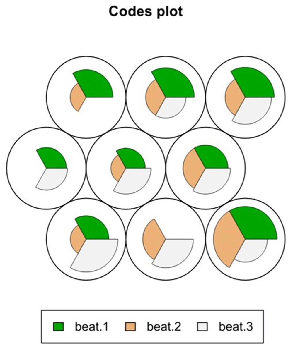
Figure 8. XLSTAT codes plot for SOM, using beat tempo data from Participant 4, ‘Bethena’ recording 1.
Lastly, the variables influence plot (Figure 9) shows the overall influence of each variable (beat 1, 2, or 3) across each of the clusters of pattern-type identified by the SOM. Like the codes plot, this graphic must be read in conjunction with the counts plot because the nine nodes are not weighted equally. Again, it is a little counter-intuitive to look at because a cooler colour temperature means a low number, but in this case a low number means a slower and therefore a longer or more prominent/emphasised beat. So, the large number of green or blue circles for the beat 2 variable in almost every cluster in this example actually indicates that beat 2 was longer in almost every cluster identified by the SOM. This is confirmed by the codes plot, where beat 2 is visually very small (and therefore numerically low and temporally longer) in almost every cluster in this performance by Participant 4. Referring again to node 9 (top right in each case), we can see that beat 2 is longest in node 9 (having a lower colour temperature on the heatmap). Once again inverting the values as interpreted by XLSTAT, a warmer colour temperature in these heatmaps indicates a faster/shorter or less emphasised beat. Cross-referencing with the counts plot, which shows that the most significant nodes for this sample are 1, 5, 8 and 9 (bottom left, centre, and top centre and right), it is clear that beat 2 is longest in all of the most commonly-occurring patterns, which shows that this performance was generally characterised by a tendency towards elongating the second beat.
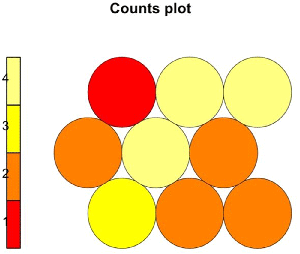
Figure 9. counts plot for P4B1 SOM.
Figure 10 below shows some outputs from the SOM that indicate differences between patterns across types of recording. In the top row of Figure 10, two patterns with a longer beat 2 are the most frequently occuring; this output comes from Participant 2’s second recording of ‘Bethena’. Meanwhile, the second row shows Participant 5’s first recording of ‘Bethena’, in which the distribution of pattern types is much more heterogenous, with the most commonly-occurring patterns characterised by a shorter beat 1, followed by a longer beat 1 and a longer beat 2.
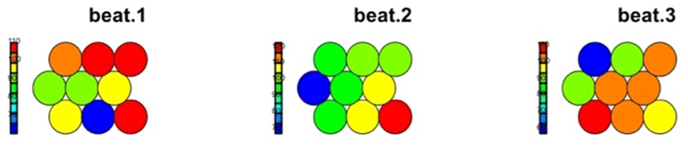
Figure 10. variables influence plot for P4B1 SOM.
Figure 11’s top row represents the most common pattern types in the ‘control sample’ recording of ‘Valse’, in which there are multiple frequently-occurring pattern types, seemingly characterised by a much longer beat 1 or a longer beat 2. On the second row, the SOM results from Alice Sara Ott’s recording of ‘Valse’ conversely indicate a performance with much less variety of pattern type, in which far and away the most common is a shape which looks almost even but appears to have a slightly shorter beat 1 and 2.
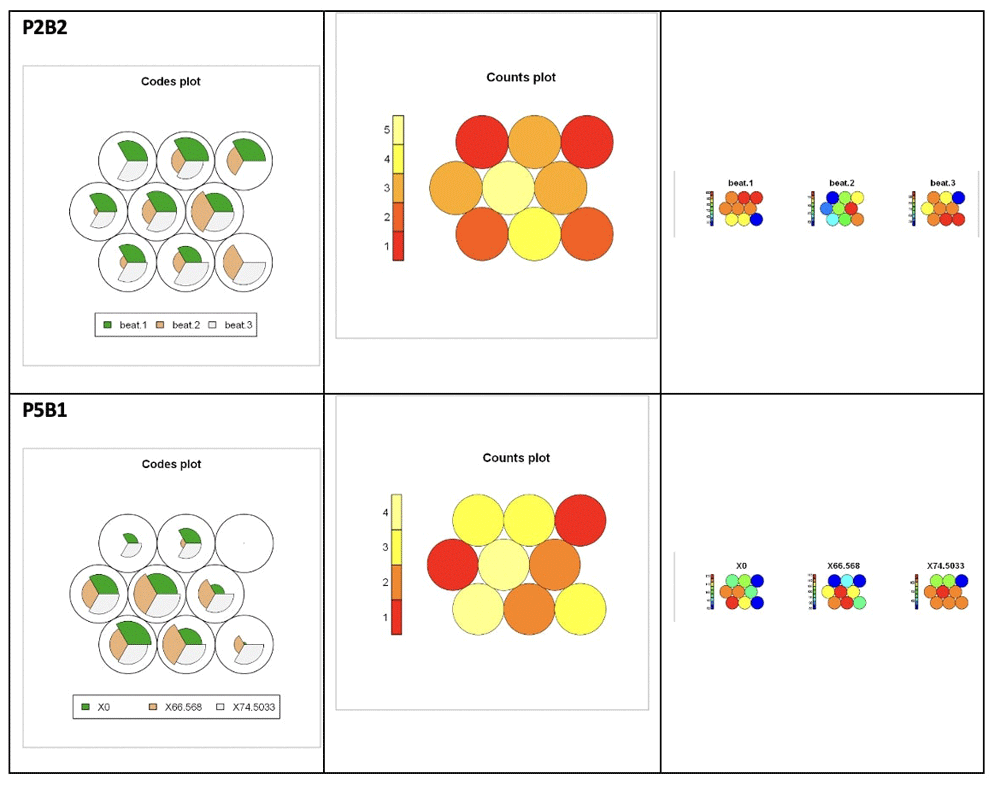
Figure 11. SOM outputs for P2B2 and P5B1 recordings of ‘Bethena’.
These and the other SOM outputs shown in Appendices 1 and 2 indicate that there are different tendencies across the collected sample of recordings (McGinn, 2022). In order to make more sense of the visible differences between recordings, we can take a closer look at the distribution of pattern-types across the set using the bpm data.
Broader analysis of results
The SOM results can point to the most common types of pattern for an individual bar in a given performance, and can also indicate the overall influence of a given variable, like ‘beat 1’, in a performance overall. The following are some observations that emerged from the collected results. Appendices 1 and 2 contain tables showing the codes plot, counts plot and variable influence plot (and, therefore, the most commonly occurring patterns of intra-bar beat-length distribution) for every recording of ‘Bethena’ and ‘Valse’.
The SOM output graphics immediately illustrated the fact that markedly different shapes characterised different recordings, and a broader look suggested that an elongated beat two was more common in performances of music box performances of ‘Bethena’ in general by comparison with music box performances of ‘Valse’. In the piano recordings, however, both sets showed the same tendencies of emphasis: in ‘Valse, two of the pianists emphasised beat 1 the most, and one emphasised beat 2 the most; this was also the case in ‘Bethena’. As a whole, the SOM results illustrated that, in the music box recordings, ‘Valse’ was generally characterised by a stronger beat 1 and ‘Bethena’ by a stronger beat 2 or 3. Closer inspection, using the manually selected threshold of 10bpm, supported this observation – as well as confirming in more detail the different tendencies across the two repertoire samples. We will consider these patterns in greater detail shortly by looking at the bpm data directly.
This trend of different emphasis points across music box recordings of the two different extracts was unexpected, and is interesting because it suggests not only that something about the perceived character of the music might incite some players to apply different kinds of physical energy when approaching each piece, but that such differences might be preserved and perceptible as distinct patterns in a mechanical performance. So, the results suggest that it is possible for idiomatic performances to be given using mechanical instruments. This is further reinforced by the fact that different tendencies across different players were also clearly visible. The extent to which additional meanings might already be extrapolated from these preliminary findings is debatable, but it is clear from the phrase-arching section and from some voluntary comments made by participants that some of them fully intended to create ‘expressive’ performances or to deliberately mirror conventions like end-slowing.
According to the Table 4–Table 10, based on onset bpm data, the differential trend between ‘Bethena’ and ‘Valse’ was preserved in the metronome-following ‘control samples’, which (as discussed previously) represented a highly imperfect solution, but which could nevertheless pose a problem for the suggestion that different patterns of beat elongation might be the result of expressive choices. As discussed earlier, attempting to follow a metronome with a mechanical instrument is ineffective and does not result in the most ‘regular’ performance. This approach may have disrupted or minimised some tendencies that might have emerged without the condition of trying to follow a metronome, but the control samples still showed evidence of phrase-arching and a trend towards emphasising different beats of the bar in the two different pieces. The question of whether the programmed card music affected these results is therefore yet to be fully resolved; Figure 12, below, shows the first bars of the ‘Bethena’ (top) and ‘Valse’ music rolls. Although it is not impossible that some characteristic of the music roll could contribute to the temporal output, it seems unlikely that a tendency towards a stretched-out beat 2 would consistently materialise throughout the extract in the programming of ‘Bethena’ but not of ‘Valse’, since the ‘left hand’ accompaniment figure in both extracts is extremely texturally similar. Figure 14 show the distribution of bars with a longer first, second, or third beat across the whole extract in each recording.
Table 4. Bars with a longer beat 1 (yellow) in ‘Bethena’.
| 1 | 2 | 3 | 4 | 5 | 6 | 7 | 8 | 9 | 10 | 11 | 12 | 13 | 14 | 15 | 16 | 17 | 18 | 19 | 20 | 21 | 22 | 23 | 24 | |
| P1 | | | | | | | | | | | | | | | | | | | | | | | | | 3 |
| P12 | | | | | | | | | | | | | | | | | | | | | | | | | 1 |
| P2 | | | | | | | | | | | | | | | | | | | | | | | | | 2 |
| P22 | | | | | | | | | | | | | | | | | | | | | | | | | 5 |
| P3 | | | | | | | | | | | | | | | | | | | | | | | | | 4 |
| P32 | | | | | | | | | | | | | | | | | | | | | | | | | 1 |
| P4 | | | | | | | | | | | | | | | | | | | | | | | | | 4 |
| P42 | | | | | | | | | | | | | | | | | | | | | | | | | 3 |
| P5 | | | | | | | | | | | | | | | | | | | | | | | | | 4 |
| P52 | | | | | | | | | | | | | | | | | | | | | | | | | 7 |
| P6 | | | | | | | | | | | | | | | | | | | | | | | | | 0 |
| P62 | | | | | | | | | | | | | | | | | | | | | | | | | 3 |
| CS | | | | | | | | | | | | | | | | | | | | | | | | | 6 |
| CS2 | | | | | | | | | | | | | | | | | | | | | | | | | 1 |
| JS | | | | | | | | | | | | | | | | | | | | | | | | | 8 |
| WA | | | | | | | | | | | | | | | | | | | | | | | | | 7 |
| JR | | | | | | | | | | | | | | | | | | | | | | | | | 6 |
| | 2 | 2 | 3 | 3 | 3 | 4 | 1 | 8 | 2 | 4 | 1 | 3 | 2 | 1 | 1 | 8 | 3 | 5 | 4 | 1 | 3 | 1 | | |
Table 5. Bars with a longer beat 2 (blue) in ‘Bethena’.
| 1 | 2 | 3 | 4 | 5 | 6 | 7 | 8 | 9 | 10 | 11 | 12 | 13 | 14 | 15 | 16 | 17 | 18 | 19 | 20 | 21 | 22 | 23 | 24 | |
| P1 | | | | | | | | | | | | | | | | | | | | | | | | | 2 |
| P12 | | | | | | | | | | | | | | | | | | | | | | | | | 3 |
| P2 | | | | | | | | | | | | | | | | | | | | | | | | | 2 |
| P22 | | | | | | | | | | | | | | | | | | | | | | | | | 4 |
| P3 | | | | | | | | | | | | | | | | | | | | | | | | | 7 |
| P32 | | | | | | | | | | | | | | | | | | | | | | | | | 3 |
| P4 | | | | | | | | | | | | | | | | | | | | | | | | | 6 |
| P42 | | | | | | | | | | | | | | | | | | | | | | | | | 9 |
| P5 | | | | | | | | | | | | | | | | | | | | | | | | | 8 |
| P52 | | | | | | | | | | | | | | | | | | | | | | | | | 4 |
| P6 | | | | | | | | | | | | | | | | | | | | | | | | | 0 |
| P62 | | | | | | | | | | | | | | | | | | | | | | | | | 3 |
| CS | | | | | | | | | | | | | | | | | | | | | | | | | 4 |
| CS2 | | | | | | | | | | | | | | | | | | | | | | | | | 1 |
| JS | | | | | | | | | | | | | | | | | | | | | | | | | 6 |
| WA | | | | | | | | | | | | | | | | | | | | | | | | | 2 |
| JR | | | | | | | | | | | | | | | | | | | | | | | | | 11 |
| | 2 | 4 | 5 | 4 | 2 | 6 | 5 | 1 | 2 | 6 | 2 | 4 | 3 | 3 | 3 | 3 | 2 | 0 | 5 | 4 | 5 | 3 | | |
Table 6. Bars with a longer beat 3 (red) in ‘Bethena’.
| 1 | 2 | 3 | 4 | 5 | 6 | 7 | 8 | 9 | 10 | 11 | 12 | 13 | 14 | 15 | 16 | 17 | 18 | 19 | 20 | 21 | 22 | 23 | 24 | |
| P1 | | | | | | | | | | | | | | | | | | | | | | | | | 0 |
| P12 | | | | | | | | | | | | | | | | | | | | | | | | | 1 |
| P2 | | | | | | | | | | | | | | | | | | | | | | | | | 5 |
| P22 | | | | | | | | | | | | | | | | | | | | | | | | | 6 |
| P3 | | | | | | | | | | | | | | | | | | | | | | | | | 1 |
| P32 | | | | | | | | | | | | | | | | | | | | | | | | | 4 |
| P4 | | | | | | | | | | | | | | | | | | | | | | | | | 7 |
| P42 | | | | | | | | | | | | | | | | | | | | | | | | | 5 |
| P5 | | | | | | | | | | | | | | | | | | | | | | | | | 7 |
| P52 | | | | | | | | | | | | | | | | | | | | | | | | | 9 |
| P6 | | | | | | | | | | | | | | | | | | | | | | | | | 0 |
| P62 | | | | | | | | | | | | | | | | | | | | | | | | | 0 |
| CS | | | | | | | | | | | | | | | | | | | | | | | | | 6 |
| CS2 | | | | | | | | | | | | | | | | | | | | | | | | | 5 |
| JS | | | | | | | | | | | | | | | | | | | | | | | | | 2 |
| WA | | | | | | | | | | | | | | | | | | | | | | | | | 3 |
| JR | | | | | | | | | | | | | | | | | | | | | | | | | 1 |
| | 2 | 3 | 4 | 3 | 6 | 0 | 3 | 2 | 2 | 1 | 3 | 1 | 2 | 2 | 6 | 0 | 4 | 6 | 3 | 4 | 2 | 3 | | |
Table 7. bars with a longer beat 1 (orange) in ‘Valse’.
| 1 | 2 | 3 | 4 | 5 | 6 | 7 | 8 | 9 | 10 | 11 | 12 | 13 | 14 | 15 | 16 | 17 | 18 | 19 | 20 | 21 | 22 | 23 | 24 | |
| P1V | | | | | | | | | | | | | | | | | | | | | | | | | 3 |
| P1V2 | | | | | | | | | | | | | | | | | | | | | | | | | 2 |
| P2V | | | | | | | | | | | | | | | | | | | | | | | | | 6 |
| P2V2 | | | | | | | | | | | | | | | | | | | | | | | | | 3 |
| P3V | | | | | | | | | | | | | | | | | | | | | | | | | 1 |
| P3V2 | | | | | | | | | | | | | | | | | | | | | | | | | 4 |
| P4V | | | | | | | | | | | | | | | | | | | | | | | | | 7 |
| P4V2 | | | | | | | | | | | | | | | | | | | | | | | | | 4 |
| P5V | | | | | | | | | | | | | | | | | | | | | | | | | 6 |
| P5V2 | | | | | | | | | | | | | | | | | | | | | | | | | 7 |
| P6V | | | | | | | | | | | | | | | | | | | | | | | | | 2 |
| P6V2 | | | | | | | | | | | | | | | | | | | | | | | | | 3 |
| CSV | | | | | | | | | | | | | | | | | | | | | | | | | 4 |
| CSV2 | | | | | | | | | | | | | | | | | | | | | | | | | 2 |
| ASO | | | | | | | | | | | | | | | | | | | | | | | | | 6 |
| DTS | | | | | | | | | | | | | | | | | | | | | | | | | 5 |
| AR | | | | | | | | | | | | | | | | | | | | | | | | | 8 |
| | 3 | 3 | 6 | 3 | 3 | 3 | 2 | 7 | 4 | 2 | 2 | 4 | 2 | 1 | | 7 | 3 | 6 | 2 | 4 | 5 | 1 | | |
Table 8. bars with a longer beat 2 (purple) in ‘Valse’.
| 1 | 2 | 3 | 4 | 5 | 6 | 7 | 8 | 9 | 10 | 11 | 12 | 13 | 14 | 15 | 16 | 17 | 18 | 19 | 20 | 21 | 22 | 23 | 24 | |
| P1V | | | | | | | | | | | | | | | | | | | | | | | | | 2 |
| P1V2 | | | | | | | | | | | | | | | | | | | | | | | | | 2 |
| P2V | | | | | | | | | | | | | | | | | | | | | | | | | 2 |
| P2V2 | | | | | | | | | | | | | | | | | | | | | | | | | 2 |
| P3V | | | | | | | | | | | | | | | | | | | | | | | | | 1 |
| P3V2 | | | | | | | | | | | | | | | | | | | | | | | | | 4 |
| P4V | | | | | | | | | | | | | | | | | | | | | | | | | 2 |
| P4V2 | | | | | | | | | | | | | | | | | | | | | | | | | 7 |
| P5V | | | | | | | | | | | | | | | | | | | | | | | | | 5 |
| P5V2 | | | | | | | | | | | | | | | | | | | | | | | | | 4 |
| P6V | | | | | | | | | | | | | | | | | | | | | | | | | 1 |
| P6V2 | | | | | | | | | | | | | | | | | | | | | | | | | 4 |
| CSV | | | | | | | | | | | | | | | | | | | | | | | | | 2 |
| CSV2 | | | | | | | | | | | | | | | | | | | | | | | | | 3 |
| ASO | | | | | | | | | | | | | | | | | | | | | | | | | 3 |
| DTS | | | | | | | | | | | | | | | | | | | | | | | | | 11 |
| AR | | | | | | | | | | | | | | | | | | | | | | | | | 3 |
| | 5 | 6 | 2 | 3 | 1 | 2 | 2 | 1 | 3 | 1 | 3 | 3 | 2 | 3 | | 2 | 2 | 5 | 3 | 2 | 7 | 0 | | |
Table 9. bars with a longer beat 3 (green) in ‘Valse’.
| 1 | 2 | 3 | 4 | 5 | 6 | 7 | 8 | 9 | 10 | 11 | 12 | 13 | 14 | 15 | 16 | 17 | 18 | 19 | 20 | 21 | 22 | 23 | 24 | |
| P1V | | | | | | | | | | | | | | | | | | | | | | | | | 4 |
| P1V2 | | | | | | | | | | | | | | | | | | | | | | | | | 2 |
| P2V | | | | | | | | | | | | | | | | | | | | | | | | | 3 |
| P2V2 | | | | | | | | | | | | | | | | | | | | | | | | | 3 |
| P3V | | | | | | | | | | | | | | | | | | | | | | | | | 0 |
| P3V2 | | | | | | | | | | | | | | | | | | | | | | | | | 1 |
| P4V | | | | | | | | | | | | | | | | | | | | | | | | | 2 |
| P4V2 | | | | | | | | | | | | | | | | | | | | | | | | | 5 |
| P5V | | | | | | | | | | | | | | | | | | | | | | | | | 4 |
| P5V2 | | | | | | | | | | | | | | | | | | | | | | | | | 6 |
| P6V | | | | | | | | | | | | | | | | | | | | | | | | | 0 |
| P6V2 | | | | | | | | | | | | | | | | | | | | | | | | | 2 |
| CSV | | | | | | | | | | | | | | | | | | | | | | | | | 1 |
| CSV2 | | | | | | | | | | | | | | | | | | | | | | | | | 4 |
| ASO | | | | | | | | | | | | | | | | | | | | | | | | | 5 |
| DTS | | | | | | | | | | | | | | | | | | | | | | | | | 0 |
| AR | | | | | | | | | | | | | | | | | | | | | | | | | 4 |
| | 2 | 2 | 4 | 1 | 1 | 2 | 4 | 0 | 0 | 1 | 1 | 0 | 1 | 5 | | 1 | 5 | 3 | 2 | 2 | 1 | 8 | | |
Table 10. table showing each player’s most-emphasised beats in total across both performances of ‘Valse and ‘Bethena’.
| ‘Bethena’ | ‘Valse’ |
| beat | 1 | 2 | 3 | 1 | 2 | 3 |
| P1 | 4 | 5 | 1 | 5 | 4 | 6 |
| P2 | 7 | 6 | 11 | 9 | 4 | 6 |
| P3 | 5 | 10 | 5 | 5 | 5 | 1 |
| P4 | 7 | 15 | 12 | 11 | 9 | 7 |
| P5 | 11 | 12 | 16 | 13 | 9 | 10 |
| P6 | 3 | 3 | 0 | 5 | 5 | 2 |
| CS | 7 | 5 | 11 | 6 | 5 | 5 |
| JS | 8 | 6 | 2 | |
| WA | 7 | 2 | 3 | |
| JR | 6 | 11 | 6 | |
| ASO | | 6 | 3 | 5 |
| DTS | | 5 | 11 | 0 |
| AR | | 8 | 3 | 4 |
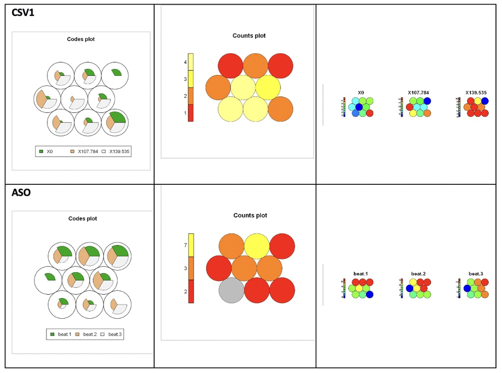
Figure 12. SOM outputs for control sample and Alice Sara Ott recordings of ‘Valse’.
Table 4–Table 9 and the overview in Figure 13 use a threshold that considers a bar as having a ‘longer beat two’ if the second beat is at least 10bpm longer than the shortest beat, and is also longer than the other beat by any amount. This risks including some bars where, for example, beats one and two are almost the same and beat three is short, but it also excludes some bars where beat two is the longest beat but by less than the threshold of 10 bpm (for example, 8 or even 9.9 bpm). The data could be measured in a number of different ways but for initial comparative purposes this threshold was selected, and is complemented by the additional use of the SOM process. Since the same measure is used across all recordings, the primary outcome – that there are differences between performances (Participant 3 showing different tendencies compared with Participant 4), instruments (music box and piano recordings yielding different patterns), and pieces (different trends across recordings of ‘Bethena’ and of ‘Valse’) – should not be affected by the limitations of this threshold. Moreover, these conclusions are supported by the SOM outputs, which do not factor in the concept of bpm and which use different measures of similarity and difference to group the data points.
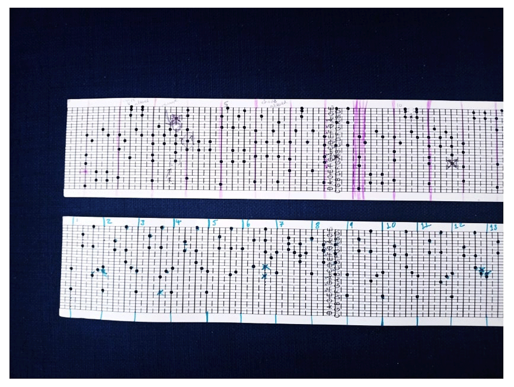
Figure 13. card-roll programmed music for ‘Bethena’ (top) and ‘Valse’ (below).
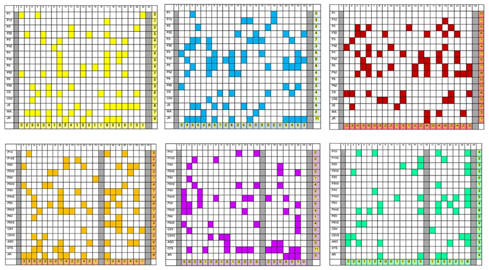
Figure 14. overview distribution of beat 1, 2 and 3 emphasis in all performances of ‘Bethena’ (top row, L-R) and ‘Valse’ (bottom row, L-R).
Some points of agreement emerge around cadences or conventional points of emphasis or slowing (such elongating as the first beat of a new phrase/section), but there is still a considerable amount of heterogeneity in the distribution of these patterns, therefore implying that the prevalence of this pattern was not (or at least not only) a feature of how the music was programmed in the card roll. The first bar is always blank because the nature of the onset calculation (duration from previous beat) means that the bpm value for beat 1 of bar 1 is always 0, thus making other values for this bar less proportionally meaningful. The last bar is always blank because the third beat of this bar in the score is a rest, so there is no beat 3 data for comparison, and in ‘Valse’ bar 16 is also blank because there is no onset on the second beat of this bar.
In both ‘Bethena’ and ‘Valse’, bars 9 and 17 are strong points of correlation for beat 1 elongation across music box and piano recordings. These points are equivalent to the first beat of a new section or phrase and therefore might conventionally be emphasised through duration, dynamic or articulation in other kinds of performance. Participants 4 and 5, both of whom showed a strong tendency to mirror European classical performance conventions like end-slowing and global tempo differentiation between (sub)sections, correlated quite strongly with the prepared recordings by pianists in terms of where they elongated beat 1. However, the music box samples also showed concentrations of beat 1 elongation at points where the piano recordings did not. In ‘Valse’, bar 19 was the highest point of agreement for beat 1 elongation across the music box samples, but none of the pianists significantly elongated beat 1 in this bar.
Some of the places where longer-second-beat bars occur also coincide with structural points in the music, although the distribution is more evenly spread compared with the more concentrated points of agreement in beat 1 elongation. The points of strongest agreement for beat 2 elongation across music box recordings are bar 7 and 11 (approaching an imperfect cadence). While some of the strongest points for beat 1 elongation are shared between recordings by pianists and music box players, none of the piano recordings showed an elongated beat 2 in bar 7; similarly, the strongest points of agreement regarding the elongation of beat 3 in the music box recordings of ‘Bethena’ were not apparent in the piano recordings. That there is a certain amount of correlation between different recordings by the same participant in some cases (Participant 4, Participant 5) further suggests that although elongating beat 2 (or beat 3 or beat 1, though the latter is perhaps most likely to be deliberate) might not necessarily be a conscious decision, it could be indicative of some other choice or intention of a music box player in relation to some part of the music.
In terms of beat 3 elongation, the comparatively low numbers in the piano recordings (regardless of the repertoire) may seem to contradict the findings of the phrase-arching/end-slowing tables. This partly pertains to the way that the threshold is applied and the way in which the player approaches structural tempo changes like end-slowing. In the pianist examples, the performers were more likely to gradually reduce the tempo change in phrase arching so that there is not necessarily a difference of 10 bpm or more between beat 3 and other beats of the bar towards the end of a phrase. Thus, a longer, more controlled rallentando is less likely to produce bpm data where one beat of the bar appears significantly longer than those next to it. The tendency to emphasise beat one, beat two, and beat three was notably high across the music box recordings by Participants 4 and 5. Both these participants reflected other European classical performance conventions. As such, the fact that the piano recordings yielded slightly lower values for beat 3 elongation overall suggests that one important difference between ‘idiomatic windows’ (de Souza, 2017), in terms of timing, of the hand-cranked music box and the piano is how finely a player (at least, one who has not played the instrument a great deal, since this could also be a significant factor) can control the rate of tempo change and degree of tempo fluctuation across a phrase or passage.
In ‘Bethena, the player who most frequently emphasised beat 1 in a bar was Participant 5 (11 times), followed by pianist Janice Scroggins (eight times); in ‘Valse’, it was again Participant 5 (13 times), followed by Participants 4 (11 times) and 2 (nine times). In ‘Bethena’ the least frequent emphasisers of beat 1 were Participants 6 (three times) and 1 (four times). In both cases, Participants 4 (15 times in ‘Bethena’, nine times in ‘Valse’) and 5 (12 times in ‘Bethena’, nine times in ‘Valse’), among the music box players, were the ones to most frequently elongate beat 2, along with one pianist in each case (Dang Thai Son, 11 times in ‘Valse’, and Joshua Rifkin, 11 times in ‘Bethena’). Participants 1, 2 and 6, as well as the ‘control samples’ recorded with a metronome, were less or much less likely to do so. Interestingly, the players who least frequently emphasised beat 2 the most in a bar were almost all pianists – in ‘Valse’, Alice Sara Ott (three times) and Artur Rubinstein (three times); in ‘Bethena’, William Appling (twice) and Participant 6 (three times). The players who most frequently emphasised beat 3 in ‘Bethena’ were Participant 5 (16 times), Participant 2 (11 times), and the ‘control’ sample (11 times); in ‘Valse’, the most frequent emphasisers of beat 3 were Participants 5 (10 times), 4 (seven times), and 1 (six times). The least frequent emphasis on beat 3 was demonstrated by pianist Dang Thai Son (0 times), followed by Participants 3 (once) and 6 (twice). As mentioned elsewhere, the overall disparity between music box and piano recordings in terms of beat-three-emphasis may relate in part to the greater capacity of the piano to allow longer, more finely gradated or more easily controlled periods of slowing down or speeding up, so that there may be less likelihood of a significant drop or leap in tempo within a single bar in the context of end-slowing. Participants 2, 4 and 5, as shown in the previous section, were more likely to employ end-slowing or phrase-arching, while Participants 3 and 6 were less likely to do so; Participant 1 and the control samples were somewhere in the middle. Participants 4 and 5 were more likely to differentiate between beat lengths in different bars in general, while Participant 6, for example, showed less tendency to vary beat lengths. In the samples of piano recordings for each piece, one of the three pianists in each case showed a significantly greater tendency than the others to elongate beat 2.
In bars 8, 11, 13, and 22 of ‘Bethena’, Participant 4 elongated beat 2 in both their first and second renditions of the piece. At each of these these points, pianist Joshua Rifkin also elongates beat 2 (and Participant 5 also elongates beat 2 in bars 8, 11 and 22 in one of their recordings). This does not necessarily demonstrate that these patterns are commensurate with any interpretive strategy, as more detailed investigation would be needed to measure this. Tools like Principal Components Analysis could be considered, but might not be so effective when making comparisons across very different instruments in this way, since the music box’s handle mechanism and tendency to produce some unintended irregularities could create seemingly anomalous patterns that might disrupt a broader recognition of common intentions in phrasing. However, for the time being it is at least notable that these patterns of beat-2 elongation are repeated across different music box performances by participants who demonstrated intentionality in relation to conventions like phrase-arching and sectional tempo variation, and are also mirrored in a prepared performance by a classical pianist. In the ‘Bethena’ music box tables there is a higher occurrence of beat 2 and beat 3 elongation overall, but less concentration or consensus at certain points by comparison with beat 1 elongation. In ‘Valse’ overall, there was both a strong tendency to emphasise beat 1 and a relatively weaker tendency to emphasise either beat 2 or beat 3. Although one bar in the middle of ‘Valse’ does not yield any useable onset tempo data because it has a rest on the second beat of the bar, the extent to which ‘Bethena’ sees a higher prevalence of beat 2 and 3 elongation seems to be significant even taking this into account. If we add the value of more (say, 8) than the highest number of beat-2-elongations (6) found in one bar in ‘Bethena’ to the total number of beat-2-elongations in ‘Valse’, the total is still 66 to ‘Bethena’’s 75.
As is evident in Table 10 and Table 11, there is a clear trend in ‘Bethena’ towards beats two and three and less tendency to emphasise beat one the most, whereas in ‘Valse there is more of a trend towards beat one and a less concentrated tendency to emphasise beats two and three the most. Participants 3 and 6 still leaned more towards emphasising the first two beats of the bar more than the third in this extract, although there was not necessarily a single most-elongated beat as in some other cases. The small sample of piano recordings show an overall trend in most-frequent emphasis that is essentially the same across both extracts – in each case the majority of performances tend to emphasise beat one, with one player emphasising beat two, and none emphasising beat three.
Table 11. table showing most-emphasised beats in each (first and second) individual music box performance of ‘Valse and ‘Bethena’.
| ‘Bethena’ | ‘Valse’ |
| beat | 1 | 2 | 3 | 1 | 2 | 3 |
| P1 | 3 | 2 | 0 | 3 | 2 | 4 |
| P1 2 | 1 | 3 | 1 | 2 | 2 | 2 |
| P2 | 2 | 2 | 5 | 6 | 3 | 3 |
| P2 2 | 5 | 4 | 6 | 3 | 2 | 3 |
| P3 | 4 | 7 | 1 | 1 | 1 | 0 |
| P3 2 | 1 | 3 | 4 | 4 | 4 | 1 |
| P4 | 4 | 6 | 7 | 7 | 2 | 2 |
| P4 2 | 3 | 9 | 5 | 4 | 7 | 5 |
| P5 | 4 | 8 | 7 | 6 | 5 | 4 |
| P5 2 | 7 | 4 | 9 | 7 | 4 | 6 |
| P6 | 0 | 0 | 0 | 2 | 1 | 0 |
| P6 2 | 3 | 3 | 0 | 3 | 4 | 2 |
| CS | 6 | 4 | 6 | 4 | 2 | 1 |
| CS 2 | 1 | 1 | 5 | 2 | 3 | 4 |
The SOM analyses showed that music box performances were often more heterogenous in terms of number of most common pattern types than the highly-prepared piano versions. However, this heterogeneity often decresed with a second rendition of the same piece, suggesting that in part it stemmed from an unfamiliarity with the instrument and the music. In keeping with this observation, the recordings by participant 1, who had played a similar music box before, were considerably and consistently homogenous across the first and second recordings of both pieces. Table 12 shows the counts plots from both of Participant 1 and Participant 2’s recordings of ‘Bethena’; the move towards homogeneity (more red and fewer yellow circles) in P2, and the consistency of homogeneity (a highly similar colour distribution) in P1 are visible. A more systematic approach would be needed to demonstrate this clearly, but it may be possible to say that a more intentionally-conventional, prepared performance appears to also be more associated with a stronger concentration of a smaller number of types of pattern. In a number of cases here, between two non-prepared participant performances, the second rendition tends towards a greater concentration of a smaller number of pattern types. Participant 2’s recordings suggest that it is possible to play idiomatically or expressively on a hand-cranked instrument, because they imply a qualitative difference in result between turning the handle with little idea of what it will be like to play the piece in question and turning the handle with a clearer idea of what it will be like to play that piece. Contrastingly, Participant 1’s two recordings are extremely consistent in terms of high counts plot homogeneity. This in turn may have resulted in part from the factor of Participant 1 having previously played a hand-cranked music box, while Participant 2 had not.
Preliminary conclusions
Based on the investigations described above, it seems that idiomatic or ‘individual’ playing is possible on a hand-cranked mechanical music box. That is to say, first of all, that the outputs are far from being robotically uniform, monotonously similar or characterless. In terms of different patterns of beat-lengths, the question of whether or not these differences can be straightforwardly related to conventions of ‘expressive’ playing is a more complex one. However, the clear differences between participants, instruments, and extracts at least allow us to posit in relation to these results that 1) different players can produce ‘idiomatic’ or individually characterisable performances on a music box; 2) renditions of different pieces or repertoires played on the same music box can demonstrate certain ‘idiomatic’ tendencies in relation to each other; 3) a music box rendition produces different enough patterns from a piano rendition that certain characteristics of the former may be described as ‘idiomatic’. Moreover, If ‘expressive’ playing was understood simply as playing in which phrase-arching is used, then several of the music box recordings analysed here could be interpreted as demonstrating ‘expressive’ playing. These results indicate that different players can and do play differently using the same mechanical instrument, that music box performances may produce some slightly different results to piano ones, and that music box performances can reflect performance trends that relate to the repertoire being played as well as mirroring (if not precisely, given the greater difficulty in finely controlling changes in tempo) standard expressive conventions like phrase-arching. Table 13 gives some indication of change and continuity across two performances of the same piece by the same player, and Table 14 shows an overview of the difference in overall beat emphasis trends across the two pieces.
Table 13. table showing difference between first and second recordings (if applicable) for all music box peformances of ‘Valse and ‘Bethena’.
| B1 → B2 | V1 → V2 |
| P1 | Little change | Little change |
| P2 | Becoming more
homogenous | Becoming more
homogenous |
| P3 | More homogenous | More homogenous |
| P4 | More heterogenous | More heterogenous |
| P5 | More homogenous | More homogenous |
| P6 | Little change | More homogeous |
| CS | More heterogenous | More homogenous |
Table 14. overall beat emphasis trends in ‘Bethena’ and ‘Valse’.
| 1 | 2 | 3 |
Music box ‘Bethena’ (excluding ‘control’
samples) | 37 | 51 | 45 |
| åMusic box ‘Bethena’ (‘control’ samples) | 7 | 5 | 11 |
| Music box ‘Bethena’ (total) | 44 | 56 | 56 |
| Piano ‘Bethena’ | 21 | 19 | 6 |
| ‘Bethena’ total (music box and piano) | 65 | 75 | 62 |
Music box ‘Valse’ (excluding ‘control’
samples) | 48 | 36 | 32 |
| Music box ‘Valse’ (‘control’ samples) | 6 | 5 | 5 |
| Music box ‘Valse’ (total) | 54 | 31 | 37 |
| Piano ‘Valse’ | 19 | 17 | 9 |
| ‘Valse’ total (music box and piano) | 73 | 58 | 46 |
Not only do hand-cranked mechanical musical instruments not necessarily produce uniformly similar temporal results each time a piece is played, but also that the repertoire, the performer and other conditions (like being given a digital suggested tempo) can influence the range of outputs. Some music box performances appeared to incorporate some kind of interpretive strategy. In some cases there were perceptible consistencies between multiple recordings by one participant that could be seen to contrast with recordings produced by another participant – supporting the possibility of idiomatic styles of playing (albeit within a narrower range than more analog instruments).
The phrase arching investigations showed that a conventional shaping of phrases by slowing down at the end can be a feature of music box performances. Based on the initial SOM analyses and backed up with the bpm data, the most common patterns of most-emphasised beats in each type of sample are shown in the table below. The values in the table reflect the number of recordings characterised by this feature rather than the number of bars characterised by this feature (one recording may be characterised by more than one type of pattern).
Phrase arching or shaping resembling some kind of structural plan appeared to a significant extent, but by no means exclusively, in recordings by participants who were members of classical music performance discourse communities. Varied beat elongation occurred fairly evenly across music box recordings by participants with different musical experience. A player’s somatic responses to heard music don’t result only from formal training but also from tacit knowledge and other factors. As shown in Figure 13 above, bars with a longer beat 2 did not necessarily occur in the same places in the music across different recordings (though there were some stronger points of agreement close to structural cadences).
Many organ grinders demonstrated an active interest in creating performances that conformed to contemporary aesthetic preferences (for example, by taking care that their repertoire was up to date with the latest trends), and tacit as well as more explicitly learned knowledge of current conventions of instrumental performance could certainly have fed into this. More interesting is that, overall, these hand-cranked mechanical performances (in comparison with those by pianists) were also characterised by alternative and potentially repertoire-contingent temporal patterns. At the same time as some organ grinders would have used the flexibility afforded by their instruments to create performances that were more normative, others (as perhaps reflected in contemporary complaints that buskers were playing famous repertoire ‘wrong’) would have used that flexibility in different ways. The motivation of this research is not to argue that organ grinders were valid creative music makers because they could, after all, play ‘expressively’ according to certain dominant conventions. The aim is rather to show that by no means is every aspect of a hand-cranked mechanical performance predetermined by the machine – and to highlight that the individuality and creative potential afforded by this is a relatively unexplored domain. The patterns or approaches that may emerge as characteristic of hand-cranked mechanical renditions do not need to be dismissed as bad or necessarily to be re-evaluated as ‘good’, but can and should be recognised as part of a significant musical performance tradition.
Data availability
DANS: Expressive timing and mechanical instruments.
https://doi.org/10.17026/dans-xgy-rjhp. (McGinn, (2022))
This project contains the following underlying data:
Data file 1. (Appendix 1: PDF showing SOM results from onsets data from ‘Bethena’ music box recordings.)
Data file 2. (Appendix 2: PDF showing SOM results from onsets data from ‘Valse’ music box recordings.)
Data file 3. (Control sample, first recording of ‘Bethena’ with metronome.)
Data file 4. (Control sample, second recording of ‘Bethena’ with metronome.)
Data file 5. (Control sample, first recording of ‘Valse’ with metronome.)
Data file 6. (Control sample, second recording of ‘Valse’ with metronome.)
Data file 7. (Second recording of ‘Bethena’ by Participant 1.)
Data file 8. (First recording of ‘Valse’ by Participant 1.)
Data file 9. (Second recording of ‘Valse’ by Participant 1.)
Data file 10. (First recording of ‘Bethena’ by Participant 2.)
Data file 11. (Second recording of ‘Bethena’ by Participant 2.)
Data file 12. (First recording of ‘Valse’ by Participant 2.)
Data file 13. (Second recording of ‘Valse’ by Participant 2.)
Data file 14. (First recording of ‘Bethena’ by Participant 3.)
Data file 15. (Second recording of ‘Bethena’ by Participant 3.)
Data file 16. (First recording of ‘Valse’ by Participant 3.)
Data file 17. (Second recording of ‘Valse’ by Participant 3.)
Data file 18. (First recording of ‘Valse’ by Participant 4.)
Data file 19. (Second recording of ‘Valse’ by Participant 4.)
Data file 20. (Second recording of ‘Bethena’ by Participant 5.)
Data file 21. (Second recording of ‘Valse’ by Participant 5.)
Data file 22. (First recording of ‘Bethena’ by Participant 6.)
Data file 23. (Second recording of ‘Bethena’ by Participant 6.)
Data file 24. (First recording of ‘Bethena’ by Participant 1.)
Data file 25. (First recording of ‘Bethena’ by Participant 4.)
Data file 26. (Second recording of ‘Bethena’ by Participant 4.)
Data file 27. (First recording of ‘Bethena’ by Participant 5.)
Data file 28. (First recording of ‘Valse’ by Participant 5.)
Data file 29. (First recording of ‘Valse’ by Participant 6.)
Data file 30. (Second recording of ‘Valse’ by Participant 6.)
Data are available under the terms of the Creative Commons Zero “No rights reserved” data waiver (CC0 1.0 Public domain dedication).
Faculty Opinions recommendedReferences
- Accinno M:
Disabled Union veterans and the performance of martial begging. In: B. Howe, S. Jensen-Moulton, N.W Lerner, J.N Straus (Eds.) The Oxford Handbook of Music and Disability Studies. Oxford: OUP,
2015; 403–422. Publisher Full Text
- Born G:
Reinventing Audiences––Imagining Radical Musical Democracies. In: E. Buch and R. Adlington (Eds.) Finding democracy in music. Oxford and New York: Routledge, 2021; 181–203. Reference Source
- Bull A:
Class, control, and classical music. Oxford and New York: Oxford University Press, 2019. Reference Source
- Butler MJ:
Playing with something that runs. New York: Oxford University Press, 2014. Reference Source
- Clarke EF:
The perception of expressive timing in music.
Psychol Res.
1989; 51(1): 2–9. PubMed Abstract
| Publisher Full Text
- Cohen D, Greenwood B:
The buskers: History of street entertainment. Newton Abbot: David & Charles, 1981. Reference Source
- Cook N:
Beyond the Score: Music as Performance. New York: OUP,
2013. Publisher Full Text
- Cook N:
Between art and science: Music as performance.
J Br Acad.
2014; (2): 1–25. Reference Source
- De Souza J:
Music at hand: Instruments, bodies and cognition. New York: Oxford University Press, 2017. Reference Source
- Desain P, Honing H:
Tempo curves considered harmful.
Contemporary Music Review.
1993; 7(2): 123–138. Publisher Full Text
- Hudson R:
Stolen time: The history of tempo rubato. Oxford: Clarendon Press, 1994. Reference Source
- Kohonen T:
The self-organizing map.
Proceedings of the IEEE.
1990; 78(9): 1464–1480. Publisher Full Text
- Leech-Wilkinson D:
Cortot’s Berceuse.
Music Analysis.
2015; 34(3): 335–363. Publisher Full Text
- Maloney L:
Music as water: The functions of music from a utilitarian perspective.
AVANT.
2017; 8: 57–67. Publisher Full Text
- McGinn C:
Expressive timing and mechanical instruments. [dataset]. 2022. http://www.doi.org/10.17026/dans-xgy-rjhp
- Molin M:
Playing a Street Organ for the First Time. YouTube. 2017. Reference Source
- Ord-Hume AWJG:
Barrel organ: The story of the mechanical organ and its repair. London: George Allen & Unwin, 1978. Reference Source
- Roberts P:
The emergence of the magic lantern trade in nineteenth-century england. PhD thesis, University of York, 2018. Reference Source
- Schuiling F:
Notation cultures: Towards an ethnomusicology of notation.
Journal of the Royal Musical Association.
2019; 144(2): 429–458. Reference Source
- Spiro N, Gold N, Rink J:
The form of Performance: Analyzing pattern distribution in select recordings of chopin’s mazurka op. 24 no. 2.
Musicae Scientiae.
2010; 14(2): 23–55. Publisher Full Text
- Todd N:
A model of expressive timing in tonal music.
Music Perception: An Interdisciplinary Journal.
1985; 3(1): 33–57. Publisher Full Text
- Volioti G:
Expressive gesture in Grieg’s recordings of two op. 43 Lyric Pieces: An exploratory principal components analysis.
Music Performance Research.
2019; 9: 1–30. Reference Source
- Williams S:
Interpretation and performance practice in realizing Stockhausen’s Studie II.
Journal of the Royal Musical Association.
2016; 141(2): 445–481. Publisher Full Text