Plain language summary
The function of cells in many contexts require that they move and explore their surroundings. An excellent example is the movement of bacterial cells in their natural habitats, such as the forest floor or the gut. Myxococcus xanthus is a bacterial species that moves as large cell groups in search of food. In this process, they can kill and prey on other bacterial species. The study of how single cells move and prey on other bacteria has been prevented by the lack of acquisition and analysis tools able to follow the fast dynamics and to detect single bacterial cells in crowded environments. We have addressed this limitation by developing a microscopy method that enables the fast acquisition of different bacterial species over large areas. We combined this detection with an analysis method relying on artificial intelligence that is able to segment single predator and prey cells in their natural ecosystems. We implemented a technique that joins these single cells together to build a trajectory that allows researchers to characterize the collective and single cell movement of cells during bacterial predation. Finally, we have demonstrated the use of these technologies during the predation of Escherichia coli predation by Myxococcus xanthus.
Introduction
Cell motility is essential for many biological processes, such as tissue remodeling, development, or the immune response to pathogens. Cell motility in complex multi-cellular environments is controlled by external signals at the level of the organism (Devi et al., 2021; Jacobson et al., 2021), or locally by cell-cell interactions. These interactions are particularly important during predation, where cell movement needs to be halted to deploy killing strategies (Nauseef & Borregaard, 2014). A fascinating example of this coupling between motility and predation was recently reported for the process of bacterial predation by Myxoccocus xanthus (M. xanthus) (Seef et al., 2021).
M. xanthus is a gram-negative bacterium that lives in the soil. To survive in this complex ecosystem, it has developed a social lifestyle based on its capacity to move over a surface in a collective and coordinated manner (Dworkin, 1963; Zhang et al., 2012). This motility allows M. xanthus to create hunting packs able to seek prey on centimeter-scale distances, or to induce collective motion towards aggregation centers to form spore-filled fruiting bodies (Muñoz-Dorado et al., 2016). Both phenomena, predation and fruiting body formation, exceed the length scales of the single cell and arise from the strong coordinated dynamics of individual cells (Zhang et al., 2012). The process of M. xanthus predation occurs in several phases: i) exploration of the environment in search for nutrients, ii) encountering of prey, iii) progression of dense swarms to regions where prey is found, iv) killing of prey, and v) take-up of nutrients (Keane & Berleman, 2016). The occurrence of these cellular behaviors suggest that they all contribute to successful and efficient predation. However, it remains unclear how and to what extent intra- and inter-cellular behaviors affect this complex process.
Due to experimental and technical constraints, it has been challenging to study single cell behavior within the macroscopic context of bacterial predation. First, bacterial predation between M. xanthus and Escherichia coli (E. coli) is a colony-phenomenon (>1mm) that exceeds the length scales accessible with high-resolution microscopy imaging (<1µm). Therefore, it is challenging to capture an area that is large enough to provide colony-wide context while being able to resolve single bacterial cells. Second, even if a large area could be microscopically captured, M. xanthus cells aggregate into densely packed swarms during colony expansion, and E. coli cells are tightly-packed at the colony periphery or at micro-colonies or ‘islands’ (in our conditions these have a typical size of 30µm). To automatically segment cells in such dense conditions is challenging with classical methods, particularly when working with low-phototoxicity imaging conditions such as brightfield or low-intensity fluorescence. Several software packages for cell segmentation have recently become available, such as SuperSegger (Stylianidou et al., 2016), Oufti (Paintdakhi et al., 2016) and MicrobeJ (Ducret et al., 2016). However, these methods are ill suited for simultaneous segmentation of multiple bacterial species, dense bio-films and low-contrast imaging modalities (e.g., brightfield). Recently, artificial-intelligence (AI) based solutions for semantic cell segmentation of complex microbial communities were proposed that can efficiently segment and identify multiple species in millimeter-sized static images (Panigrahi et al., 2021). These methods permit the semantic segmentation of cells from static images, but do not enable the dynamic tracking of different bacterial species or collective groups with single-cell resolution.
Cells within microbial communities are constantly in motion, thus understanding the mechanisms involved in biofilm development, resource consumption, or predation requires tools able to track the movement of cells within different cell groups in space and time. For instance, M. xanthus predation of E. coli is an inherently dynamic process whereby M. xanthus cells glide towards and within E. coli colonies that disappear over time as a result of their lysis. Semantic single-cell tracking within complex microbial communities requires a method with the ability to follow cells from different species, over relevant periods of time (typically several hours), at relevant spatial scales (~ 0.1–1mm2), and with enough time resolution to identify single cell trajectories in crowded environments (typically tens of seconds). This study is based on the PhD thesis of the first named author available here (Rombouts, 2021).
Here, we present a method that addresses these challenges. First, we developed a hardware-accelerated, automated microscope to robustly image large areas of the sample (~0.4mm2), over long periods of time (>6h), and with high temporal resolution (~30s/image). Second, we applied a deep-learning approach to semantically segment single cells within densely-packed cell groups. Third, we designed a cell tracking algorithm to track single motile cells. Finally, we extracted dynamic track parameters from thousands of single-cell tracks with spatial resolution.
Methods
Bacterial cultures
The bacterial strains used in this work can be found in Underlying Table 1 (Nollmann, 2022a). E. coli cells used in predation assays were grown overnight in 10 ml Luria-Bertani (LB) medium at 32°C under agitation (200 rpm). To ensure that E. coli cells were in exponential phase after overnight growth, a 1:10 dilution of the starter culture was made in fresh LB medium and incubated for approximately four hours. M. xanthus cells were grown overnight in 10 ml Casitone Yeast Extract (CYE) rich medium as was described before (Bustamante et al., 2004) at 32°C under agitation (200 rpm), supplemented with antibiotics (Ampicillin 1 μg/ml) when necessary. Cells were harvested when the OD600 reached 0.1–0.5.
Predation assays
Bacterial predation was established in laboratory conditions by setting up a predation assay. In short, E. coli and M. xanthus cells were harvested from the LB and CYE media, respectively. Cells were concentrated by centrifugation on a tabletop centrifuge at 2100 g for 5 min at room temperature and resuspended in CF medium (10 mM MOPS (pH 7.6), 1 mM KH2PO4, 8 mM MgSO4, 0.02% (NH4)2SO4, 0.2% sodium citrate, 0.015% bacto casitone peptone). M. xanthus cells were concentrated to an OD600 of 5, E.coli cells were concentrated to an OD600 of 0.005. Cell suspensions of 1 µl were spotted at close distance of approximately 1 mm on CF 1.5% agar pads supported on a coverslip.
The agarpads used for time lapse imaging were made with ultrapure agar (UltraPure Agarose 1000, Invitrogen) to limit autofluorescence by impurities in the agar solutions. To limit any background signal during high resolution fluorescence imaging, the agar pad was made as thin as possible. In short, pads were made by pipetting 550 µl of melted agar onto a 25mm coverslip and by placing a second coverslip on the drop of agar, allowing the latter to solidify between two flat surfaces. Once the agar pad was made, the top coverslip was removed and the agar was cut to a diameter of 20 mm.
The prepared predation assays were then placed onto a layer of CF 1.5% agar in a petri dish and the petri dish was closed with parafilm to avoid agar pad evaporation and drying. Samples were incubated 24h to 48h at 32°C to allow M. xanthus cells to invade the E. coli colony.
Microscopy
Time lapse imaging was performed on a homemade fully-automated hardware-accelerated wide-field epifluorescence microscope built on a rapid automated modular microscope (RAMM) system (Applied Scientific Instrumentation). Samples were imaged using a 60x Plan-Achromat water-immersion objective (NA = 1.2, Nikon, Japan). The objective lens was mounted on a closed-loop piezoelectric stage (Nano-F100, Mad City Labs Inc. - USA). Illumination was provided by a brightfield illumination source and 2 lasers (OBIS-488 nm and Sapphire-LP-561 nm, Coherent – USA). Images were acquired using a sCMOS camera (ORCA Flash 4.0V3, Hamamatsu – Japan), with a final pixel size calibrated to 106 nm. A custom-built autofocus system was used to correct for axial drift in real-time and maintain the sample in focus. Software-controlled microscope components, including camera, stages, brightfield illumination and lasers were run using a custom-made software package developed in LabView 2015 (National Instrument).
Fast time lapse imaging
For imaging of the predation assay, the sample was covered with an imaging coverslip. The imaging coverslip was washed consecutively with acetone, Milli-Q water, 70% ethanol (v/v), and Milli-Q water, and flamed to remove any fluorescence impurities and residues. The coverslip was cooled down to room temperature and placed hermetically on the sample while avoiding bubbles between the sample and the coverslip. The sample was mounted in an open attofluor and onto the microscope for imaging. A region of interest spanning an area of approximately 0.36 mm² was selected. This large area was imaged by acquiring a mosaic patchwork of 3 by 3 fields of view (FOVs) of 2048x2048 pixels each. An overlap of 160 pixels between consecutive tiles was allowed for image registration. An imaging cycle, in which the 3-by-3 mosaic was imaged by sample displacement following a serpentine pattern, was thus made up of 9 consecutive acquisitions. For each FOV, a 3D-stack was acquired to account for sample tilt in brightfield and in the fluorescence channel of 561 nm for E. coli carrying a HU-mCherry fusion. An additional fluorescent channel was added for M. xanthus when the used strain was carrying a fluorescent protein as well. A 3D-stack was generally made up of 7–12 planes interspaced with 250–500 nm. Exposure time was set at 50 ms. The laser powers used were kept at low intensity to limit phototoxic effects on the live cells during time lapse acquisition. Imaging cycles were generally completed in 30–40 seconds and were repeated 700 times to construct an hours-long time lapse series of the mosaic area.
Treatment of fast time lapse data
The full pipeline of analysis, including script names, as well as inputs and outputs are included in underlying Table 2 (Nollmann, 2022a). To increase imaging speed, all images from one imaging cycle were pooled into one DCIMG file. First, the DCIMG files were converted to tiff files with software from Hamamatsu and sorted for each FOV, channel and time point. Tiff images of the fluorescent channel of E. coli were deconvolved with Huygens Professional version 20.04 (Scientific Volume Imaging, the Netherlands, https://svi.nl/). Deconvolved E. coli stacks were z-projected by calculating the standard deviation. 3D brightfield stacks were converted to 2D images by dividing each stack in 16 ROIs of 512x512 pixels, selecting automatically or manually the in-focus plane for each ROI and restitching the 16 ROIs. The code for calculating the in-focus brightfield image was implemented in bacto_tracker/im_straighter.m and bacto_tracker/im_straighter_manual.m. 2D brightfield and E. coli fluorescence images were used as input for a custom MATLAB script using a convolutional neural network with U-Net architecture for semantic segmentation (Ronneberger et al., 2015; Van Valen et al., 2016). Semantic segmentation was performed with five independently trained networks to converge towards a high confidence result, outputting an image with pixel values representing the pixel assignment confidence to a given class. The code for semantic segmentation was implemented in bacto_tracker/segment.m. The final database was used to independently train five networks. The trained networks can be found in bacto_tracker/Trained_networks.
Segmented images were then used to reconstruct the mosaic image by tiling the 9 images. Exact image overlap for tiling was calculated by image-based pixel-resolution cross correlation. Drift in time was corrected by aligning the mosaic images based on cross correlation calculated from segmented images of stationary E. coli microcolonies. M. xanthus segments from mosaic images were post-processed to reduce segmentation artifacts. In short, binary masks were generated from the masks by exploiting the assignment of confidence values, masks were filtered for size and finally, tortuous masks and fused masks were rejected. E. coli masks were post-processed to avoid overlap between E. coli and M. xanthus masks and filtered for size to reject isolated pixels. Drift correction cross-correlation was implemented in bacto_tracker/mosaic_drift_correction.py, tile calculation in tile_calculation.py, and mosaic assembly for bright field and fluorescence images in bacto_tracker/builds_mosaic.m.
Training data set
A large, diverse and representative training data set was constructed consisting of three sets of images: i) brightfield images, ii) their respective E. coli fluorescence images, and iii) their respective manually annotated ground truth images. The ground truth consisted of 5 classes: i) background, ii) E. coli cell body, iii) E. coli contour, iv) M. xanthus cell body, and v) M. xanthus contour.
Single cell tracking
Single cell trajectories were reconstructed with an in-house developed MATLAB pipeline. For each timepoint in the time lapse image series, pairwise tracks were constructed between cells in frame k and cells in frame k+1. Briefly, the enlarged bounding box of the cell mask in frame k was utilized to select a number of possible candidates in frame k+1. Ultimately, the optimal candidate was found by ranking the candidates with Analytical Hierarchy Processing (AHP) (Saaty, 1986) based on several parameters of the masks including cell area, cell length, and mask overlap area between the cell and its candidates. To correct for multiple assignments of a candidate, an inverse AHP approach was used in which the optimal cell from frame k was selected for the candidate of frame k+1. Finally, pairwise tracks over all timepoints were combined to form complete single cell trajectories. The code for single-cell trajectory reconstruction was implemented in bacto_tracker/tracking.m.
Results
Acquisition of high-resolution, large-scale, time course images of bacterial predation
The first step to develop and validate a method to perform single cell tracking within a complex bacterial community was to select and adapt an appropriate experimental assay. For this, we chose the predation of E. coli by M. xanthus, a well-established and well-adapted assay (Berleman et al., 2006; Panigrahi et al., 2021). We applied a few specific adaptations to this classical assay to limit the number of regions where cells cluster at extremely high-densities (e.g., colony edges) or form multi-layers. In our assay, a colony of M. xanthus was spotted at a millimeter distance from a colony of E. coli on a hard agar surface (Figure 1A) so that M. xanthus cells could reach the E. coli prey colony within a reasonable time period (~1–2 days). The optical density of E. coli was considerably reduced to prevent the formation of a sharp colony edge with high cell densities. In these conditions, E. coli grows in relatively small, intersped microcolonies typically 30µm wide with a single layer of cells (see Methods).
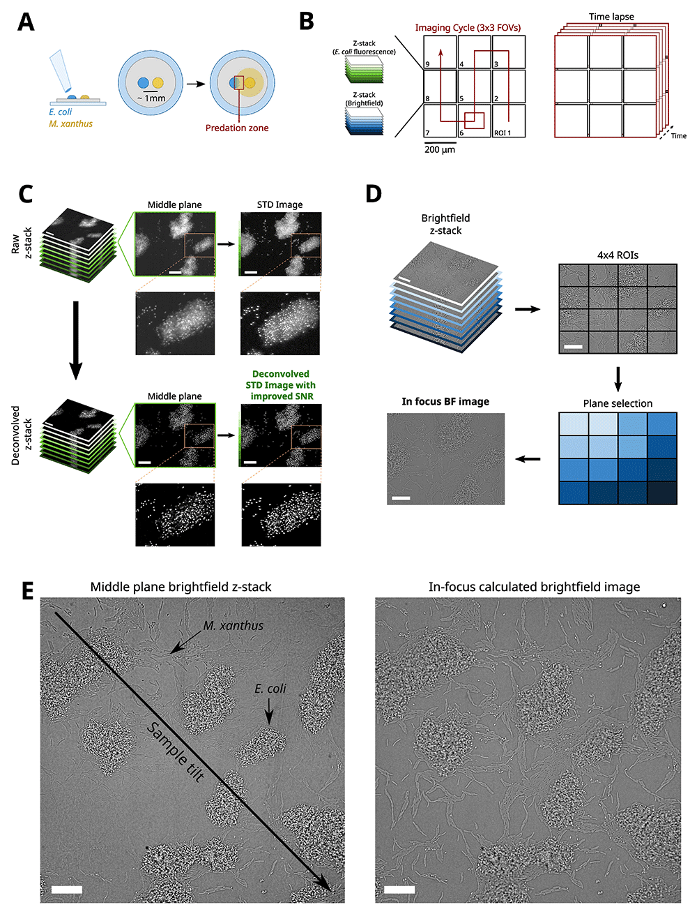
Figure 1.
A) Sample preparation of a predation assay. A colony of M. xanthus (yellow) is spotted at a millimeter distance from a colony of E. coli (blue) on a hard agar surface. This sample is then incubated for 48-72 hours before imaging the forefront of the predation zone (red boxed area). B) Mosaic imaging of the predation forefront. The region of interest (ROI) is imaged by dividing it into a 3-by-3 mosaic made up of 2048x2048 pixels Field Of Views (FOVs). For each FOV at least two z-stacks are acquired, one for the brightfield channel and one for the E. coli fluorescence channel. The acquisition of each mosaic FOV with its corresponding z-stacks acquired in a serpentine pattern makes up an imaging cycle. By repeating the acquisition of imaging cycles, a timelapse is constructed of the large ROI. C) Processing of E. coli fluorescence z-stacks to 2D images. The E. coli fluorescence z-stack is deconvolved and a 2D standard deviation image is calculated from the deconvolved z-stack to enhance the signal to noise ratio. Scalebars = 20 μm. D) Processing of the brightfield z-stacks to 2D images. The brightfield z-stack is divided into 4x4 blocks, and for each block the in-focus plane is selected. A 2D in-focus brightfield image is reconstituted by retaining all selected planes. Scalebars = 20 μm. E) In-focus calculation of brightfield images as a solution to sample tilt. Scalebars = 20 μm.
Acquisition of imaging data at relevant spatial and temporal scales requires a tradeoff between imaging areas large enough to capture collective cell displacements over long distances, and high imaging rates enabling the reconstruction of single cell trajectories over extended acquisitions. The imaging area provided by large-sensor sCMOS cameras (2048x2048 pixels) combined with a high magnification objective allowing for single-cell imaging (e.g., 60x) does not provide a sufficiently large area (0.05 mm²) to visualize events at scales relevant to the community. For instance, the area explored by M. xanthus cells ahead of the large collective cell groups (swarms) is ~0.05mm², to track at the same time the movement of single cells and swarms requires considerably larger imaging areas. To increase the size of the region tracked, we constructed 3-by-3 mosaic images by acquiring and tiling neighboring fields-of-view (FOV). A serpentine pattern was used to minimize stage displacement between successive images (Figure 1B). An overlap of 200 pixels (17µm) was used to allow for efficient and robust reassembly of tiles into a single image of ~ 0.36 mm². For each tile, brightfield and multiple fluorescence channels were imaged to enable the semantic segmentation of multiple bacterial species, and the subcellular localization of protein complexes.
To account for possible tilt in the sample or for agar pad deformation, 3D stacks spanning 3–4µm in the axial direction were acquired (7–9 planes, interspaced by 500nm). This allowed us to capture bacterial cells in-focus over a large FOV. An imaging cycle, corresponding to one time point in the timelapse, was completed when all z-stacks for each of the nine FOVs were acquired in both brightfield and fluorescence channels. Live axial drift correction based on the reflection of an infrared laser beam (785 nm) was used to maintain the focus during the course of the experiment (>6h). By repeating the 3-by-3 mosaic imaging cycle, a time lapse of a ~0.36mm² area of the predation assay was acquired.
Robust and efficient reconstruction of single cell tracks requires a minimal overlap of cell masks between consecutive acquisitions. E. coli cells are mostly immobile and M. xanthus cells move on average at 2-4 μm/min (Shi & Zusman, 1993) have a typical length of ~4-5 μm (Patra et al., 2016). Thus, to ensure a ~50% area overlap between consecutive frames, the acquisition time for a full 3x3, 3D, two-color mosaic image needs to be ~35s or smaller. To achieve this imaging time, we developed a fully-automated imaging routine written in LabView which synchronizes all the required hardware components: lasers, camera, piezo-electric z-stage, translation stage, field-programmable gate array (FPGA), and an autofocus system (see Microscopy section in Methods) (Cardozo Gizzi et al., 2019).
Finally, newly acquired stacks are pre-processed to improve the signal to noise ratio, and project the 3D image stack into a single in-focus 2D image. For the fluorescence channel, 3D-stacks were first deconvolved (see Treatment of fast time lapse data in Methods) and a 2D image was then calculated by computing the standard deviation projection of the deconvolved stack (Figure 1C). For the brightfield channel, in-focus 2D images were reconstructed in three steps (Figure 1D). First, the brightfield 3D-stack was subdivided into 16 blocks of 512x512 pixels. For each image of the blocks, the modulation transfer function was calculated by computing the line spread function along the x and y directions. The images with the sharpest features were then selected from each block and recombined into a single 2048x2048 in-focus image (Figure 1E).
AI-based semantic cell segmentation
To segment cells semantically, we developed a deep learning approach. This approach was based on a convolutional neural network (CNN) with a U-net architecture provided by Matlab R2019 (Ronneberger et al., 2015). The inputs of the network were an in-focus 2D bright-field image containing both M. xanthus and E. coli cells and a 2D standard deviation fluorescence image of fluorescently-labeled E. coli. For the U-net training, an image database was created and contained representative data from different experimental conditions, including images with either low or high M. xanthus cell densities (such as in swarms), small E. coli colonies, and both bacterial species in close spatial proximity or intermixed (Figure 2A). In total, forty 260-by-260 pixels images, composed of one brightfield image and the associated fluorescence image of E. coli nucleoid (HU-mCherry), were manually annotated using five distinct classes: i) background, ii) M. xanthus body, iii) M. xanthus contour, iv) E. coli body, and v) E. coli contour (Figure 2B). The contour of cells in densely packed regions was allowed to overlap and was included as a distinct class as this forced the network to spatially separate single cell bodies. From each annotated 260-by-260 pixels image, several 128-by-128 pixels training images were sampled. The training dataset was further expanded by calculating the annotated 45°-rotated 182-by-182 pixels image and sampling several training images from these calculated images. This allowed us to omit the time-consuming and labor intensive process of manually annotating numerous experimental images. To increase the robustness of the semantic segmentation slightly out-of-focus images were included for each image in the training dataset (Shorten & Khoshgoftaar, 2019). Finally, a classical data augmentation step was performed, including for example left-right and up-down flipping of the training images. Note that automatic rotation was not allowed for data augmentation during training since it often created mis-labeling errors (contour vs. body) when working with densely packed cells images. Finally, each pair of raw/labeled images were randomly assigned to either a training set (70% of the data), a validation set (15%) or a testing set (15%). Training was performed using a U-net architecture composed of an encoder-decoder depth of 3, filter size of 5x5x2, and allowing image augmentation (random up-down, left-right flip).
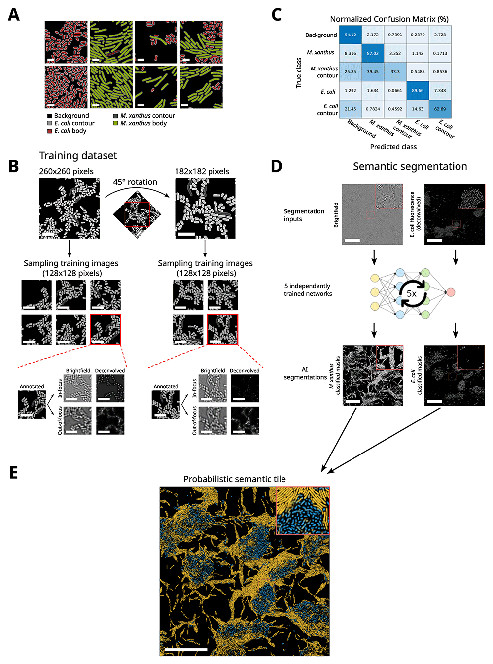
Figure 2. Semantic segmentation with MATLAB-based U-net algorithm.
A) Example of ground truth images. Images are annotated for the five classes: i) background, ii) E. coli body, iii) E. coli contour, iv) M. xanthus body, and v) M. xanthus contour. Scalebars = 2 μm. B) Example of an annotated image for the set-up of the training image database. From a 260x260 pixel image annotated for the ground truth, a number of training images (128x128 pixels) were sampled. For each sampled training image, several out-of-focus brightfield and fluorescence images were included as well. The 260x260 pixels image was then 45° rotated from which additional training images were sampled. Out-of-focus brightfield and fluorescence images were included again. Scalebars = 5 μm. C) Normalized Confusion Matrix for a trained U-net. From this matrix, the accuracy of pixel assignment to a given class predicted by the trained network is evaluated by comparing it to the ground truth. D) Semantic segmentation of experimental input images. The inputs for the U-net are brightfield and fluorescence images. Segmentation is performed by five independently trained networks that output an image containing the confidence value for each pixel for each class. Scalebars = 50 μm. E) A probabilistic semantic tile can be assembled visualizing the E. coli (blue) and M. xanthus (yellow) body classes. Scalebar = 50 μm.
The performance of the trained network, defined by the ability of a network to accurately classify a pixel, was evaluated by calculating the confusion matrix from the testing set (Figure 2C). The confusion matrix represents how well the network predicts the class of a given pixel using the ground truths of the testing set. The diagonal of the confusion matrix indicates how often the network properly predicts a class: for instance, 87% of the pixels annotated as M. xanthus cell body in the ground truth are predicted as M. xanthus cell body by the network. The non-diagonal terms indicate errors: for example, 1.142% of the M. xanthus cell body pixels are improperly assigned to E. coli cell body. Using this analysis, we observe that the trained network is able to efficiently differentiate M. xanthus from E. coli cells with >87% accuracy. The assignment of the M. xanthus and E. coli contour classes were often intermixed with the respective cell body class or the background. However, this did not pose a problem per se, as the classes for cell contour were only used to properly separate cell body masks in regions where cells were densely packed, and these improper pixel assignments are filtered out by filtering steps (see below).
Robust construction of single-cell trajectories from masks segmented at different time points could be compromised when cell masks in close physical proximity are not properly separated and merge into one large mask. To avoid this bias, we adopted a strategy in which five networks were independently trained (Figure 2D). Each network used a refocused 2D brightfield image and its corresponding 2D deconvolved fluorescence image as inputs and outputs the corresponding segmented image. Therefore, from the five networks, five slightly different segmentations are obtained, respectively for E. coli and M. xanthus cells. These images are combined into a probabilistic image with a confidence value ranging between 0 and 5 for the assignment of each pixel to either the class of E. coli or the class of M. xanthus, with 0 being the case where none of the five networks assigned the pixel to a given class and 5 being the case where all five networks assigned the pixel to a given class (Figure 2E). This strategy allowed us to perform a stringent segmentation of each single cell and to converge to an accurate result for which limited post-processing of the segmented masks was required for further analysis.
Reconstruction and registration of large-scale tiled images
Next, we developed a method to assemble the 3-by-3 mosaics, acquired every 35s into single images. For this, we used an iterative image cross-correlation algorithm that determines the overlap between any two neighboring images with pixel precision. To ensure smooth transitions between tiles in the final image, we combined tiles using an alpha blending method with a decreasing transparency gradient (Figure 3A). A typical acquisition that captures M. xanthus predation requires the imaging of the same region for extended time periods (~6h), during which the microscope stage drifts laterally mainly due to temperature variations. To account for lateral drift, we performed image registration for all time-points by cross-correlating assembled images of the E. coli segmented image with the reference image from the first time-point (Figure 3A).
Finally, probabilistic M. xanthus masks were converted to binary masks by applying several filtering steps (Figure 3B). These steps were included to resolve occasional merged masks and ensure that only true single-cell masks were included for the single-cell tracking of M. xanthus cells. First, we filtered pixels with high confidence values. For each mask, pixels in the perimeter with lower confidence values are retained only when the mask area does not increase more than 5% to avoid fusing neighboring cell masks. The output of this pixel selection procedure is a binary image with 4-connected M. xanthus cell masks. Second, M. xanthus masks with areas lower than 100 pixels were rejected to reinforce semantic segmentations, as typical M. xanthus cells contained several hundred pixels. An additional filtering, based on branchpoint detection and tortuosity, was applied to reject fused cell masks which could not be detected in the pixel selection step (Figure 3B). As M. xanthus are rod-shaped cells, their backbone is a line without any branchpoints. Pole-to-body mask fusions can thus be detected and rejected by calculating the backbone of all masks and identifying branch points (Figure 3B, green boxed area). Furthermore, pole-to-pole mask fusions for which no branchpoint could be calculated were detected by calculating the tortuosity, which is a measure of curvature, of the mask defined as the ratio between the length of the backbone and the distance between the endpoints of the backbone. The mask was rejected when the tortuosity exceeded the threshold of two (Figure 3B, red boxed area). The masks retained after these post-processing steps were used to construct the final assembled images and to reconstruct single-cell trajectories, as described in the next section (Figure 3C).
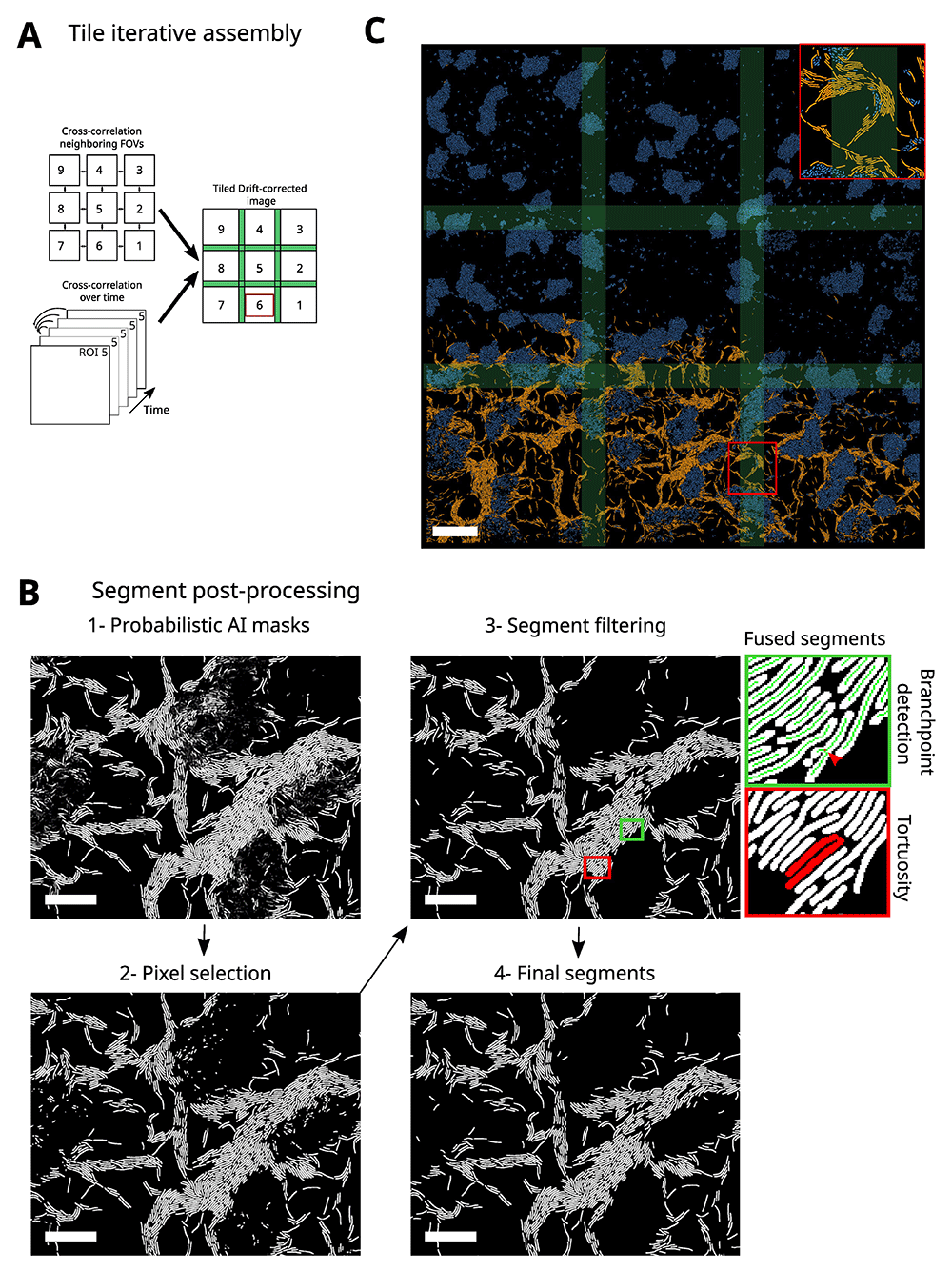
Figure 3. Image post-processing.
A) Image post-processing to reassemble a large ROI and to correct drift. By calculating the cross correlation of the overlap region (green area in the final processed image) between neighboring FOVs, their corresponding pixel-precise positioning in the mosaic can be determined. After the tiling of the mosaic, a drift correction is applied based on the cross-correlation between the middle FOV at time t with the middle reference FOV reference at time t=1. B) Post-processing of the segments to reject all improper masks. Raw probabilistic M. xanthus AI masks are first converted to a binary image by selecting pixels based on their confidence values (1), masks are then filtered for size and finally fused masks are rejected based on backbone branch points (green boxed area) and tortuosity (red boxed area) (2). Scalebars= 20 μm. C) Final assembled, drift-corrected, and post-processed semantic masks of M. xanthus (yellow) and E. coli (blue). Scalebar = 50 μm.
Single-cell tracking
The construction of single-cell M. xanthus trajectories requires robust algorithms that link together masks from the same cell acquired at different time points. A method that relies exclusively on the maximization of overlap between cell masks at consecutive time points works well for isolated cells, but not in more challenging conditions where cells are densely packed in space (e.g., swarms). To deal with cells in these dense regions, we developed an analysis method that uses, in addition to the overlap of masks between consecutive time points, multiple morphological mask parameters and a ranking approach.
Specifically, this approach consists of three distinct stages: i) pairwise tracking, ii) filtering of pairwise tracks, and iii) track reconstruction. In the first stage, we connected pairs of masks detected in consecutive time frames by constructing, for each mask at time t, the list of candidate masks at time t+1. Candidates were selected by finding the masks at time t+1 that partially overlapped with the dilated bounding box of the cell of interest at time t. Three scenarios were frequent: (i) no candidate was found, making it impossible to make a pairwise connection between the cell of interest and its candidate; (ii) a unique suitable candidate was found, a typical scenario for isolated cells, allowing a straightforward pairwise connection between the masks at times t and t+1; and (iii) multiple candidates were found, a typical case for groups of cells, making several pairwise connections possible. When multiple candidates were found, we calculated the cell length, the mask area and their overlap for the cell of interest and for the candidates. These parameters were used as inputs for Analytical Hierarchy Processing (AHP), a method that ranks all the possible pairwise associations from most to least likely (Saaty, 1986) and thus, allowed us to select the most likely pairwise association (Figure 4A). The process of candidate selection and pairwise association was iteratively repeated for all cell masks at time t.
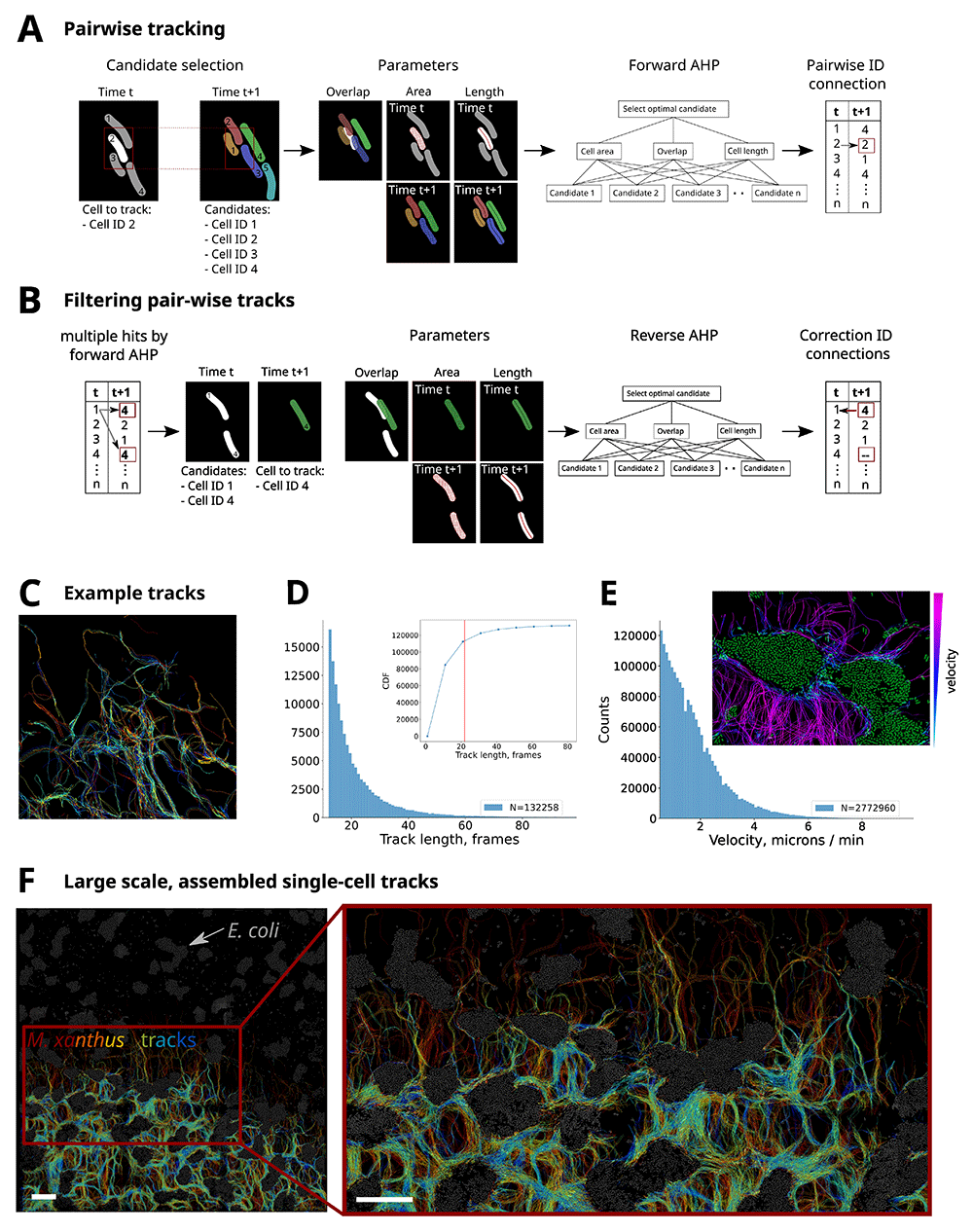
Figure 4. Schematic of single-cell tracking method.
A) Pairwise tracking to connect all masks at time t to their corresponding masks at time t+1. For each mask at a given time point (time t), candidate masks for connection are selected in the consecutive time point (time t+1) based on the bounding box of the mask (t). For the mask (t) and candidates (t+1), three parameters are calculated: i) the cell length based on its backbone, ii) the cell area and the overlap between the mask (t) and iii) the mask of the candidate (t+1). These parameters are the input for the Analytical Hierarchy Processing (AHP) which ranks the candidates from most suitable to least suitable for connection. This process is repeated for all masks (t) and results in a list of pairwise connections. B) Filtering and correction of multiple assignments in pairwise connection lists. To account for multiple assignments of a candidate, a reverse AHP step is included in which the most suitable mask (t) is selected for the candidate (t+1). The list of pairwise connections is then corrected, for masks (t) that were not selected in the reverse AHP, the trajectory is stopped. C) Selection of single M. xanthus tracks color-coded by track identity in a region of interest of 115µm. Only a small number of tracks are represented (N = 383) for clarity. D) Histogram of track lengths for the full dataset. Inset displays the cumulative distribution function. Red line indicates the mean track length. N = 132258 indicates the number of tracks. E) Histogram of track instant velocities (N = 2772960 tracks). Inset: region of the 3-by-3 mosaic where E. coli masks are shown in green and M. xanthus tracks are displayed according to their velocity (see colormap on the right). F) Example of reconstructed tracks in a 3-by-3 mosaic for a full experiment (700 time points). E. coli cells are shown in gray. M. xanthus tracks are color-coded by time. Scalebars = 50 μm.
For cells in densely packed regions, multiple assignments of the same candidate at time t+1 could occur, indicating that the same candidate at time t+1 was selected for pairwise association with two or more cells of interest at time t (Figure 4B). To resolve such conflicts, we implemented a filtering step in which these multiple assignments were detected and retained. Then, to connect the correct pair of masks, a reverse strategy was used in which the mask at time t+1 became the cell to track and the masks at time t became the candidates. Similarly, as before, the parameters for cell length, mask area and overlap were used as inputs for the AHP, allowing us to rank the pairwise associations and select the most likely connection. This filtering step finally results in a list of unique pairwise connections, essential for more robust track reconstruction.
After reconstructing and filtering the pairwise associations for all sets of consecutive images, full-length tracks were assembled by iteratively connecting cell IDs from pairwise tracks (Figure 4C). We note that while this methodology considerably improves the robustness of track reconstruction, it still has limitations. A specific limitation is its ability to track M. xanthus cells within regions containing multiple cell layers, for instance within E. coli islands or in extremely large swarms. In these cases, our algorithm selects and analyzes the focal plane where most cells are in-focus, thus missing in the process out-of-focus cells whose tracks cannot be properly completed. We envision that development of 3D AI segmentation methods will be necessary to bypass this limitation.
Time-lapse experiments in 3x3 mosaics covering ~0.36 mm2 at 35s time resolution were used to obtain full-length single cell trajectories. An example of the final tracks can be visualized in the Extended Data 1. These trajectories can be used to characterize the tracking process, for example through the track length distribution (Figure 4D). On average, cells were tracked for ~22 frames = 768s. The ability of our algorithm to reconstruct longer tracks was limited by cells leaving the imaging area, and by the tracking of out-of-focus cells (see above), or within extremely high-density areas where our reconnection approaches were unable to converge to a unique solution or when masks were filtered out due to segmentation errors (see Figure 3B). Despite these limitations, the high-throughput of our method enabled the reconstruction of thousands of long tracks: >19,000 tracks more than ~770s-long.
In addition to track lengths, single-cell trajectories can be used to calculate dynamic properties, such as the distribution of instant speeds (Figure 4E). The measured speeds are consistent with speeds previously reported in the literature (2-4 μm/min) (Shi & Zusman, 1993). We note that an interesting feature of our approach is that track properties (such as speed) can be used to detect spatial changes in single cell dynamic behaviors. For instance, by embedding speed into cell masks we observe that M. xanthus cells have the tendency to slow down when they reach E. coli islands (Figure 4E, inset).
Finally, representation and analysis of thousands of tracks over mm-scales permits the monitoring of large-scale single-cell dynamics over biologically-relevant timescales (Figure 4F), such as migration of M. xanthus between E. coli islands during predation.
Discussion
In this article, we propose an imaging, cell segmentation and tracking framework for the study of predation of M. xanthus on E. coli. Our high-throughput, high resolution microscopy method allows the acquisition of large imaging areas in a timelapse manner by employing a mosaic imaging scheme. We propose a deep learning-based semantic segmentation approach for the reconstruction of single-cell M. xanthus and E. coli masks. And finally, we present a method that enables the tracking of motile M. xanthus cells.
The workflow proposed here allowed us to overcome several challenges for capturing single-cell dynamics of complex multicellular systems. First, mosaic imaging allows the visualization of extensive areas without sacrificing resolution and thus, thousands of single-cells can be tracked together with their position within the community to provide spatial context. Mosaic approaches are widely used for the imaging of fixed biological specimens, such as tissue slices (Chow et al., 2006; Price et al., 2006) and are often incorporated in commercial microscopes. However, we found that their adaptation to dynamic imaging requires certain tradeoffs, particularly constraining when multi-color, multimodal, and multi-plane acquisitions are required. Specifically, the maximum imaging area scales linearly with the acquisition time per mosaic (~35s, in our case defined by the time needed for a cell to travel half its length). This relation implies that increases in the imaging area can be achieved by shortening the time required for the acquisition of a single tile, or by slowing the system dynamics (i.e., cell speed). The robotic microscope we implemented enabled the acquisition of 3x3 tiles at frame rates able to capture the relevant biological timescales in our predation assay. We note that further reduction of the acquisition time could be achieved by resorting to multi-focus systems using multiple cameras to acquire several planes at once (Chao et al., 2017), or by removing the need to acquire multi-modal, multi-focus datasets. Alternatively, remote refocusing techniques (Botcherby et al., 2008) which are becoming increasingly popular for rapid, 4D optical imaging (https://andrewgyork.github.io/remote_refocus/appendix.html) would considerably reduce the acquisition time of single volumes. We envision that the use of oblique-plane microscopes could also contribute in future to the high-resolution acquisition of large complex samples, such as biofilms, with reduced acquisition times (Sapoznik et al., 2020).
An important challenge arising from the acquisition method we developed is the handling, analysis and storage of large numbers of images (~1000 3D, multi-channel volumes per experiment). We solved this challenge by resorting to automatic, robust image analysis tools that required minimal user input. For this, we used a deep learning method based on the U-net architecture, similar to our recent development (Panigrahi et al., 2021), to segment and identify multiple species in millimeter-sized 2D images. The field of image analysis using deep-learning is moving fast (Greener et al., 2021; Hallou et al., 2021) and more robust, and flexible possibilities are likely to emerge in future. For instance, the use of 3D AI-based segmentation will likely be capable of semantically segmenting bacterial cells within multi-layered samples, such as biofilms (Weigert et al., 2020; Zhang et al., 2020), thus enabling the tracking of cells in multi-layers.
Finally, we implemented an algorithm to reconstruct single-cell trajectories of motile M. xanthus cells from single cell masks. By using a ranking approach for complex decision making (Saaty, 1986), we were able to improve the tracking of cells in different environments, including cells in isolation, in small groups, and in larger swarms. Other bacterial cell segmentation algorithms were developed in the past for the tracking of bacterial cells at low densities, in mother-machines, or for lineage tracing (reviewed in (Jeckel & Drescher, 2021)). However, these methods are either ill-adapted for robust, automatic analysis required of high-throughput tracking datasets, for semantic detection of different species, or for single-cell tracking within complex communities displaying high cell densities. More recently, a new approach using deep-learning to retrieve single-cell tracks for lineage tracking was developed (O’Connor et al., 2022). However, this development does not perform semantic segmentation, and it is unclear how it will perform on bacteria with curved shapes (such as M. xanthus), or in samples with large number of cells, high cell densities, or with multi-layers. A main challenge ahead will be to improve the efficiency of detection, 3D segmentation and tracking of single cells within densely packed multilayers, such as those encountered in biofilms. Taken together, this workflow opens the door for the quantitative study of bacterial predation of M. xanthus on E. coli. In addition, we predict that this workflow should be easily used to study other complex and multispecies systems.
Conclusion
In this paper, we presented several methods for the acquisition and analysis of the dynamics of single bacterial cells within complex micro-environments. For this, we developed a hardware-accelerated, automated microscope to robustly image large areas of the sample, over long periods of time, and with high temporal resolution. Next, we applied a UNET-based, deep-learning approach to semantically segment single bacterial cells within densely-packed cell groups. Third, we designed a cell tracking algorithm to track single motile cells. Finally, we applied these technologies to the predation of E. coli by M. xanthus and extracted dynamic track parameters from thousands of single-cell tracks with spatial resolution. In this paper, we presented several methods for the acquisition and analysis of the dynamics of single bacterial cells within complex micro-environments. For this, we developed a hardware-accelerated, automated microscope to robustly image large areas of the sample, over long periods of time, and with high temporal resolution. Next, we applied a UNET-based, deep-learning approach to semantically segment single bacterial cells within densely-packed cell groups (Nollmann, 2022c). Third, we designed a cell tracking algorithm to track single motile cells. Finally, we applied these technologies to the predation of E. coli by M. xanthus, and extracted dynamic track parameters from thousands of single-cell tracks with spatial resolution.