Plain language summary
The dataset here presented is very useful for oceanographers, marine biologists, and chemists in an idealized scenario with no river runoff (Amazon River and Pará River) in the western tropical North Atlantic (WTNA). You can study the ocean properties (for example, temperature, salinity, and currents), the influence of the chemical components (for example, nutrients and CO2 fluxes), and the biological relations of different organisms and their distribution at the region. With these simulation results, you can compare the observed data you are working on with our numerical ocean model outputs, estimating the influence of the Amazon and Pará Rivers in this region. These data are stored in the following formats: ROMS model NetCDF, Matlab, and NetCDF standard. In the case of Matlab and NetCDF standard, no pre-processing is required. Moreover, the dataset is available in the open repository of Science Data Bank (doi: 10.57760/sciencedb.02145), and to access click here.
Introduction
The western tropical North Atlantic (WTNA) is characterized as an extremely complex region with the influence of different physical forcings, such as strong western boundary currents (e.g. North Brazil Undercurrent and North Brazil Current) in connection with zonal equatorial currents (e.g South Equatorial Undercurrent, Equatorial Undercurrent, and North Equatorial Countercurrent) as part of the equatorial current system1; important atmospheric drivers (e.g trade winds and the Intertropical Convergence Zone)2; and mesoscale activity (e.g NBC rings)3,4. Besides, the region also presents an important pathway of interhemispheric transport of mass, heat, and salt as part of the Atlantic Meridional Overturning Circulation5,6.
A singular aspect of this region is the presence of the Amazon River runoff, the world’s largest river discharge accounting for 18% of the continental water flow to the oceans and approximately 32% of the freshwater input to the Atlantic ocean, with an average of 222,800 m3 s−17,8. The discharge volume reaches up to two-fold the net atmospheric freshwater flux (evaporation-precipitation) over the WTNA9. Furthermore, the Amazon River forms a plume over the region, which extends over a thousand of kilometers, flowing northwestward and reaching the Caribbean Sea and also retroflecting eastward through the North Equatorial Countercurrent and reaching latitudes of 30°W10,11. Therefore, the region is marked by an intense land-ocean synergy, with several processes in play, such as mixed layer depth changes and formation of barrier layers, leading variations of the ocean surface heat balance12,13; high terrestrial sediments and dissolved organic matter transport11; and complex and important biogeochemical interactions, from nutrient and carbon fluxes14,15 to changes on biological community structures16.
The present work brings a dataset originated from simulations using the regional oceanic modeling system (ROMS) model in an idealized scenario of no river runoff of the Amazon River and the Pará River in the WTNA. The main goal for the creation of the here presented dataset is to enable and encourage the development of more researches in the region to advance in bridging the knowledge gaps of a such complex area. In the following Sections, we present the methods, which introduces the study area and explains the model configuration, the initial and boundary parameters; the dataset, with the directory structure of the dataset, the generated files, and details of the coordinates and variables of each of the generated files; and lastly, the data availability.
Methods
This study was conducted through ideal simulations with the ROMS numerical model, using the ROMS-AGRIF version (regional ocean modeling system - adaptive grid refinement)17–20, which has been successfully tested in the WTNA, specifically off the North and Northeastern Brazilian coast12,21–31. The geographic localization of this dataset is 60.5°-24°W/5°S-16°N, which is illustrated in Figure 1 with the monthly sea surface temperature (SST) horizontal distribution in the period maximum Pará River runoff (March-April) and maximum Amazon River runoff (May-June)7. In these four months, the minimum SST found in the area corresponding to this dataset is 35 psu (practical salinity unit), with values reaching 32 psu over the river plume and 27 psu off the Amazon River mouth29.
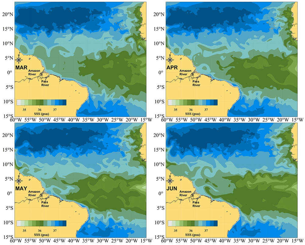
Figure 1. Geographic location of the dataset.
Sea Surface Salinity field in the periods of maximum Pará River runoff (March–April, upper panels) and maximum Amazon River runoff (May–June, lower panels).
For our simulation, all initial and boundary parameters have been spatially discretized at a horizontal resolution of 0.25° with non-isotropic grid from Earth Topography v2 (ETOPO2) bathymetry32 and vertically using the sigma coordinate system (32 vertical levels). In the configuration file (ROMSTOOLS; romstools_param.m), ROMSTOOLS is a set of Octave compatible Matlab functions used to perform pre-processing of ROMS model input data, we used theta_s = 6 and theta_b = 0 (These two parameters indicate to the ROMS model how it has to consider the distribution of vertical levels near the surface and the bottom, both must take values between zero and seven, the higher the values of these, the more vertical levels will be concentrated near the surface and the bottom)19,33, obtaining 12 and 20 levels in the first 100m and 500m depth, respectively. Other parameters used in the grid discretization are: hc = 5.0, hmin = 150, hmax_coast = 500, hmax = 5000, rtarget = 0.25 (slope), and Roa = 85e3.
Since tidal influence is important for the seawater mixing process in the surface layers, tides have been taken into account in our simulation and data were obtained from OSU TPXO7 Tide model34,35. The North, South, East and West lateral boundaries were considered open and the sea surface salinity (SSS) and sea surface temperature (SST) values for initial and boundary conditions were restricted to monthly mean values obtained from the World Ocean Atlas 2009 (WOA2009 dataset)36,37. For the surface forcing, it was used monthly climatology of the Comprehensive Ocean-Atmosphere Data Set (COADS05 dataset)38. This dataset is the last year of the numerical output (roms_his.nc and roms_avg.nc) obtained by a ROMS-model simulation of 11 years, and it was called the No-River Runoff experiment (NRF) in 27,29.
Dataset
The idealized hydrodynamical numerical model database with no-river runoff in the Northern and Northeastern Brazilian coast (IHMD-NRF) is the result of a research carried out by 29. As shown in Table 1, the dataset includes three pairs of files: (i) ROMS-files as two files in ROMS NetCDF format, containing the monthly and weekly numerical output (raw data); (ii) MATLAB-files as two files processed and converted in Matlab; and (iii) NetCDF-files as two more files also processed and converted in NetCDF standard format with mNC tool39, the file pairs in (ii) and (iii) are identical to (i), but have been converted to Matlab formats (they can be read in Octave, R and Python) and the NetCDF standard. For each file, some metadata were added using freeware tools called Climate Data Operator (CDO)40 and NetCDF Operators (NCO)41. All files are organized in the directory structure shown in Figure 2.
Table 1. Files that integrate this dataset and its main characteristics.
| Filename | Description | Format | Processing level | Size |
|---|
| roms_his_Y11.nc | ROMSfile of monthly climatology of the ROMS simulation | ROMS
NetCDF | Raw data | 351 Mb |
| roms_avg_Y11.nc | ROMSfile of weekly climatology of the ROMS simulation | ROMS
NetCDF | Raw data | 1.4 Gb |
| SR_MonthlyClim.mat | MATLABfile of monthly climatology of the ROMS simulation | Matlab | Processed data | 694 Mb |
| SR_WeeklyClim.mat | MATLABfile of weekly climatology of the ROMS simulation | Matlab | Processed data | 2.7 Gb |
| SR_MonthlyClim.nc | NetCDFfile of monthly climatology of the ROMS simulation | NetCDF
standard | Processed data | 1.1 Gb |
| SR_WeeklyClim.nc | NetCDFfile of weekly climatology of the ROMS simulation | NetCDF
standard | Processed data | 4.5 Gb |
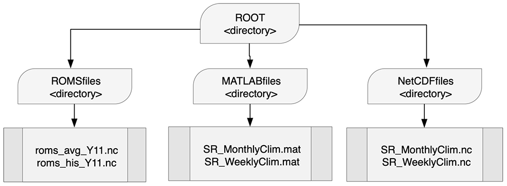
Figure 2. Distribution of files by directory according to their format.
The ROMSfiles directory stores the ROMS model numerical output files for monthly and weekly data for the 11th year.
The outputs’ dimensions, their description and dimension size are listed in Table 2. The parameter time does not need any conversion when working with MATLAB, the function datestr provides the date. The monthly output is dated on the first day of each month, while the weekly output is on the 4th, 12th, 19th and 27th of each month. The year of this date is relative to the simulation year, so it will always be 0011 (11th year). Table 2 shows the time parameter twice, once at monthly and once at weekly frequency, corresponding to each of the ROMS-files outputs. In the monthly output file (rooms_his_Y11.nc), there are 13 values because January - year 0012 is also included.
Table 2. ROMS-files dimensions (coordinate system parameters).
| Dimensions | Description | Variable dimension |
|---|
| xi_rho | Longitude dimension for scalar variables | 185 |
| eta_rho | Latitude dimension for scalar variables | 161 |
| s_rho | Vertical levels for all variables | 32 |
| time | Time values, weekly climatology | 48 |
| time | Time values, monthly climatology | 13 |
| xi_u | Longitude dimension for vector variable | 184 |
| eta_v | Latitude dimension for vector variable | 160 |
The current velocity component (vector) grids have 184 × 160 nodes, while the scalar parameter grids have 185 × 161 nodes. Still for the ROMSfiles, Table 3 shows all the variables, which are related to the oceanographic and surface physical parameters. Other complementary descriptions of the ROMS model output files, i.e ROMS-files, can be found in 42, 43. All the ROMS model output files that are in the directory can be visualized with the tools that are in the directory called Roms_tools/Visualization_tools/. The folder is a component of ROMSTOOLS, the main script is roms_gui and it is a graphical user interface (GUI)19,33. This GUI is developed in MATLAB GUIDE (Octave-compatible), so it allows you to reuse other functions to retrieve parameters at a given level or depth, or even at a specific coordinate or date, e.g.: get_var.m.
Table 3. ROMSfiles variables (oceanographic and surface parameters) contained in the ROMSfiles directory.
| Variables | Description | Unit |
|---|
| lon_rho | Horizontal nodes longitude | Degrees east |
| lat_rho | lat_rho Horizontal nodes latitude | Degrees north |
| lon_u | Horizontal nodes longitude | Degrees east |
| lat_u | Horizontal nodes latitude | Degrees north |
| lon_v | Horizontal nodes longitude | Degrees east |
| lat_v | Horizontal nodes latitude | Degrees north |
| h | Bathymetry | m |
| temp | Potential temperature | °C |
| salt | Salinity | PSU |
| u | u-momentum component | m s−1 |
| v | v-momentum component | m s−1 |
| w | Vertical momentum component | m s−1 |
| zeta | Sea Surface Height | m |
| ubar | Vertically integrated u-momentum component | m s−1 |
| vbar | Vertically integrated v-momentum component | m s−1 |
| f | Coriolis parameter | s−1 |
| bostr | Kinematic bottom stress | N s−1 |
| wstr | Kinematic wind stress | N s−1 |
| sustr | Kinematic u wind stress component | N s−1 |
| svstr | Kinematic v wind stress component | N s−1 |
| diff3d | Horizontal diffusivity coefficient | - |
| hbl | Depth of planetary boundary layer | m |
| hbbl | Depth of bottom boundary layer | m |
| shflux | Surface net heat flux | W m−2 |
| swflux | Surface freshwater flux (E-P) | cm day−1 |
| swrad | Short-wave surface radiation | W m−2 |
| swrad | Short-wave surface radiation | W m−2 |
| mask_rho | Land mask (0 to land, 1 to ocean) | - |
| mask_u | Land mask (0 to land, 1 to ocean) | - |
| mask_v | Land mask (0 to land, 1 to ocean) | - |
The two pairs of files, i.e MATLAB-files and NetCDF-files, contain oceanographic parameters such as salinity, temperature, sea currents, sea surface height (SSH), seawater density, and vorticity (Table 4 and Table 5). Here we present the descriptions of the oceanographic parameters in standard MATLAB and NetCDF formats (stored in the MATLABfiles and NetCDFfiles directories, respectively), all these files can be read in ncview, Panoply, CDO, NCO and other freewares like Octave, R and Python. In both cases, the time parameter has dimension size of 12 for each month of the 11th year of the monthly simulation and it also presents dimension size of 48 for the weekly simulation, with output on the same dates as the equivalent files in NetCDF ROMS format (ROMS-files). In these four pairs of files, the vector and scalar data grids are referenced with the same coordinate system.
Table 4. MATLAB-files variables (oceanographic parameters) contained in the MATLABfiles directory.
| Variables | Description | Unit |
|---|
| Lons | Horizontal nodes longitude | Degrees east |
| Lats | Horizontal nodes latitude | Degrees north |
| Time | Time | Months |
| DEPTHS | Depths | m |
| bathymetry | Bathymetry | m |
| temp | Potential temperature | °C |
| salt | Salinity | PSU |
| ssh | Sea Surface Height | m |
| u | u-momentum component | m s−1 |
| v | v-momentum component | m s−1 |
| rho | Seawater density | Kg m−3 |
| currspd | Current speed | m s−1 |
| vort | Vorticity | s−1 |
Table 5. NetCDF-files variables (oceanographic parameters) contained in the NetCDFfiles directory.
| Variables | Description | Unit |
|---|
| lon | Horizontal nodes longitude | Degrees east |
| lat | Horizontal nodes latitude | Degrees north |
| time | Time | Months |
| depth | Depths | m |
| h | Bathymetry | m |
| temp | Potential temperature | °C |
| salt | Salinity | PSU |
| ssh | Sea Surface Height | m |
| ucurr | u-momentum component | m s−1 |
| vcurr | v-momentum component | m s−1 |
| swd | Seawater density | Kg m−3 |
| cspd | Current speed | m s−1 |
| vort | Vorticity | s−1 |
The standard NetCDF files, i.e NetCDF-files, are self-describing as it is possible to explore a very detailed description of the metadata with the ncdump command in terminal44. You can also preview the data using the ncview command in terminal45, GrADS46 and Panoply data viewer47, the latter depending on the Java Runtime Environment.
Data availability
Underlying data
Science Data Bank: Idealized hydrodynamical numerical model database with no river runoff in the northeastern and northern regions of Brazil (IHMD-NRF) https://doi.org/10.57760/sciencedb.02145
This project contains the following underlying data:
- roms_his_Y11.nc (Monthly climatology raw data)
- roms_avg_Y11.nc (Weekly climatology raw data)
Extended data
Science Data Bank: Idealized hydrodynamical numerical model database with no river runoff in the northeastern and northern regions of Brazil (IHMD-NRF) https://doi.org/10.57760/sciencedb.02145
This project contains the following underlying data:
- SR_MonthlyClim.mat (Monthly climatology of ROMS simulation in MATLAB format)
- SR_WeeklyClim.mat (Weekly climatology of ROMS simulation in MATLAB format)
- SR_MonthlyClim.nc (Monthly climatology of ROMS simulation in NetCD format)
- SR_WeeklyClim.nc (Weekly climatology of ROMS simulation in NetCD format)
Data are available under the terms of the Creative Commons Attribution 4.0 International license (CC-BY 4.0).
Acknowledgments
The authors thank the Tropical and South Atlantic climate-based marine ecosystem predictions for sustainable management (TRIATLAS project), the Brazilian Research Network on Global Climate Change (Rede CLIMA) and the International Joint Laboratory TAPIOCA (IRD-UFPE-UFRPE) for the support received.
Faculty Opinions recommendedReferences
- 1.
Goes M, Molinari R, da Silveira I, et al.:
Retroflections of the north brazil current during february 2002.
Deep Sea Res 1 Oceanogr Res Pap.
2005; 52(4): 647–667. Publisher Full Text
- 2.
Stramma L, Rhein M, Brandt P, et al.:
Upper ocean circulation in the western tropical atlantic in boreal fall 2000.
Deep Sea Res 1 Oceanogr Res Pap.
2005; 52(2): 221–240. Publisher Full Text
- 3.
Johns WE, Lee TN, Schott FA, et al.:
The north brazil current retroflection: Seasonal structure and eddy variability.
J Geophys Res Oceans.
1990; 95(C12): 22103–22120. Publisher Full Text
- 4.
Fratantoni DM, Richardson PL:
The evolution and demise of north brazil current rings.
J Phys Oceanogr.
2006; 36(7): 1241–1264. Publisher Full Text
- 5.
Schmitz WJ Jr, McCartney MS:
On the north atlantic circulation.
Rev Geophys.
1993; 31(1): 29–49. Publisher Full Text
- 6.
Lumpkin R, Speer K:
Global ocean meridional overturning.
J Phys Oceanogr.
2007; 37(10): 2550–2562. Publisher Full Text
- 7.
Dai A, Trenberth KE:
Estimates of freshwater discharge from continents: Latitudinal and seasonal variations.
J Hydrometeorol.
2002; 3(6): 660–687. Publisher Full Text
- 8.
Barthem RB, Charvet-Almeida P, Montag LFA, et al.:
Amazon basin: Global international waters assessment (giwa) regional assessment 40b.
Technical report, United Nations Environment Programme (UNEP),
2004.
- 9.
Ferry N, Reverdin G:
Sea surface salinity interannual variability in the western tropical atlantic: An ocean general circulation model study.
J Geophys Res Oceans.
2004; 109(C5). Publisher Full Text
- 10.
Lentz SJ:
The amazon river plume during amasseds: subtidal current variability and the importance of wind forcing.
J Geophys Res Oceans.
1995; 100(C2): 2377–2390. Publisher Full Text
- 11.
Coles VJ, Brooks MT, Hopkins J, et al.:
The pathways and properties of the amazon river plume in the tropical north atlantic ocean.
J Geophys Res Oceans.
2013; 118(12): 6894–6913. Publisher Full Text
- 12.
Silva AC, Araujo M, Medeiros C, et al.:
Seasonal changes in the mixed and barrier layers in the western equatorial atlantic.
Braz J Oceanogr.
2005; 53(3–4): 83–98. Publisher Full Text
- 13.
Grodsky SA, Reverdin G, Carton JA, et al.:
Year-to-year salinity changes in the amazon plume: Contrasting 2011 and 2012 aquarius/sacd and smos satellite data.
Remote Sensing of Environment.
2014; 140: 14–22. Publisher Full Text
- 14.
Chen CTA, Huang TH, Fu YH, et al.:
Strong sources of co2 in upper estuaries become sinks of co2 in large river plumes.
Curr Opin Environ Sustain.
2012; 4(2): 179–185. Publisher Full Text
- 15.
Araujo M, Noriega C, Lefèvre N:
Nutrients and carbon fluxes in the estuaries of major rivers flowing into the tropical atlantic.
Front Mar Sci.
2014; 1: 10. Publisher Full Text
- 16.
Stukel MR, Coles VJ, Brooks MT, et al.:
Top-down, bottom-up and physical controls on diatom-diazotroph assemblage growth in the amazon river plume.
Biogeosciences.
2014; 11(12): 3259–3278. Publisher Full Text
- 17.
Shchepetkin AF, McWilliams JC:
A method for computing horizontal pressure-gradient force in an oceanic model with a nonaligned vertical coordinate.
J Geophys Res Oceans.
2003; 108(C3). Publisher Full Text
- 18.
Shchepetkin AF, McWilliams JC:
The regional oceanic modeling system (roms): a split-explicit, free-surface, topography-following-coordinate oceanic model.
Ocean Model (Oxf).
2005; 9(4): 347–404. Publisher Full Text
- 19.
Penven P, Debreu L, Marchesiello P, et al.:
Evaluation and application of the roms 1-way embedding procedure to the central california upwelling system.
Ocean Model (Oxf).
2006; 12(1–2): 157–187. Publisher Full Text
- 20.
Debreu L, Mazauric C:
Adaptive grid refinement (agrif) in fortran 90: Users guide version 1.3. 2006. Reference Source
- 21.
Silva AC, Bourles B, Araujo M:
Circulation of the thermocline salinity maximum waters off the northern brazil as inferred from in situ measurements and numerical results.
Ann Geophys.
2009; 27(5): 1861–1873. Publisher Full Text
- 22.
Silva M, Araujo M, Servain J, et al.:
High-resolution regional ocean dynamics simulation in the southwestern tropical atlantic.
Ocean Model (Oxf).
2009; 30(4): 256–269. Publisher Full Text
- 23.
da Silva AC, Araujo M, Bourlès B:
Seasonal variability of the amazon river plume during revizee program.
Tropical Oceanography.
2010; 38(1): 76–87. Publisher Full Text
- 24.
Newinger C, Toumi R:
Potential impact of the colored amazon and orinoco plume on tropical cyclone intensity.
J Geophys Res Oceans.
2015; 120(2): 1296–1317. Publisher Full Text
- 25.
Tchamabi CC, Araujo M, Silva M, et al.:
A study of the brazilian fernando de noronha island and rocas atoll wakes in the tropical atlantic.
Ocean Model (Oxf).
2017; 111: 9–18. Publisher Full Text
- 26.
Tchamabi CC, Araujo M, Silva M, et al.:
Ichthyoplankton transport around the brazilian fernando de noronha archipelago and rocas atoll: Are there any connectivity patterns?
Indian J Mar Sci.
2018; 47(4): 812–818. Reference Source
- 27.
Varona HL:
Circulation, transport and dispersion of hydrocarbon plumes in the North Brazilian equatorial broadband.
Zenodo.
PhD thesis, Universidade Federal de Pernambuco, 2018. Publisher Full Text
- 28.
Varona HL, Silva MA, Veleda D, et al.:
Influence of underwater hydrodynamics on oil and gas blowouts off amazon river mouth.
Tropical Oceanography.
2018; 46(1). Publisher Full Text
- 29.
Varona HL, Veleda D, Silva M, et al.:
Amazon river plume influence on western tropical atlantic dynamic variability.
Dyn Atmos Oceans.
2019; 85: 1–15. Publisher Full Text
- 30.
de Santana CS, de Albuquerque Lira SM, Varona HL, et al.:
Amazon river plume influence on planktonic decapods in the tropical atlantic.
J Mar Syst.
2020; 212: 103428. Publisher Full Text
- 31.
Capuano TA, Araujo M, Silva M, et al.:
T-S and hydrodynamical structures within the deltaic regions and continental platforms adjacent to two northeastern Brazilian rivers.
Reg Stud Mar Sci.
2022; 51: 102219. Publisher Full Text
- 32.
Smith WHF, Sandwell DT:
Global sea floor topography from satellite altimetry and ship depth soundings.
Science.
1997; 277(5334): 1956–1962. Publisher Full Text
- 33.
Penven P, Cambon G, Tan TA, et al.:
Romstools user’s guide.
Rapport techn., IRD and LPO/UBO, Laboratoire de Physique des Oceans, Universite de Bretagne Occidentale/UFR Sciences.
2003.
- 34.
Egbert GD, Bennett AF, Foreman MGG:
Topex/poseidon tides estimated using a global inverse model.
J Geophys Res Oceans.
1994; 99(C12): 24821–24852. Publisher Full Text
- 35.
Egbert GD, Erofeeva SY:
Efficient Inverse Modeling of Barotropic Ocean Tides.
J Atmos Ocean Technol.
2002; 19(2): 183–204. Publisher Full Text
- 36.
Locarnini RA, Mishonov AV, Baranova OK, et al.:
World ocean atlas 2018, volume 1: Temperature. 2018. Reference Source
- 37.
Zweng MM, Seidov D, Boyer TP, et al.:
World ocean atlas 2018, volume 2: Salinity. 2019. Reference Source
- 38.
daSilva AM, Young CC, Levitus S:
Atlas of surface marine data 1994, vol. 1: Algorithms and procedures.
NOAA Atlas, NESDIS.
1994; 6(83): 20910–3282. Reference Source
- 39.
HL Varona: mnc:
A tool for oceanographers and meteorologists to easily create their netcdf files using matlab.
Zenodo.
2021. Publisher Full Text
- 40.
Schulzweida U, Kornblueh L, Quast R:
Cdo user guide.
Climate data operators, Version.
2006; 1(6): 205–209. Reference Source
- 41.
Zender CS:
Analysis of self-describing gridded geoscience data with netCDF Operators (NCO).
Environ Model Softw.
2008; 23(10–11): 1338–1342. Publisher Full Text
- 42.
Varona HL, Araujo M:
Hydro-thermodynamic dataset of the amazon river plume and north brazil current retroflection.
Data Brief.
2022; 40: 107705. PubMed Abstract
| Publisher Full Text
| Free Full Text
- 43.
Capuano TA, Varona HL, Araujo M, et al.:
Hydrodynamic and TS Structure Dataset of the São Francisco and Parnaiba Brazilian Rivers.
Latin American Data in Science.
2022; 2(1): 13–20. Publisher Full Text
- 44.
Rew R, Davis G:
Netcdf: an interface for scientific data access.
IEEE Comput Graph Appl.
1990; 10(4): 76–82. Publisher Full Text
- 45.
Pierce DW:
Ncview: A netcdf visual browser. 2016. Reference Source
- 46.
Berman F, Chien A, Cooper K, et al.:
The grads project: Software support for high-level grid application development.
Int J High Perform Comput Appl.
2001; 15(4): 327–344. Publisher Full Text
- 47.
Fouilloux A:
Visualize climate data with panoply netcdf viewer. 2023. Reference Source