Plain language summary
In order to improve the detection of intense weather events such as heatwaves, cold spells or extreme rainfall, we first need a better understanding of the atmospheric and oceanic processes that cause these events in the first place. One of these processes are the Rossby wave packets, which are deviations of the strong wind currents that appear in the upper atmosphere of mid-latitudes. In order to study the Rossby wave packets, we need to use data from simulations that represent the wind circulation in the upper-levels of the atmosphere, which is the altitude where these packets propagate. Nonetheless, the presence of noisy fluctuations in the atmosphere increases the difficulty of observing and analysing the characteristics of these wave packets. Therefore, we need to process the data in order to detect and track Rossby wave packets and their trajectory effectively. Therefore, in this document we describe two data sets in which we transformed meridional wind speed into a variable, called wind envelope, which is used to characterize and study Rossby wave packets, as well as the methodology applied to obtain it.
Introduction
Heatwaves and cold spells, among other extreme events, are phenomena that even if they do not occur very often, they cause severe destruction and casualties in the affected areas. Also, several studies have shown that the frequency of occurrence and intensity of these extremes will increase in the nearby future (Skansi et al., 2013; Stott et al., 2016). Therefore, we need to enhance the detection of these extreme events in the sub-seasonal scale (10–90 days in advance) in order to reduce human casualties and mitigate future damages. Nonetheless, in order to achieve this, first we need a better understanding of the phenomena that trigger the development of these events in the first place. One of this processes are the atmospheric Rossby wave packets.
Rossby wave packets are meanders, deviations of the strong westerly winds that circulate in the upper troposphere (Rossby, 1945) and have been linked to extreme rainfall, heatwaves and extratropical cyclone development (Chang, 2005; O’Brien & Reeder, 2017; Wirth et al., 2018). When Rossby wave packets propagate in the atmosphere, they manifest as a series of troughs and ridges confined in a certain latitudinal sector, which travel mainly eastwards during austral summer (Chang, 1999). Consequently, it is possible to characterize the Rossby wave packets by computing the envelope of the meridional wind speed at the altitude where these packets propagate (Zimin et al., 2003).
Nonetheless, the computing and noise filtering of the wind envelope can be a little tricky. Therefore, the aim of this datanote is to describe two datasets which contain wind envelope amplitude data from the southern hemisphere during austral summer, as well as to describe the methodology applied to obtain the mentioned datasets. This will be useful to facilitate the study of atmospheric waves in the southern hemisphere, as well as the understanding of dynamical processes associated with extreme weather events.
Data and methods
Brief description of V300env data
Wind envelope amplitude at 300 hPa or V300env (measured in m/s) quantifies the intensity and size of the meanders of the jet stream. This is, the bigger and more intense the meanders of the jet stream are (which manifest as a series of troughs and ridges showing negative and positive V300 cells), the more energetic the Rossby Wave Packet is. Since the atmosphere presents variability in many spatial and time scales, low amplitude values of V300env are not associated to Rossby Wave Packet activity, but to small scale variability which we consider here as noise. Therefore, we need to filter out low values of V300env before the analysis of these atmospheric waves. The threshold between noise and signal is not obvious because there are not physical properties that separate one packet from another (Souders et al., 2014a). Thus, there is no optimal threshold to filter out low intensity V300env values, and if the threshold is too low, we might follow noise, but if it is too high, we will lose Rossby wave packets.
Computation of V300env
Initial data. The starting data is meridional wind speed at 300 hPa (V300) from the ERA5 reanalysis (Hans et al., 2020), with a horizontal resolution of 0.25° x 0.25°, and the NCEP-DOE Reanalysis 2 (NOAA/OAR/ESRL) (Kanamitsu et al., 2002), with a horizontal resolution of 2.5° x 2.5°. Both datasets were regridded to a spatial resolution of 2.5x2.5° and to a daily timestep using the Climate Data Operators software (Schulzweida, 2022), which is a tool that enables the regridding of datasets. The datasets cover the entire longitudinal sector, and with a latitudinal range between 90°S to 30°N.
The period of study chosen is the austral summer, here considered as December, January, February and March (DJFM) from 1979–2020 thus retaining data corresponding to 41 summer seasons.
Measurement of V300env
In this section we will describe the steps followed to obtain V300env. from V300. Nonetheless, before describing the process it is important to highlight that this methodology requires that Rossby wave packets travel mainly in the zonal direction (Zimin et al., 2006). This condition is fulfilled during southern hemisphere summer, when the jet stream is centred around 50°S and shows a narrow and approximately zonally symmetric wind flow (Chang, 1999).
After removing the 29th of February during leap years, we transform V300. to V300env. the methodology is at follows: first, we subtract the climatological variability from V300. Second, we retain the V300 data corresponding to our period of study (between December–March) and extracted the seasonal variability. Third, we apply the methodology of Zimin et al. (2003) to find the wind envelope. The procedure used in Zimin et al. (2003) consists in four steps. First, we selected V300 data for a given latitude and applied the fast Fourier transform; second, we retained data with wavenumbers between 4 and 11, which correspond to travelling transient waves in the southern Hemisphere (Trenberth, 1981). Third, the magnitude of the envelope is computed by applying the inverse Fourier transform to the data (multiplied by two and retaining the absolute values). As a result, we obtain V300env for a given latitudinal section. Then we repeat the same process for the remaining latitudes. A Python (RRID:SCR_008394) script describing the methodology of Zimin et al., 2003 is available in Perez (2021a).
Choosing an appropriate V300env threshold
In order to choose the most suitable threshold to filter noise, we follow the methodology used in Sagarra and Barreiro (2020): first, we apply a seven day running mean value of V300env in order to filter out synoptic structures, and second, we measure the frequency distribution of the values of V300env in the area of study. As a result, we obtain a Gaussian distribution which indicates the frequency of occurrence of finding V300env for a certain value. Lastly, we round V300env values to the first decimal number, and the most frequent value of the distribution is chosen as the threshold (which also matches with the median of the distribution).
In the case of the NCEP dataset, Grazzini & Vitart (2015) considered a threshold value of 16 m/s, Souders et al. (2014b) 14 m/s, and Sagarra & Barreiro (2020) and Perez et al. (2021) 15 m/s. Nonetheless, for ERA 5 dataset, Perez et al., 2021 used a threshold of 19 m/s. The reason to apply a higher threshold for ERA 5 datasets relies on the fact that this dataset has larger mean values of V300env, indicating that the jet stream meanderings are stronger, which could be attributed to the higher resolution of ERA 5 compared to NCEP-DOE2 (Perez et al., 2021).
Brief description of the data sets
ERA 5 and NCEP-DOE2 V300env data are stored in NetCDF-4 format (readable in Python), and each file contains V300env data stored in four dimensions (Pérez, 2021). The first dimension indicates the day of the DJFM season, and ranges from day 1 to 121, being 1 the 1st of December and day 121 the 31th of March (the 29th of February of leap years were excluded from the study). The second dimension signals the year of analysis, which begins in December, for example, the first (last) year corresponds to the season that begins the 1st of December of 1980 (2020), and finishes the 31th of March of 1981 (2021). Lastly, the third and fourth dimension are the latitude and longitude coordinates respectively.
Examples
In this section we display two examples of how to use the described datasets to detect the formation and behaviour of atmospheric Rossby wave packets using mainly ERA 5 data.
Example 1: composite maps of V300 and V300env during the propagation of Rossby wave packets: the goal of this example is to show that using V300env data we can detect and follow Rossby wave packets. Figure 1 shows the composite maps of V300 and V300env the 6th and 8th of January of 2003. As we can observe in Figure 1, high values of V300env match with areas where troughs and ridges manifest (represented as strong positive and negative centers of V300). Also, areas with a local maximum of V300env, indicate the center of activity of the propagating packets. We observe that during the 06/01/2003 there are two wave packets, one located at the east of South America, and another one located at the center of the Indian basin. Two days later, during the 08/01/2003, the packets propagated eastward, and now we observe one wave packet at the eastern South Atlantic basin, and the other one between the eastern Indian basin-Western Pacific basin.
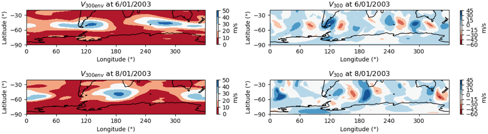
Figure 1.
Composite map of V300env (left figures) and V300 (right figures) during Rossby wave packets propagation.
Example 2: Hovmoller diagram of V300env during the propagation of Rossby wave packets: in this example we display the evolution of V300.and V300env in a Hovmoller diagram during the propagation of a Rossby Wave Packet. Figure 2 displays the evolution of V300 (Figure 2a), V300env (Figure 2b) and filtered V300env (Figure 2c) in the longitudinal section between mid latitudes (40–65°S) from the 6th to the 26th of January of 2003. As in Figure 1, we can observe the manifestation of troughs and ridges during the propagation of Rossby wave packets and the V300env captures it. Nevertheless, as we previously stated, it is difficult to track Rossby wave packets in Figure 2b if we do not filter out the noise. Hence, in Figure 2c we present the same diagram as in Figure 2b, but filtering V300env values below 19 m/s (as in Perez et al., 2021). As expected, it is now much easier to observe where these packets appear, their propagation, as well as the areas where they lose their stability and disappear.
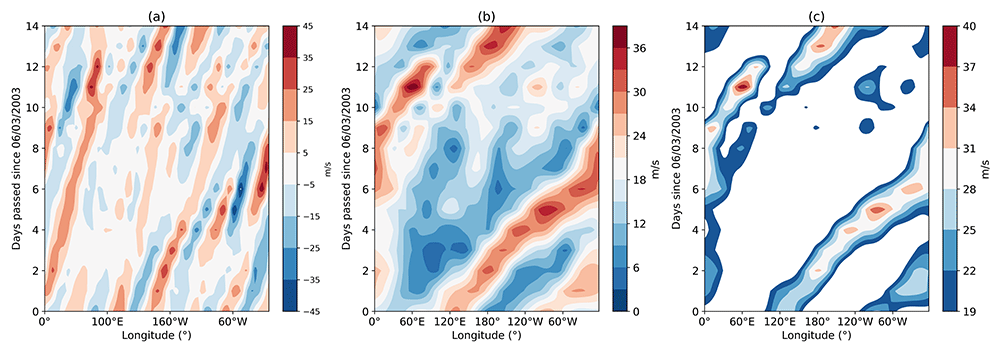
Figure 2. Hovmoller diagram of the temporal evolution of V300 (left figure), V300env (middle figure) and V300env (right figure) above the threshold of 19 m/s, (as in Perez et al., 2021), between 40–65°S.
Limitations
As we mentioned earlier in the document, this methodology requires that the Rossby wave packets travel mainly in the zonal direction, and this pattern is only observed during southern hemisphere summer (Chang, 1999). As a result, the datasets only covers the time period in which this methodology is effective to observe these atmospheric waves, which is the austral summer of the southern hemisphere
Data availability
Underlying data
Zenodo: Wind envelope at 300 hPa in the Southern Hemisphere during austral summer between 1979–2020. https://doi.org/10.5281/zenodo.7341912, (Pérez, 2021)
This project contains the following underlying data:
- V300_env_1979_2020_ERA_5_v1.1.nc (V300env data from December 1979 to March 2020 obtained using V300 ERA 5 data).
- V300_env_1979_2020_NCEPDOE2_v1.1.nc (V300env data from December 1979 to March 2020 obtained using V300 NCEP-DOE2 data)
The described data is available in a NetCDF-4 format
Data are available under the terms of the Creative Commons Attribution 4.0 International license (CC-BY 4.0).
Faculty Opinions recommendedReferences
- Chang EKM:
The Impact of Wave Packets Propagating across Asia on Pacific Cyclone Development.
Monthly Weather Review.
2005; 133(7): 1998–2015. Publisher Full Text
- Chang EKM:
Characteristics of wave packets in the upper troposphere. Part II: Seasonal and hemispheric variations.
J Atmos Sci.
1999; 56(11): 1729–1747. Publisher Full Text
- Grazzini F, Vitart F:
Atmospheric predictability and Rossby wave packets.
International Journal of the Royal Meteorological Society.
2015; 141(692): 2793–2802. Publisher Full Text
- Hans H, Bell B, Berrisford P, et al.:
The ERA5 global reanalysis.
R Meteorol Soc.
2020; 146(730): 1999–2049. Publisher Full Text
- Kanamitsu M, Ebusuzaki W, Woollen J, et al.:
NCEP-DOE AMIP- II Reanalysis (R-2).
Am Meteorol Soc.
2002; 83(11): 1631–1644. Publisher Full Text
- O’Brien L, Reeder JM:
Southern Hemisphere Summertime Rossby Waves and Weatherin the Australian Region.
Q J R Meteorol Soc.
2017; 143(707): 2374–2388. Publisher Full Text
- Pérez I, Barreiro M, Masoller C:
ENSO and SAM influence on the generation of long episodes of Rossby wave packets during southern hemisphere summer.
J Geophys Res Atmos.
2021; 126(24): e2021JD035467. Publisher Full Text
- Perez I:
Wind envelope at 300 hPa in the Southern Hemisphere during austral summer between 1979-2020 (1.1) [Data]. Zenodo. 2021. http://www.doi.org/10.5281/zenodo.7341912
- Pérez I:
Python script to measure wind envelope from meridional wind speed (1.0). [Code].
Zenodo.
2021a. http://www.doi.org/10.5281/zenodo.5724657
- Rossby CG:
On the propagation of frequencies and energy in certain types of oceanic and atmospheric waves.
J Meteor.
1945; 2(4): 187–204. Publisher Full Text
- Sagarra R, Barreiro M:
Characterization of extratropical waves during summer of the Southern Hemisphere.
Meteorologica.
2020; 45: 63–79. Reference Source
- Schulzweida U:
CDO User Guide (2.1.0).
Zenodo.
2022. Publisher Full Text
- Skansi MM, Brunet M, Sigró J, et al.:
Warming and wetting signals emerging from analysis of changes in climate extreme indices over South America.
Glob Planet Change.
2013; 100: 295–307. Publisher Full Text
- Souders MB, Colle BA, Chang EKM:
The climatology and characteristics of Rossby Wave Packets using a feature-based tracking technique.
Mon Weather Rev.
2014a; 142(10): 3528–3548. Publisher Full Text
- Souders MB, Colle BA, Chang EKM:
A Description and Evaluation of an Automated Approach for Feature-Based Tracking of Rossby Wave Packets.
Mon Weather Rev.
2014b; 142(10): 3505–3527. Publisher Full Text
- Stott AP, Christidis N, Otto LEF, et al.:
Attribution of extreme weather and climate-related events.
Wires Clim Change.
2016; 7(1): 23–41. Publisher Full Text
- Trenberth EK:
Observed Southern Hemisphere Eddy Statistics at 500 mb: Frequency and Spatial Dependence.
J Atmos Sci.
1981; 38(12): 2585–2605. Publisher Full Text
- Wirth V, Riemer M, Chang EKM, et al.:
Rossby wave packets on the Midlatitude waveguide- a review.
Mon Weather Rev.
2018; 146(7): 1965–2001. Publisher Full Text
- Zimin AV, Szunyogh I, Hunt RB, et al.:
Extracting envelopes of Nonzonally Propagating Rossby wave packets.
Mon Weather Rev.
2006; 134(4): 1329–1333. Publisher Full Text
- Zimin VA, Szunyogh I, Patil JD, et al.:
Extracting envelopes of Rossby wave packets.
Mon Weather Rev.
2003; 131(5): 1011–1017. Publisher Full Text