Implementation: the model under the package
All the equations and algorithms to model the benefits of urban agriculture were encapsulated in an R package (R Core Team, 2022), using one function for each indicator and one function to create scenarios. The package was created using R version 4.2.1 (R Core Team, 2022) in RStudio desktop v. 2022.07.02. The package structure was assisted by the package devtools (Wickham et al., 2022d) following the principles in Wickham and Bryan (2022a). Likewise, the documentation of the functions was assisted by the package roxygen2 (Wickham et al., 2022b). The dependencies of the package are:
Urban representation of the city of interest. The ediblecity package provides eight functions to estimate eight different indicators and a function to generate scenarios. It takes, as a basis, a spatial representation of a city (or a part of a city) as a GIS layer. This representation must have one attribute indicating the land uses of the city, such as gardens, streets, rooftops, etc. Some indicators require specific information to be included in the representation. This is explained in each indicator’s section.
The package includes the representation of Sant Narcís, a neighbourhood of Girona (Spain) as an example of an urban representation (Figure 1). This example can help the users to create the representation of their cities of interest. In the Table 1 below, a sample with one element of each type is shown. The representation is provided as an sf object, which is a class for spatial data in R implemented by package sf (Pebesma, 2018b)
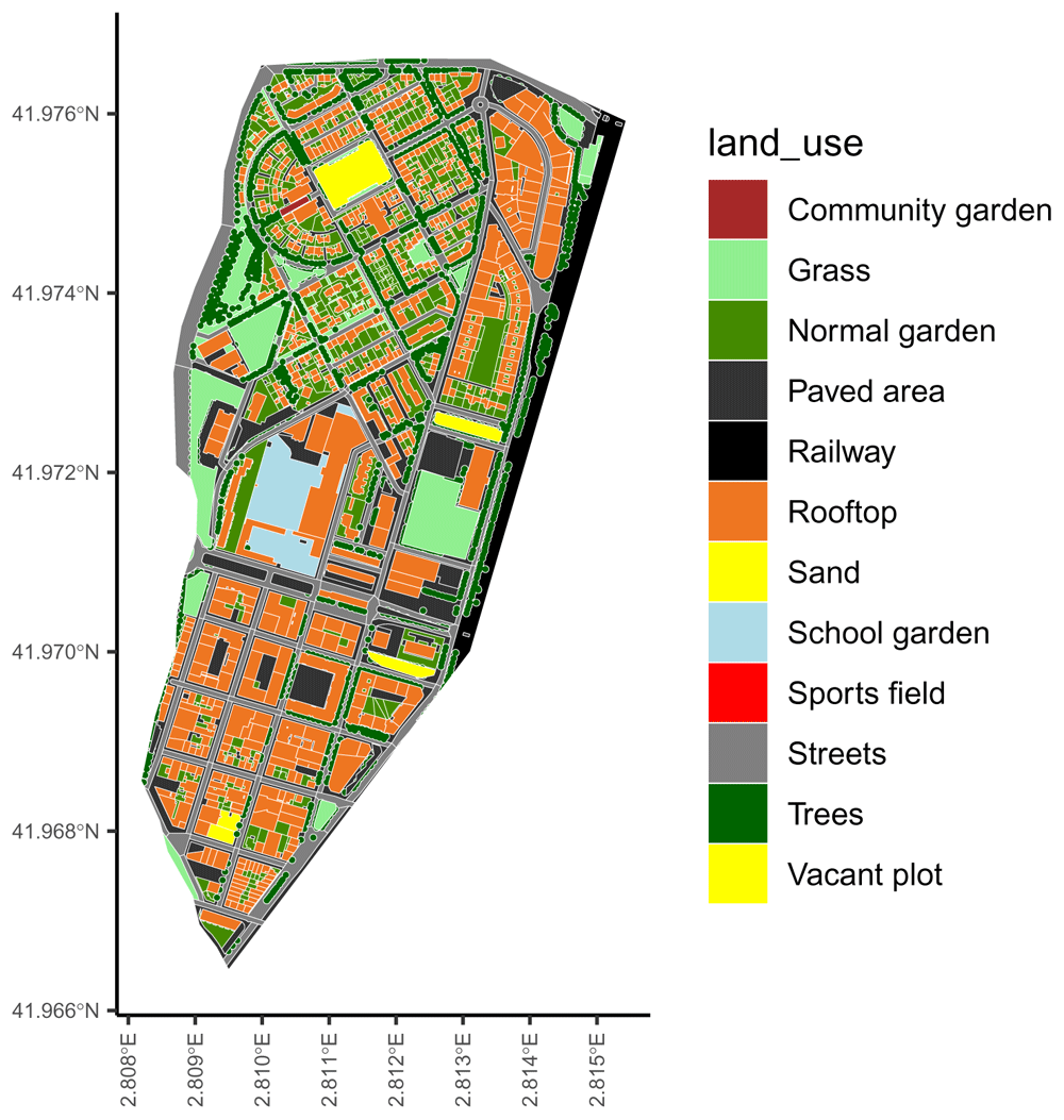
Figure 1. The urban representation included in the ‘ediblecity‘ package as example.
Table 1. Structure of the urban representation example.
| Column | Description |
|---|
| land_use | A category representing the urban elements |
| land_use_verbose | A more detailed category for the element, for example, if it is residential |
| floors | The number of floors of the element, 0 for non-built |
| area | The surface of the element |
| flat_area | The surface of the element that is flat (slope < 5⍛) |
| edible_area | The surface that is used to grow edible plants. Only applicable to urban agriculture solutions |
Along with the example for an urban representation, the ediblecity package also includes a data.frame with the default attributes of each green typology in the urban representation used to estimate the indicators (Table 2). This includes types of urban agriculture along with other types of green infrastructure. However, the user can provide their own attributes to estimate any indicator. In city_land_uses there are other columns not shown in Table 2, they are logical variables (i.e. TRUE/FALSE) used internally by the package to select urban agriculture elements.
Table 2. General attributes of the elements of urban green used to estimate the indicators.
| land_uses | pGreen | no2_seq1 | no2_seq2 | food1 | food2 | CN1 | CN2 |
|---|
| Edible private garden | 0.6 | 0.07 | 0.09 | 0.2 | 6.6 | 85 | 88 |
| Community garden | 1.0 | 0.07 | 0.09 | 0.2 | 2.2 | 85 | 88 |
| Commercial garden | 1.0 | 0.07 | 0.09 | 4.0 | 6.6 | 85 | 85 |
| Rooftop garden | 1.0 | 0.07 | 0.07 | 0.2 | 2.2 | 67 | 88 |
| Hydroponic rooftop | 1.0 | 0.07 | 0.07 | 9.0 | 19.0 | 98 | 98 |
| Arable land | 0.6 | 0.00 | 0.07 | 4.0 | 6.6 | 85 | 88 |
| Normal garden | 0.6 | 0.07 | 0.07 | 1.0 | 1.0 | 74 | 86 |
| Permanent crops | 0.6 | 0.09 | 0.09 | 4.0 | 6.6 | 65 | 77 |
| Vacant | 1.0 | 0.07 | 0.09 | 1.0 | 1.0 | 74 | 87 |
| Grass | 1.0 | 0.07 | 0.07 | 1.0 | 1.0 | 74 | 86 |
| Mulcher | 1.0 | 0.00 | 0.00 | 1.0 | 1.0 | 88 | 88 |
| Raised bed | 1.0 | 0.07 | 0.07 | 1.0 | 1.0 | 67 | 88 |
| Trees | 1.0 | 0.11 | 0.11 | 1.0 | 1.0 | 70 | 77 |
| Vegetated pergola | 1.0 | 0.07 | 0.07 | 1.0 | 1.0 | 98 | 98 |
pGreen is the proportion of green of the urban element. In urban agriculture solutions, this is overridden by the attribute edible_area. The following attributes come in pairs (min, max) to consider uncertainty in the estimations. The functions use a random value within the range provided by the pair of values for each element in the city. no2_seq is the capacity of the element to capture NO2 in gr/s. food is the food productivity in kg/m2 and CN is their curve number, used to calculate infiltration rates. The details are provided in following sections.
Indicators estimated. Urban heat island The urban heat island is a measure of how urban agriculture can contribute to climate change adaptation, specifically to adapt cities to the increasing heat waves (Langemeyer et al., 2021b). The indicator uses the equation developed by Theeuwes et al. (2017), which was validated in 14 cities. It calculates the difference in air temperature between the urban street canyon and the rural environment. To calculate this indicator, the user must provide a raster representing the sky view factor (SVF), which describes the proportion of the unobstructed hemisphere above a certain location. SAGA, a collection of open-source algorithms for geocomputation, provides an algorithm to calculate the SVF (Conrad, 2008).
where Fveg is the proportion of vegetation in cell i; Qql is the daily average global radiation (in W/m2/hour); Cair is the air heat capacity (in J); Pair is air density (in kg/m3); ∆T is the difference between the maximum and minimum daily average temperatures (in ⍛C); and U is the daily average wind speed (in m/s).
The indicator to estimate the urban heat island is implemented by the package under the function UHI (code snippet 1). The user must provide the urban representation (x) and the raster with SVF values (SVF). The green_df argument is a data.frame with the proportion of green of each land_use in the urban representation (Fveg in the equation). All the meteorological arguments are provided by default, based on the example provided (Mediterranean climate). However, the user can override them to provide values of their city of interest.
The function returns by default a summary of statistics of the UHI in x (min, 25%, 50%, mean, 75% and max values). If the argument return_raster is set to TRUE, the function returns a raster as stars object (Pebesma, 2021) with the UHI values. If verbose is set to TRUE, then the function returns a vector (i.e. an array) with the UHI in each cell. Both use the same resolution than SVF.
Code snippet 1: Function and arguments to estimate urban heat island.
UHI(
  x,                              # Urban representation
  SVF,                           # Raster with the sky view factor
  green_df = NULL,             # Fveg in the UHI equation
  Qql = 6.11,                   # Daily average global radiation
  Cair = 1007,                  # Air heat capacity
  Pair = 1.14,                  # Air density
  Tmax = 30.8,                  # Maximum daily average temperature
  Tmin = 20,                    # Minimum daily average temperature
  windspeed = 2.77,            # Average wind speed
  return_raster = FALSE,      # Should function return a raster or numeric values?
  verbose = FALSE              # Should the function return all the values or a summary?
)
Runoff prevention Surface runoff is the flow of water occurring on the ground surface when excess rainwater can no longer sufficiently rapidly infiltrate in the soil. Hence, runoff mitigation contributes to climate resilience since rain events will increase due to climate change (Shukla et al., 2019). The indicator measures the runoff in the city after a specific 24-hours rain event as well as the amount of rainwater harvested by harvesting systems. We departed from the model developed by the Soil Conservation Service (USDA), known as SCS runoff curve number method (Cronshey et al., 1985).
where Q is the runoff in mm; P is the rainfall volume in mm; Ia is the initial abstraction (all losses before runoff begins); and S is the potential soil moisture retention, which is a function of the curve number (which is determined by hydrologic soil group, see Cronshey, Roberts, and Miller (1985) for more details on the method). The SCS generalizes Ia as 0.2S, we modified this generalization to include the rainwater harvested:
where Rh is the potential water harvested by the element i, calculated as the amount of water fallen on the surface of adjacent higher buildings that are not used for gardening (in litres); Ws is the water storage capacity of the element i in terms of tank volume (in litres). From both, the minimum is used to calculate Ia.
The runoff_prev function estimates the runoff (Q in the equation) as well as the total rainfall in x and the total rainwater harvested in cubic meters (code snippet 2). Along with the urban representation (x), the user must provide a data.frame (runoff_df argument) with four variables: land use, minimum and maximum curve numbers and a logical variable indicating whether the land use (a urban garden, a building,. . . ) has potential to harvest rainwater. The argument rain allows to set the rain event (in mm), which must be defined by the user. The curve number of each element is randomized within this range provided in runoff_df. If runoff_df is not provided, city_land_uses is used instead. Following, floors_field is the name of attribute in x that specifies the number of floors of each element; harvest_dist (in m) is the maximum distance to consider that a building is adjacent to the element; and tank_size is a range for the volume of the rainwater tank, proportional to the surface of the element (in l/m2). The volume of each tank in the city is randomized within this range and multiplied by the element where they are located. All randomizations follow a random uniform distribution within the correspondent range.
Code snippet 2: Function and arguments to estimate runoff prevention
runoff_prev(
  x,                              # Urban representation
  runoff_df = NULL,             # A data.frame with land use values
  rain = 85,                     # Rain event in mm.
  floors_field = "floors",     # Variable in `x` containing the number of floors of each element
  harvest_dist = 10,            # Maximum distance to consider for rainwater harvesting surfaces
  tank_size = c(0, 45)          # Range for the size of tanks in m3
)
Green areas accessibility This indicator calculates the distance from each home to the closest public green area and return a summary of statistics (min, 25%, 50%, mean, 75% and max). It includes the possibility to exclude areas smaller than a threshold. The function to calculate these distances is green_distance (code snippet 3). It requires, as usual, the urban representation (x) and a vector with all the categories considered public green areas. If it is not provided, the function uses the categories from city_land_uses where the attribute public is TRUE. The argument residence_col indicates the variable of the urban representation (x) that must be used to identify the residences. Subsequently, residences indicates which categories of the ones contained by the variable passed to residence_col must be considered. The min_area argument can be used to exclude smaller areas than the value passed to the function (the threshold mentioned above).
If percent_out is set to TRUE, the function returns the percentage of houses that are further than max_dist argument from their closest public green area (excluding areas smaller than min_area). The default values for min_area and max_dist follow the recommendations of the World Health Organization, who recommended that all residences should be closer than 300 meters from a public green area larger than 0.5 ha.
Finally, if verbose argument is set to TRUE, a vector with all distances from residences to green areas (larger than min_area) is returned.
Code snippet 3: Function and arguments to calculate green accessibility
green_distance(
  x,                                           # The urban representation
  green_cat = NULL,                          # The land uses considered urban green
  residence_col = "land_use_verbose",     # The variable than contains information of what is a residence
  residences = "Residence",                 # The categories of former variable considered residences
  min_area = 5000,                           # Smaller areas are not included in the calculations
  percent_out = FALSE,                      # Should the function return a percentage of residences out
  max_dist = 300,                            # Which is the distaince to consider that a residence is out?
  verbose = FALSE                            # Should return a summary of distance or all values?
)
Nitrogen dioxide sequestration Nitrogen dioxide is a good proxy of overall air quality (Mayer, 1999) and one of the most concerning issues in cities, with important consequences on respiratory diseases and lung cancer (Kampa & Castanas, 2008). This indicator calculates the amount of NO2 sequestered by urban green and urban agriculture solutions (in g/s).
where ai is the area (in m2) of the element i; and capi is the capacity of element i to sequester NO2 (in µg·s-1m-2).
The function to estimate the NO2 sequestered is no2_seq (code snippet 4). It has only two arguments; the urban representation (x) and a data.frame with four columns:
land_uses: Column with the land use.
no2_seq1: The low range of NO2 sequestration of each function (in µg·s-1m-2).
no2_seq2: The high range of NO2 sequestration of each function (in µg·s-1m-2).
pGreen: The proportion of green surface in each function.
When the argument is NULL (default), the function uses the city_land_uses dataset provided with the package that contains NO2 sequester capacity of different types of urban green.
The capacity (capi in the previous equation) of each element is randomized within the range provided by no2_seq1 and no2_seq2. As well the area of each element is multiplied by pGreen. In urban agriculture solutions, the attribute edible_area overrides the more general pGreen.
Code snippet 4: Function and arguments to calculate NO2 sequestration
no2_seq(x,                     # The urban representation
         green_df = NULL)     # The data.frame with the NO2 sequestration capacity of each land use.
Jobs created and volunteers involved When the urban agriculture solutions are community solutions they need volunteers to be involved. On the other hand, when they are for commercial purposes, they are supposed to create jobs. Therefore, two indicators are proposed to account for the hours of work in the ECS. One indicator relates to volunteers’ time and the other one relates to time spent by new workers (jobs created). Both indicators use the same equation:
where ai is the area in m2 used to grow plants (edible_area) in the element i; and k is the number of jobs or volunteers by m2. In both functions, k is sampled from a random uniform distribution within the specified range. Then, a Monte Carlo simulation of 1,000 iterations is executed to estimate the confidence interval. The default values were based on two sources, an empirical study (CoDyre et al., 2015) and the FoodMetres project.
The functions to calculate these indicators are edible_jobs and edible_volunteers respectively (code snippet 5). They share the same arguments, expect for jobs and volunteers, which is the value of k in the previous equation. As usual, the first argument is the urban representation (x), edible is the land uses in x that are urban agriculture solutions (if NULL, city_land_uses is used as default), the attribute of x defining the area used to grow plants is area_col, the confidence interval is defined in interval, and if verbose is set to TRUE, instead of the confidence interval, the function returns a vector of length 1,000 with all the results of the Monte Carlo simulation.
Code snippet 5: Function and arguments to calculate number of jobs created and volunteers involved in urban agriculture.
edible_jobs(
  x,                                    # The urban representation
  jobs = c(0.000163, 0.022),         # The k parameter
  edible = NULL,                      # The land uses that are urban agriculture
  area_col = "edible_area",          # The variable containing the surface dedicated to grow plants
  interval = 0.95,                    # The confidence interval returned by the function
  verbose = FALSE                     # Should return all values or a summary?
)

edible_volunteers(
  x,                                    # The urban representation
  volunteers = c(0.00163, 0.22),    # The k parameter
  edible = NULL,                      # The land uses that are urban agriculture
  area_col = "edible_area",          # The variable containing the surface dedicated to grow plants
  interval = 0.95,                    # The confidence interval returned by the function
  verbose = FALSE                     # Should return all values or a summary?
)
Green per capita We propose an indicator to estimate green per capita at neighborhood level and at city level, including public and private gardens to account for environmental justice (Kabisch & Haase, 2014). At the neighborhood level a ratio between the most and least green neighborhoods is calculated, with higher values meaning a major difference between neighborhoods and less spatial justice. Moreover, since wealthier areas tend to have more private gardens (Farahani et al., 2018), these can be included in the account of green per capita to not underestimate green per capita in those neighborhoods.
The function to calculate this indicator is green_capita (code snippet 6). Along with the urban representation (x). As in other functions, the green_categories argument in the function is a list of the categories to be considered as green areas. To calculate the green per capita in the overall city, the user must provide the number of inhabitants in inhabitants. At a city level, the function returns the average amount of green per capita in the city (in m2/inhabitant). Likewise there are two options to calculate green per capita at a neighbourhood level. The urban representation can contain two variables indicating the name of the neighbourhood and the inhabitants (specified in name_col and inh_col arguments respectively). Or the user can provide a GIS layer with the neighbourhoods’ boundaries and their attributes.
Furthermore, when the private argument is set to TRUE, the private gardens are also considered. Alternatively, the user can provide a list of elements to be considered as private green areas (e.g. parks, urban gardens,. . . ). When the argument verbose is set to TRUE, the function returns the green per capita in each neighbourhood instead of the ratio between the most and least green ones. Finally, the argument min_inh is to exclude neighbourhoods whose number of inhabitants is under a threshold to avoid the bias in green per capita due to unpopulated neighbourhoods (e.g. industrial districts).
Code snippet 6: Function and arguments to calculate green per capita.
green_capita(
  x,                            # The urban representation
  green_categories = NULL,   # The categories considered as urban green
  inhabitants = NULL,         # The number of inhabitants in the city
  neighbourhoods = NULL,      # The spatial representation of neighborhoods
  name_col = NULL,             # The variable that contains de name of the neighborhoods
  inh_col = NULL,              # The variable that contains the inhabitants of the neighborhoods
  private = FALSE,             # Should private green be considered?
  verbose = FALSE,             # Should return all the information or just the ratio?
  min_inh = 0                   # Neighborhoods with less hanbitants are excluded
)
Food production Although many authors stated that the main goal of urban agriculture is not to produce food (Säumel et al., 2019; Tornaghi, 2012), food production is undoubtedly an important component of urban gardens (Furness & Gallaher, 2018; Steel, 2008) and the most frequent output modeled at a city scale (Grafius et al., 2020; Grewal & Grewal, 2012). The food production is measured in terms of productivity (kg/m2):
where yk is the yield (in kg/m2) of the category k of urban garden; and ai is the area of urban garden i in m2. By default, the value of y is randomized using a random uniform distribution within the range defined by food1 and food2 values in city_land_uses, which are the minimum and maximum yield values found in the literature for each category of urban garden. The function computes a Monte Carlo simulation of 1,000 iterations to calculate the confidence interval.
The function that calculates the food production is food_production (code snippet 7). It takes the urban representation (x) as the first argument. If the second argument edible_df is NULL, the function uses the values from city_land_uses as specified above. Otherwise, the user can provide its own values as a data.frame with three columns:
land_uses: specifying the category of urban agriculture, it should match the categories from x.
food1 and food2 specifies the range of the random uniform distribution to randomize yield.
The argument area_col points to the variable of x that determines the area dedicated to grow plants in each urban garden. If NULL, the total area of each element is used instead. The number passed to interval defines which confidence interval of the food production must be returned by the function. However, if verbose is set to TRUE, the function returns a vector of length 1,000 with the results of each iteration of the Monte Carlo simulation.
Code snippet 7: Function and arguments to estimate food production
food_production(
  x,                           # The urban representation
  edible_df = NULL,          # Dataframe containing information on yields
  area_col = "edible_area", # Variable of x with surface
  interval = 0.95,           # Confidence interval returned by the function
  verbose = FALSE            # Should return all the values or just the confidence interval?
 )
Scenarios of urban agriculture. The ediblecity package also provides the user with a function to create new scenarios based on the urban representation and a predefined set of urban agriculture solutions (Table 3) based on where they are located (private gardens, plots on ground or rooftops) and their purpose (private, community or commercial). The function returns a spatial representation of the new scenario (sf object) with the same structure of the urban representation.
Table 3. Elements created in new scenarios.
| Urban agriculture solutions | Location | Purpose |
|---|
| Edible private garden | Private gardens | Private |
| Community garden | Plots on ground | Community |
| Commercial garden | Plots on ground | Community |
| Rooftop garden | Rooftops | Commercial |
| Hydroponic rooftop | Rooftops | Commercial |
The location of new urban agriculture elements is randomized among all locations that fulfill the requirements of minimum area for that element. However, this is not the case for commercial gardens, they are settled in the larger available locations, assuming that commercial initiatives have the power to acquire the best spots.
The function to create a new scenario is called set_scenario (code snippet 8). It requires many arguments but most of them have default values to facilitate its use. The function needs the urban representation (x). Then three arguments (pGardens, pVacant, pRooftop) control the proportion of new elements that must be created. The next three arguments (edible_area_*) control the proportion of the area of the new elements that is dedicated to grow plants (edible_area). The edible_area of each new elements is randomized within the range provided in the arguments. The next trio of arguments (min_area_*) specify the minimal area required to create new elements. If there are not enough elements larger than min_area_* to fulfill the first arguments, a message is displayed to inform the user (unless quiet argument is set to TRUE). Another three arguments (*_from) control which elements can be converted from the urban representation to create new urban agriculture solutions. The argument pcommercial controls the percentage of plots on ground and rooftop that should have commercial purposes instead of community. This does not affect private gardens since they are assumed to be for personal use. Finally, area_field specifies which attribute of x must be used as the area of the elements. By default, it is am attribute called flat_area that measures the area with an slope lower than 5⍛ (in city_example).
Code snippet 8: Function and arguments to create new scenarios.
 set_scenario(
   x,                                               # The urban representation
   pGardens = 1,                                  # Proportion of private edible gardens
   pVacant = 1,                                   # Proportion of vacant plots converted to gardens on ground
   pRooftop = 1,                                  # Proportion of rooftops converted to rooftop gardens
   edible_area_garden = c(0.02, 0.3),          # Proportion of surface dedicated to grow plants in private gardens
   edible_area_vacant = c(0.52, 0.75),         # And in gardens on ground
   edible_area_rooftop = c(0.6, 0.62),         # And in rooftop gardens
   min_area_garden = 10,                         # Exclude smaller private gardens
   min_area_vacant = 100,                       # Exclude smaller vacant plots
   min_area_rooftop = 100,                      # Exclude smaller rooftops
   private_gardens_from = "Normal garden",    # Land uses to be converted to private edible gardens
   vacant_from = "Vacant",                      # Land uses to be converted to gardens on ground
   rooftop_from = "Rooftop",                   # Land uses to be converted to rooftop gardens
   pCommercial = 0,                              # Proportion of commercial gardens vs community gardens
   area_field = "flat_area",                   # Variable of x containing available surface in each element
   quiet = FALSE                                 # Should the function raise warnings?
)








