Introduction
Currently, one of the major targets of governments and policy makers world-wide is the reduction of the greenhouse gas (GHG) emissions worldwide to meet the Paris climate targets to curtail the further temperature increase to 1.5° up to 20501. The use of energy globally contributes by about 75% to the total GHG emissions. Hence, one of highest priorities, in order to reduce GHG emissions, is to implement appropriate policy measures in the energy sector as immediately as possible. To reduce energy consumption, the most effective and suitable policies and measures to assist in meeting the limiting temperature increases targets up to 2050 and heading toward sustainable energy systems have to be identified. An additional motivation for the research conducted in this paper is to identify the impact of so-called discontinuities.
Reliable modelling of an energy system, including development of different scenarios, is of core relevance to identify possible pathways for decarbonisation of any energy system in any geographical area world-wide. Regarding modelling of energy systems, the logic is simply as follows: first, future energy demand has to be modelled and then, secondly, the supply side because if there is no demand, there is also no need for modelling a supply side of the system providing energy for the consumers in the different sectors. On the supply-side it will be modelled how the estimated energy demand can be provided in an optimal way, e.g. with lowest possible costs. Energy demand needs to be modelled depending on the impacts of policies, in static as well as in dynamic models. The supply side of the energy systems is to be modelled usually by means of optimization and simulation approaches.
An important category that has recently gained importance according to this HORIZON project and that can be considered qualitative as well as quantitative is open-source modelling. Especially, in the field of supply side analysis of energy systems open-source modelling has become increasingly established, including all aggregation levels of the supply side and various optimisations as well as simulation model approaches see e.g., Despres et al.2 and Prataviera et al.3. The major advantage of open-source modelling is the transparency of approaches and data used. It can be described based on the FAIR principles (Findable, Accessible, Interoperable, Reusable).
The FAIR Data Principles (Findable, Accessible, Interoperable, and Reusable), published in Scientific Data in 2016, are a set of guiding principles proposed by a consortium of scientists and organizations to support the reusability of digital assets. These principles have since been adopted by research institutions worldwide. The guidelines are timely as we see the unprecedented volume, complexity, and speed in creation of data.
The core objective of this paper is to carry out a review of econometric energy demand modelling approaches in a historical context over the past about 50 years to better understand its status quo. Of specific interest is to analyse what has changed over time regarding statistical approaches used. In addition, we have investigated how the results for price and income elasticities have changed, especially, whether static approaches are still useful or dynamic ones are preferable. Finally, the consequences for energy policy are discussed.
In this context, special attention is paid to lessons learned from modelling historical discontinuities and structural breaks in order to better understand the recent developments related to COVID19. That is to say, not the effects of the pandemic itself are investigated but how to consider discontinuities, disruptions and structural breaks due to “unexpected influences from outside” in principle. We consider whether these unexpected short-term disruptions really require new or additional modelling elements, or whether they can simply be represented by well-known influence parameters, such as income, consumer spending or economic output (i.e., Gross domestic product (GDP)) or short-term behavioural changes associated with longer-term reversion to habitual patterns of energy consumption. The final objective is to identify the key consequences for policymakers by defining the most effective types of policies for curbing carbon emissions in the energy sector and straightforwardly mitigating global warming.
In principle, this paper combines a mixture between a historical review paper with some exemplary analyses presenting a technical paper. The main novelty of this paper is, that – to the best of our knowledge – it is the first to analyse and document the following three issues simultaneously: (i) the historical development of econometric energy demand modelling approaches providing exemplary results for the example of oil demand in selected regions in a systematic way, (ii) exemplifying how the dynamics of elasticities developed over time and (iii) emphasis and analyses of the effect of discontinuities and structural breaks.
The paper is organized as follows: after presenting and acknowledging the historical literature and, subsequently, exploring the different approaches of energy demand modelling in the following sections. Our methodological approach is explained after the brief history. It starts with the basics and definitions of “energy modelling” to understand the connections and relations between modelling of energy systems, energy demand, energy supply and energy policies. We then examine the role of (irreversible) efficiency improvements and the historical maximum prices are described and analysed for the specific example. The subsequent section focusses on the dynamics of elasticities and depicts the specific developments in the chosen example of oil demand in three world regions as described in section “methods”. The impacts of structural breaks and disruptions are investigated, and the final section presents our analysis of which major energy policy instruments exist to interfere. Conclusions complete the work.
A brief review of the history of energy demand modelling
In the last five decades different approaches for econometric modelling of energy demand were developed but in principle all were based on modelling energy demand depending on income and price elasticities. Moreover, scenarios for future energy demand are derived considering assumptions regarding the future development of the most important economic parameters such as energy prices or GDP, see e.g., Pindyck/Rubinfeld4, and Ryan/Plourde5.
Since the 1970s different stages of modelling energy demand are observed and can be divided into two categories:
1. Qualitative discussion:
new parameters entering the modelling scene step by step, e.g., price, historical maximum price, error-correction-term; some parameters were disappearing, e.g., the symmetric koyck lag, yet from our point-of-view most important is the question whether approaches assuming constant elasticities over time are or time-dependent elasticities are used.
2.Quantitative development (not necessarily improvement) of mathematic statistical tools, e.g. Cointegration, Autoregressive Distributed Lag (ARDL)). This issue is linked to significant improvements in computer capacities over time.
The story starts in the early 1970s. After the member countries of the Organization for Economic Co-operation and Development (OECD) experienced considerable increases in energy demand during the decade 1960–1970, the consequences led to the first oil crises in 1973/74. After 1973, energy consumption has been growing much more moderately, likely caused by a slowdown in economic growth rates and an increase in real energy prices. To mark this moment, in 1972, Meadows6 published his seminal contribution on “The Limits to Growth”, announcing resource shortages and increasing prices.
While before 1973 energy demand was simply modelled as a linear function of income, a more differentiated development took place afterwards. It started with including prices in the former solely income dependent models. The turbulences in the world oil price in the 1970s led to the emergence of a new culture in modelling energy demand. Pindyck/Rubinfeld4 provided the first comprehensive work on the structure and analysis of world energy demand. Pindyck7 conducted one of the first and most comprehensive analyses on price and income elasticities by fuel type. Kouris8 published the paper “Elasticities - Science or Fiction?” in 1981. He argued that there are some severe problems presented by using constant elasticities only. Madlener9 was one of the first to provide a systematic approach, analysing the strengths and weaknesses of various demand approaches - considering the bottom-up as well as the aggregated dimensions. Already in in 1996, he pointed towards the problem of missing ex ante approaches for energy demand modelling.
After the drop in oil prices in the mid-1980s discussions focused on irreversible technological efficiency improvements leading to asymmetric demand reactions, and studies focusing on the impact of historical maximum prices were conducted by Gately10,11 and Dargayand12. Walker and Wirl13 analysed the transport sector and concluded that irreversible efficiency improvements such as cars with lower specific gas consumption were the major reason for the moderate rebound in oil demand after 1985. For a more recent work on the oil issue see Gallo14. Haas and Schipper15 found significant evidence that technical efficiency is an important parameter for describing the evolution of residential energy demand.
Regarding the method over a long period of time, Ordinary Least Square (OLS) estimates were the dominating approach at least until about 1993. Engsted and Bentzen16 were among the first suggesting unit root tests for testing the stationarity of the depending variables, e.g., prices, in time series analyses and applying cointegration approaches for energy demand modelling. In the following years, a series of new approaches started considering step-by step asymmetries, lags, dynamics and finally structural breaks and disruptions. Ryan and Plourde5 provided one of the last comprehensive surveys on energy demand analyses in general, Ajanovic et al.17 for transport specifically. An extension of the basic approaches consisted of adding some form of dynamic adjustment mechanisms. Yet, it has proven difficult to extend the theoretically more rigorous approaches to include dynamic adjustment processes. For a further discussion of this issue with respect to transport see 18. Studies for different fuels in the residential sector were conducted in 19 and 20. For an application of energy demand modelling with respect to natural gas demand see 21 for modelling price relationships see 22. Some applications of energy demand modelling with respect to the German “Energiewende” can be found in 23 and 24.
Hanna and Gross25 provide a very comprehensive literature review on structural breaks and disruption in modelling energy demand. They explore, in their review, how different energy system models and scenarios explicitly represent and assess potential disruptions and discontinuities following definitions of disruptions and discontinuity set out by Burt26 which should help to distinguish between the two concepts and are consistent with Ayres’ expanded criteria for discontinuity27; for a meta-analysis of scenarios see Densing et al.28.
Finally, regarding the the COVID19 pandemic, the following references deal with the short-term observations (especially in terms of energy/electricity demand and CO2 evolution) There are review papers such as Krarti29 or Navon30, country-specific studies such as Malliet et al.31 and others, Dawud and Kemfert32, Jiang et al.33 and Cheshmehzangi34). However, they all can hardly contribute to a better understanding of longer-term impacts of energy demand patterns after an unexpected event. Corresponding empirical studies on quantitative effects can only be conducted in the future.
Methods
Despite being very often used, the term “energy modelling” is very imprecise, notwithstanding Albert Einstein’s formula E=mc². A more precise formulation for “energy modelling” is at least “energy system modelling” or, more strongly, from an energy economics perspective, “energy market modelling” or “energy policies modelling”. If the modelling of energy systems is specified more precisely, the models are split in energy supply and energy demand models (see Figure 1). At first, demand needs to be modelled then supply. The reason is simply, that if there is no determination of demand, there is no need to model the supply side. However, energy demand cannot be treated in isolation. The most important interactions with the supply side and energy policy within the energy system must be considered too.
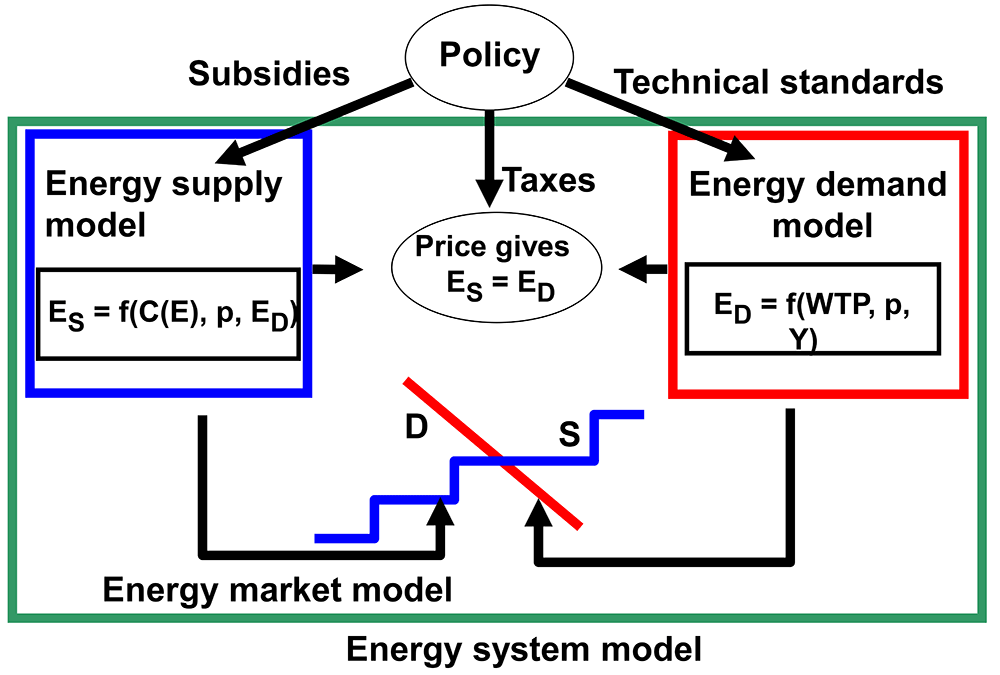
Figure 1. Basics of energy system modelling and the impact of price and income as well as different policy instruments such as subsidies, taxes and technical standards.
Figure 1 depicts the components of an energy system model. The model for energy demand ‘ED’depends on consumers’ willingness to pay ‘WTP’ as well as on the price of energy ‘p’ and the income ‘Y’. The model for energy supply ‘ES’ depends on the marginal production costs of energy ‘C(E)’, from the market price ‘p’ and on overall energy demand. Demand and supply model provide in their intersection of demand and supply the market price ‘p’ and the corresponding energy market equilibrium. In addition, different types of policies (e.g., subsides, taxes, technical standards) may interfere within the overall energy system model on the demand or supply side or as taxes on the price.
The method used in the following is based on econometric analyses. Econometric approaches are widely used for analyzing energy demand. We have conducted a thorough review of the peer-reviewed literature which is documented in the course of this chapter. The major reason behind choosing this approach is that it provides an insight on the magnitude of impact of different parameters such as income and energy prices as well as the analysis of possible structural breaks.
We reviewed how the econometric modelling approaches developed over time, and the most important corresponding equations are illustrated by applying it to an own example. The example is on modelling historical oil demand for the EU, the USA and the OECD. This example is chosen mainly due to the availability of empirical data, but also to the need to phase-out oil in order to decarbonise energy systems as quickly as possible. However, the methods and modelling approaches used in this paper can be applied equally to any energy carrier or sector e.g., electricity demand or transport/industrial sectors that are of particular interest for achieving the European 2030 (EU Green Deal) or 2050 climate neutrality targets. The formal analyses documented in this paper are mainly conducted for pedagogic reasons to exemplify how such analyses could be conducted. It is not our goal to conduct in-depth econometric analyses per se. but to provide some examples to illustrate the theory.
The inclusion and exclusion criteria for including the models/methods are that we have selected econometric approaches applied so far in the peer-reviewed literature and we have excluded all other approaches. The objective was to conduct assessments which of these econometric methods provide useful results and which do not.
Consequently, the documentation starts with the early purely symmetric approaches which emerged in the 1970s, looking next at asymmetries and irreversible efficiency improvements, as well as lags and disruptions/structural breaks. We also consider the development of widely used mathematical approaches over time such as cointegration. We end with two well-known and understood analytical approaches to identify disruptions and structural breaks in energy demand modelling in the past; the so-called “Dummy variables” and the “Chow-Test”. In the following exemplary analysis, the programme MICROFIT 5.5 created at Oxford university - which can be downloaded for free from the internet is used. With MICROFIT 5.5 we applied regression analyses choosing UNIVARIATE/single regression menu from the main page of the programme and choosing ordinary least-squares (OLS) approach. It was applied using the Equation (1) to Equation (6) documented in the following and leading to the results documented in Table 1.
Table 1. Estimates of static elasticities of long-term oil consumption over the period 1960 – 2020 using the ordinary least-squares (OLS) approach.
| EU-15 | OECD | USA |
|---|
| w/o lag | w/ lag | w/o lag | w/ lag | w/o lag | w/ lag |
|---|
| α (LT price elasticity) | -0.12 | -0.11 | 0.00 | -1.00 | 0.00 | -1.00 |
| β (LT income elast) | 0.38 | 0.22 | 0.40 | 1.25 | 0.30 | 0.50 |
| A (ST price elasticity) | -- | -0.01 | -- | -0.08 | -- | -0.04 |
| B (ST income elast) | -- | 0.02 | -- | 0.10 | -- | 0.02 |
| λ (lag) | -- | 0.91 | -- | 0.92 | -- | 0.96 |
| R2_corr | 0.49 | 0.99 | 0.64 | 0.99 | 0.65 | 0.97 |
The basic standard estimation approach for modeling energy demand by means of a production function, depending on price and income, is presented in equation one. This approach is also called a partial demand model (Pindyck/Rubinfeld4) because overall interactions of an economy are not considered. The equations used in the following are taken from Pindyck/Rubinfeld4, Walker/Wirl13, Ryan/Plourde5 and Ajanovic/Haas18. In the basic Equation (1), the dependent variable is energy demand Et, the explanatory variables are the energy price Pt with the price elasticity a and income Yt with the income elasticity β:
with:
C…………Intercept
Et……….. Energy demand in year t (non-climate-corrected)
Pt…..……. Real energy price (calculated by means of weighted fuel prices)
α ………....Long-term price elasticity
Yt…..……. Real income, e.g. Gross Domestic Product (GDP)
β………….Long-term income elasticity
In logarithmic form for making OLS estimates or other regression analyses possible is a sum such as:
where:
εt ……residual (error term)
The next question is whether lags in adaptation to changes in price and income exist. The reason is simply that consumers may respond in the short-term by means of changes in behaviour but in the long-term by means of investments e.g. in efficiency measures, such as building insulation or new and cleaner heating systems. This principle is depicted in Figure 2. It can be seen that there is a short-term response to price increases due to changes in behaviour e.g. in transport driving less and with some delay there is a more pronounced long-term effect, considering a possible change to a more efficient technology, e.g. in transport an energy-saving electric vehicle. If the appropriate decision and response period is sufficiently long, lagged explanatory variables should be included explicitly in the model. This is done in the following Equation (3) by including λ.
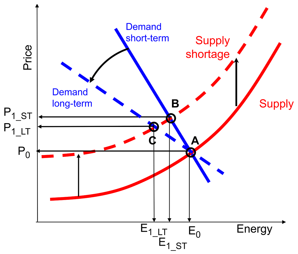
Figure 2. Short-term and long-term adaptation to changes in market prices for energy.
The basic equation in (1) is extended to:
with:
λ .......... „Lag“
And in logarithmic form:
where:
A= Short-term price elasticities, B= Short-term income elasticities
The lag λ is a relative delay but can be translated e.g. into years. If λ is 0.5, for example, it means that the lag in years is 1/(1-0.5) = 2 years. Furthermore, it is also important to differ between long-term and short-term elasticities. While the short-term elasticities capture the immediate behavioural responses, the long-term elasticities capture the full changes over time including investments in efficiency or changes in modes in transport. This is the reason why short-term and long-term elasticities have been implemented. in the literature see e.g.Walker/Wirl (1993).The long-term elasticities are calculated by means of dividing short-term ones by (1-λ):
As already mentioned in the introduction, the chosen empirical example elaborates in the analysis of the historical oil demand. Table 1 depicts the result of exemplary estimates with and without a lag for EU-15, OECD and the USA over the period 1960–2020. The rationale why for the estimates in this paper data from 1960 to 2020 were used is that before 1960 no consistent data sets are available.
The methods used to collect the information were based on our knowledge of which organisations, institutions and companies that provide data in this context. The major sources identified for the data needed were:
BP35,OPEC36,
OECD37
World Bank38
Note, that no automation tools were used in this process. The reason why for Europe only EU-15 countries are considered is simply that these were the only European countries where the time series for GDP were available since 1960. In the first two lines of Table 1, the estimates of the long-term elasticities are documented. The values in the columns with lags are calculated using the Equation (5) and Equation (6). It can be seen that for OECD and USA the differences in the long-term price elasticities with lag are quite high (between (0.11) and 1) which is mainly caused by the large magnitude of the lag (> 0.9 for every country). The long-term price elasticities without lag are of low magnitude for all countries implying that, regarding the long-term income elasticities with and without lags, they are rather in the same range (in a range between 0.3 and 0.5, except for OECD, it is 1.25). Most interesting is that the lags are tremendously high and so are the R2 (Coefficient of Determination) in the estimates with lags.
A major final address of this paper will eventually be to identify whether the approaches assuming constant elasticities over time still provide any useful results. From the results of Table 1 the situation is still ambiguous but as demonstrated in the latter sections of our paper, a dynamic effect over time is observed which strongly questions this static approach.
Note, that the specific elements of the data sources cited are based on the Equation (4) to Equation (6). The specific parameters used for the estimates presented in Table 1 are
- Oil consumption E (Source: BP35)
- The oil price p (Source: BP35)
- GDP Y (Source: OECD37).
A specific category of approach is so-called cointegration. In some papers in the 1990s (e.g., Bentzen and Engsted16) it was argued, that so-called cointegration techniques could be an important tool for current and future analyses of energy demand and, might be a straightforward method for deriving energy policies. Cointegration means that a long-term equilibrium between the variables exists, see Malliet et al. (2021)31. For cointegration analyses different approaches exist, yet the ARDL (Autoregressive Distributed Lag) approach turned out to be most favourable, according to Pesaran&Pesaran (2015)39 especially because cointegration analyses can be conducted regardless of whether the variables are stationary or non-stationary. In this process we firstly analyze whether the variables in Equation (3) are cointegrated and if they are, an Error-Correction-Model (ECM) is applied to investigate long-term as well as short-term elasticities and the speed of adjustment. The major advantages of ECM are that they allow us to clearly distinguish between short-term and long-term elasticities, because both total magnitude of variables and first differences are included in the model, see Lee40. The whole procedure consists of three equations. The first equation for the basic long-term relationship is already known: Equation (2). The second one is the following Equation (7) for the first differences:
And the third equation for the error-correction-model (ECM-) term is:
For the following analysis, the programme MICROFIT 5.5 created at Oxford university - which can be downloaded for free from the internet, is used. The results for the exemplary estimates of the short- and long-term estimates for our example of long-term over-all oil consumption 1960–2020 are reported in Table 2 and Table 3 using the ARDL approach based on AIC (Akaike Information criteria). For details see Pesaran&Pesaran (2009)41.
Table 2. Estimates of elasticities of long-term over-all oil consumption 1960–2020 using the ARDL approach based on AIC (Akaike Information criteria).
| EU-15 | OECD | USA |
|---|
| α (LT price elasticity) | -0.82 | -0.94 | -0.56 | -0.64 | -1.10 | -0.98 |
| β (LT income elast) | 0.55 | 0*) | 0.28 | 0 | 0.65 | 0.48 |
| C (intercept) | -- | 5.39 | -- | 4.87 | -- | 0.82 |
| T (time trend) | -0.013 | -- | -0.003 | -- | -0.015 | -- |
Table 3. Estimates of elasticities of ECM for over-all oil consumption 1960–2020 using the ARDL approach based on AIC.
| EU-15 | OECD | USA |
|---|
| ARDL order | (1,0,0) | (1,1,1) | (1,1,0) | (1,0,1) | (1,0,0) | (1,0,1) |
| A (ST price elasticity) | -0.11 | -0.08 | -0.04*) | -0.02*) | -0.07 | -0.06 |
| B (ST income elast) | 0.07 | 0.10 | 0.09*) | 0.05*) | 0.30 | 0.28 |
| ECM(-1) | -0.13 | -0.09 | -0.26 | -0.23 | -0.06 | -0.11 |
| T (time trend) | -0.002 | -- | -0.001*) | -- | -0.009 | -- |
| R2 korr | 0.78 | 0.82 | 0.66 | 0.70 | 0.69 | 0.58 |
In Table 2, the results for the long-term elasticities α and β are documented along with either a trend or a constant. Note that if t and C are used simultaneously, we did not obtain significant estimates neither for t nor for C. The results for the estimates of the ECM and the short-term elasticities A and B are reported in Table 3.
The major results of the estimates of long-term elasticities of oil consumption for the selected regions from 1960 to 2020 using the ARDL approach as documented in Table 2 are:
▪ The long-term prices are cointegrated with energy consumption for all three regions in both cases, with a constant or a time trend with high values between (0.56) and 1.1.
▪ Long term income is cointegrated with energy consumption for all three regions only when using the time trend; for the constant it is only cointegrated for the case of the USA.
The major results of the estimates of corresponding short-term elasticities are (see Table 3):
▪ The short-term impact of prices is small, similar to Table 1, yet significant for all countries except the OECD. The price elasticities are significant for EU-15 and the USA in both cases, with trend or constant.
▪ income elasticities are significant for EU-15 and the USA in both cases, with trend or constant.
As already mentioned after the simple OLS estimates, a major issue of this paper is whether static approaches do still provide any useful results. Again, from the results of Table 2 and Table 3 it is still ambiguous but as shown in Kouris8 and Haas et al.42 as well as in Figure 7 of this paper ovr time a trend towards smaller absolute magnitudes of elasticities maybe observed
Note, that the specific elements of the data sources cited are based on the Equation (7) and Equation (8). The specific parameters used for the estimates presented in Table 2 and Table 3 are
- Oil consumption E (Source: BP35)
- The oil price p (Source: BP35)
- GDP Y (Source: OECD37).
There are some considerable caveats with respect to cointegration. These tests rely on the assumption that elasticities are constant over long time periods (e.g., 50 to 100 years) and, as discussed below, the assumption of constant elasticities over time is among the major points of criticism according Kouris (1981)8. It has not yet been proven whether cointegration approaches are also useful for time periods with mixed signs in price changes, especially for periods including years after the drop in oil prices the results are at least ambiguous, see e.g., Sahbi and Sakiru (2017)43.
The role of (irreversible) efficiency improvements and the historical maximum price
After the drop in oil prices in 1985, oil demand in OECD countries did not rebound as it should have according to the economic textbooks. This insight led to the development of new concepts such as asymmetry with respect to rising and falling prices and the irreversibility of efficiency improvements see e.g. Kirchgässner44. For example, if fuel price increases from A to B in Figure 3a, consumers may drive less and buy smaller and more efficient vehicles in order to reduce consumption. If prices fall back down to A again, consumers are not likely to scrap their more efficient vehicles and may increase their consumption by a lesser amount than the original decrease as shown in Figure 3b, see e.g. Andersen. Examples of the interactions between prices, efficiencies, behaviour and energy demand in transport are shown in Ajanovic and Haas18 and Haas et al.45.
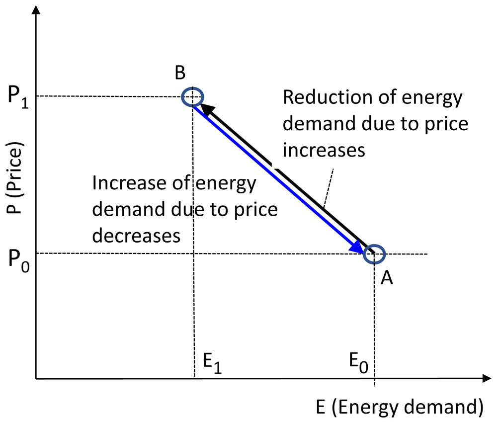
Figure 3a. Symmetric model specification.
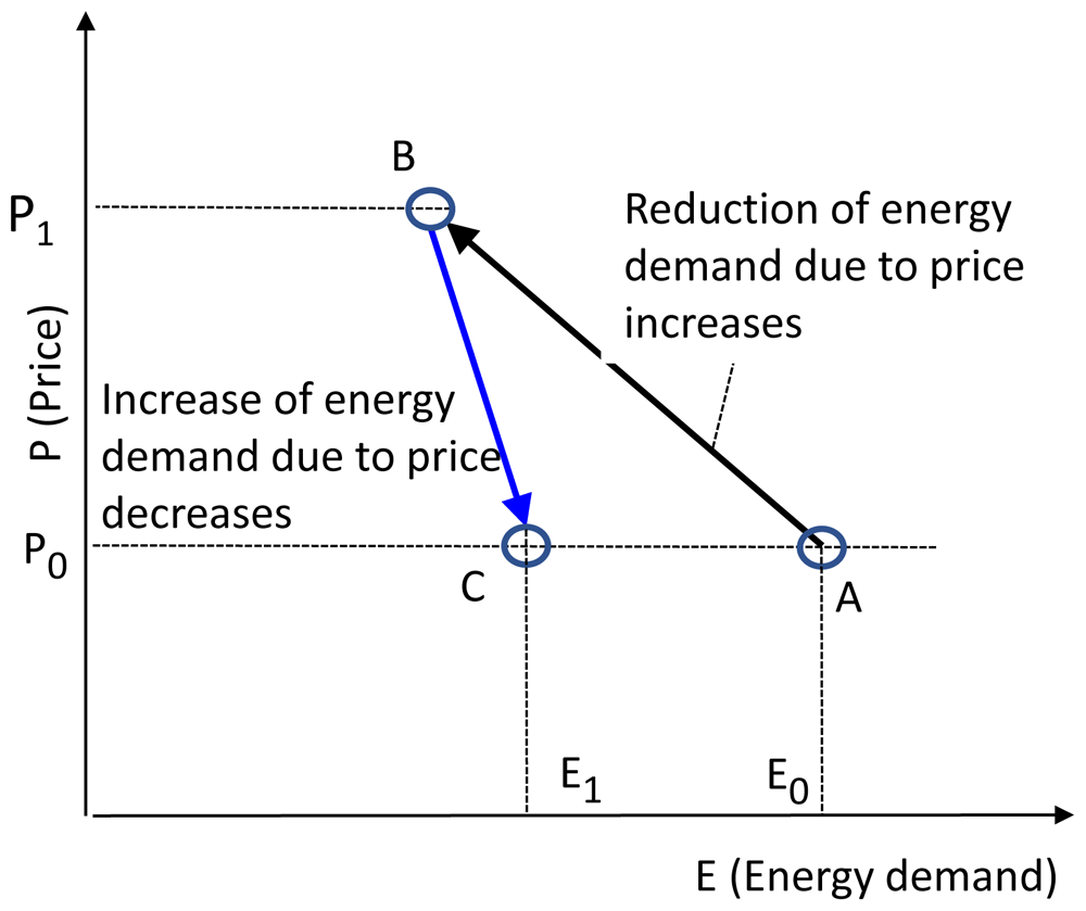
Figure 3b. Asymmetric model specification.
In the literature there are different asymmetric model specifications, taking into account differences for rising and falling prices as well as the historical maximum price, see e.g. 46. A dummy variable Dprise_t is used which is 1 if the fuel price is rising and 0 vice versa. The following basic equation is used and a simple OLS estimate is conducted:
with
α0 …… general long-term price elasticity
αrise … price elasticity for rising prices
and
Dprise_t = 1 if Pt > Pt-1
Dprise_t = 0 if Pt ≤ Pt-1
In this Equation (9), only the coefficient αrise is of interest and whether it is significantly different from zero or not. If it is, this proves that asymmetry exist.
The next issue of interest is the possible impact of historical maximum price. In some seminal contributions e.g. 10,11 introduced the possible role of a historical maximum price on energy demand, especially with respect to the oil price. Thereby, prices are decomposed into three components: (i) historical maximum price, (ii) price recoveries, and (iii) price cuts (see Figure 4). The idea is that in addition to asymmetries, having in mind the historical maximum price might influence consumers’ behaviour in a sustainable way.
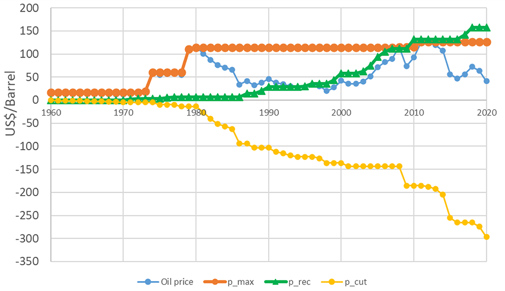
Figure 4. Principle of decomposition of the oil price in rising and falling prices as well as the historical maximum price.
Next, the price is decomposed as follows:
Note, that the specific elements of the data sources cited are based on the Equation (12) to Equation (15). The specific parameter used for the estimates presented in Figure 4 is the oil price p (Source: BP35), see also Table 5.
In an illustrative exercise with the oil demand data following Equation (9), (10) and (11) approaches, some new variables are defined:
Substitution of these definitions into Equation (1) to decompose the price results in Equation (15):
Estimating Equation (15) the only interest is in the price elasticities. Figure 6 quantitatively shows the exemplary estimates for pedagogic reasons for the three long-term price elasticities αmax, αrec and αcut over different periods of time. As seen in Figure 5, the trends are clearly towards declines of price and income elasticities over time. In addition, the estimates in Figure 5 depict that αmax and αrec has been quite significant. Only for αcut no reasonable estimates were obtained. And the figures for αmax and αrec are decreasing over time.
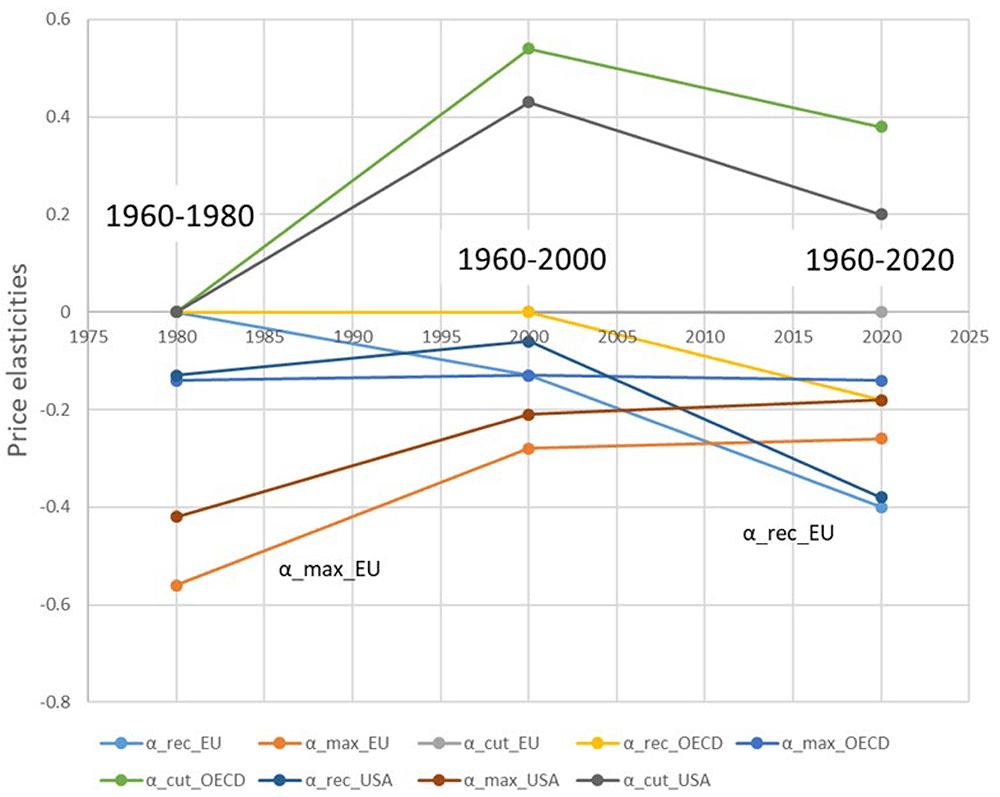
Figure 5. Estimates of the three components of price elasticities for EU-15, OECD and USA for long-term oil consumption over three periods applying the OLS approach (0 = value is not significant).
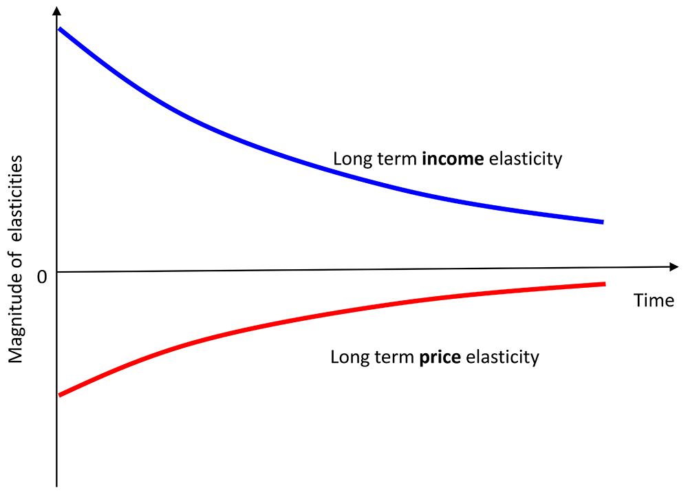
Figure 6. The principle of our idea of continuously decreasing absolute values of long-term income and price elasticities.
The results displayed in Figure 5 were obtained as follows: the year 1980 depicts the results for estimating the period 1960 to 1980, the values indicated in 2000 shows the results for estimating the period 1960 to 2000, and 2020 shows the values for the period 1960 to 2020. Note, that the specific elements of the data sources cited are based on the Equation (12) to Equation (15). The specific parameters used for the estimates presented in Figure 5 are
The detailed sources for these parameters are documented in Table 5.
The dynamics of elasticities
A very important reason for the investigation of the dynamics of elasticities is that price and income elasticities may not be constant over time, (see Figure 6). As mentioned earlier in this paper, in 1981 Kouris8 published the paper “Elasticities - Science or Fiction?” and argued that there are some severe problems with using constant elasticities. The major point of his criticism was that elasticities depend very strongly on the time periods they are estimated from.
So far it has been assumed that elasticities are constant. Haas et al.42 have shown an example for the gradually declining income elasticity in Austria’s electricity demand. Figure 7 qualitatively depicts the development of declining price and income elasticities as it has been increasingly observed over time.
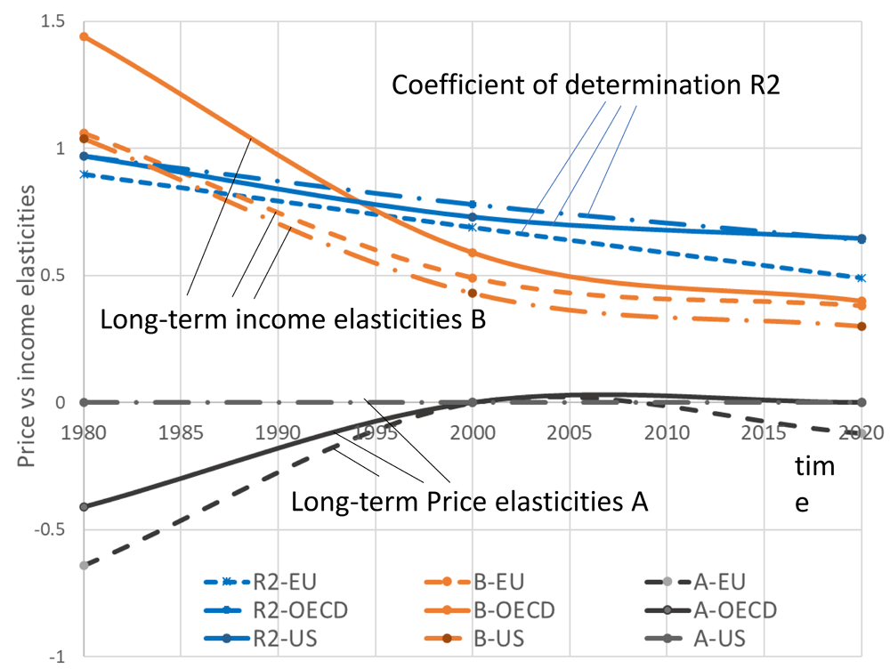
Figure 7. The dynamics of long-term price elasticities A and long-term income elasticities B as well as of R2 (coefficient of determination) for OECD, EU and USA.
Figure 7 quantitatively shows exemplary estimates for long-term price elasticities α and long-term income elasticities β over different periods of time. As can easily be seen, the trends are clearly towards declines of price and income elasticities over time. In addition, the corresponding statistical parameters for the coefficient of determination (R2) are documented in this figure and they are also declining, the longer the estimation period comes to recent years. This indicates that the coefficient of determination respectively the explanatory values of the economic parameters have decreased over time. The results displayed in Figure 7 were obtained as follows: the year 1980 shows the results for estimating the period 1960 to 1980, the values indicated in 2000 shows the results for estimating the period 1960 to 2000, and 2020 shows the values for the period 1960 to 2020.
Note, however, that for all estimates conducted in this work over different time periods the fittings of the coefficient of determination (R2) has been decreasing over time.
Structural breaks and disruptions
So far in this paper we have assumed continuous developments without any sudden changes. However, there is the question whether sudden specific events, e.g. oil price shocks, wars on oil, economic crisis like those in 2008/2009 or the current COVID19 crisis need a specific attention in modelling energy demand.
In this context, there are at least two approaches which are well known to model such kind of events: using Dummy variables and the Chow-Test.
Using Dummy variables
The first approach uses Dummy variables for the years where structural breaks are suspected, see Equation (16):
where:
Di ... Dummy variables (e.g., a specific year)
γ1, γ2, γ3, γ4 …Coefficients of the Dummy variables
with:
D1980= 1 if t ≤1980
D1988= 1 if t ≤1988
D1998= 1 if t ≤1998
D2011= 1 if t ≤ 2011
The logical reasoning and purpose of the dummies is to identify whether before and after the years indicated there is a significant difference. That is to say, in Equation (14) it is only of interest whether the coefficients γi are significantly different from zero or not. If they are, it proves that in these years structural breaks exist. The dummies are used for the following years and reasons: 1980 (first peak in oil prices), 1988 (first historical low in oil prices), 1998 (absolute historical low in oil prices), 2011 (last peak in world-wide oil prices).
The results of the example are documented in Table 4. As can be seen the results for the coefficients of the dummy variables indicate at a 90% level that there are several structural breaks in the investigated countries. For the EU-15 the years 1988 and 2011 indicate significant structural breaks, for the USA all years investigated show significant values for the dummies. For the OECD countries structural breaks were found for all investigated years except for 1980. Interestingly, the first year of a historical maximum in prices in 1980 shows a structural break in the USA only.
Table 4. Estimates of structural breaks in oil consumption using dummies for the years 1980 (first peak in oil prices), 1988 (first historical low in oil prices), 1998 (absolute historical low in oil prices) 2011 (last peak in oil prices), using OLS approach over the period 1960–2020.
| EU-15 | OECD | USA |
|---|
| D1980 | -0.06*) | -0.11*) | -0.23 |
| D1988 | -0.34 | -0.27 | -0.11 |
| D1998 | -0.05*) | -0.13 | -0.16 |
| D2011 | -0.19 | -0.23 | -0.22 |
Table 5. Databases used for analyses.
Note, that the specific elements of the data sources cited are based on the Equation (12) to Equation (16). The specific parameters used for the estimates presented in Table 4 are
Using the Chow Test
The Chow test, proposed by Gregory Chow in 1960, is usually an F-test of whether the true coefficients in two periods are equal. The principle is explained in Figure 8 where for two sub-periods of a longer one it is tested, whether the numbers for developments in energy demand E E0, E1 and E2 are the same.
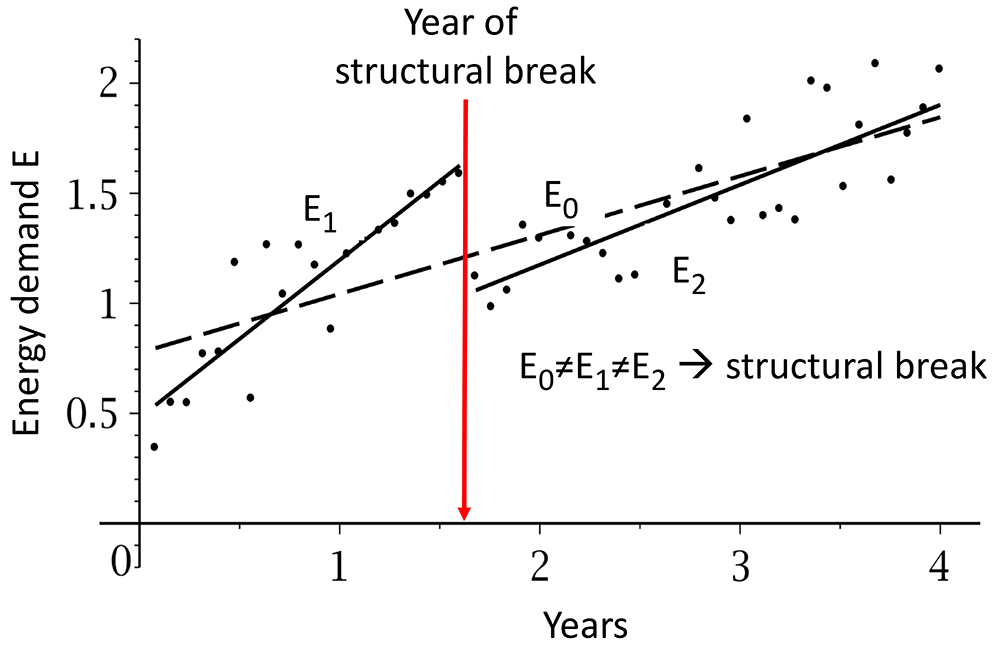
Figure 8. The Chow test for identifying structural breaks.
Such analyses were conducted for the years discussed above – 1980, 1988, 1998 and 2011 – using the Chow Test function in MICROFIT 5.5 and the result was simply that the presence of a structural break could not be rejected for any of these years or countries. Note, that the estimates were done for all years separately.
When wrapping up and taking into account both analysis methods discussed in this section (including the case studies calculated for the historical oil case), it is mainly to be expected that in a few years' time (when corresponding series of data are available) the analyses with these methods will also identify an effect of the COVID19 crisis for the years 2020/2021. Despite this, it is not expected to show a great difference in terms of patterns to those identified above for the case study of oil. Yet, the COVID19 crisis may give policymaking an additional boost (e.g. “EU Green Recovery Plan”), and perhaps motivate the implementation of intended structural changes and technology switches in the energy system much earlier than originally planned. Policy instruments play a core role in this context.
The effects of energy policy instruments
A major objective of this paper is to derive recommendations for energy policymakers from energy demand modelling lessons learned. Hanna and Gross25 conclude that policymakers could prepare more effectively for social, economic and political disruptions by integrating multi-disciplinary insights from a wide range of sciences and finally from repurposed energy systems optimization models. In Figure 2, the major policies available for interfering in energy demand and how they work have already been indicated. These are: subsidies, taxes, technical efficiency improvements such as standards, and – maybe most important of all – money spent for research and development. While the effect of subsidies is mainly to switch to and/or increase the share of energy use from low carbon technologies, the effect of taxes and technical efficiency improvements is more sophisticated.
The effects of energy policies have been analysed and discussed in several papers. The reduction of CO2 emissions of cars in the EU by analyzing the underlying mechanisms of standards, registration taxes and fuel taxes is discussed by Ajanovic et al.47. Regarding the impact of taxes, the seminal paper of Weitzman48 uses uncertainty to draw a wedge between price (i.e., a carbon tax) and quantity (i.e. emission permits) instruments that are equivalent in a deterministic and static setting. Suppliers (more precisely OPEC) and consumers (EU and other industrialized countries) use quantity instruments nowadays, although Wirl49 shows that the instrument prices dominates for both players (a supply monopoly and a consumer cartel). Karp et al.50 corroborate this finding numerically. The impact of energy policies on GHG emission reduction in passenger car mobility in the EU-15 is analysed in scenarios in Ajanovic51.
Regarding the reduction of energy demand the two major policy instruments are taxes and standards. The effect of the implementation of a tax is achieved from the price elasticity directly. If, for example. a price elasticity of -0.44 has been estimated (as in described in Ajanovic and Haas18 for road passenger transport) it is indicating that a 1% increase in price e.g. by a tax, it leads to a reduction of energy consumption of 0.44%.
Given this elasticity due to the analysis done in Ajanovic and Haas18 if a standard of 1% efficiency improvement would be introduced, a reduction of energy demand by only 0.56% (= 1 – 0.44 = 0.56) us the price elasticity) would be achieved. The delta to 1 is the rebound effect, for example an increase in service demand km driven due to the now cheaper service price for mobility because of the better efficiency, see also Andersen et al.52.
The conclusion for policy makers is twofold. On the one hand, due to the rather high rebound effect – see Ajanovic and Haas18 – of about 44% energy savings lost because of more km driven if fuel intensity is improved – technical standards with an effect of 56% as well as taxes with an effect of 44% as single separated policy instruments will have only limited success. On the other hand, however, if introduced in a combined leads to the effect that taxes compensate for the rebound due to standards and the full savings of 100% could ideally be achieved.
Conclusions
In this paper we have reviewed empirical energy demand models in the context of their historical development. The major conclusions of these analyses are ambiguous. On the one hand, econometric modelling of energy demand has made tremendous progress over the last about 30 years, especially regarding the mathematical tools but also with respect to specific approaches such as asymmetries, lags, and short-term vs long-term considerations. On the other hand, regarding further qualitative insights, the progress was very moderate especially with respect to dynamic adjustment mechanisms.
A major general conclusion regarding economic parameters is that their magnitude has been decreasing over time and hence the dynamics of elasticities is important. The smaller price elasticities are, the lower the impact of price changes. Consequently, the lower the impact of associated new/additional taxes on CO2-emissions, the higher the need for standards and technological innovations. Hence, the major useful policy suggestion based on this research is that energy efficiency is an important complementary measure to taxes.
A synthesis of the results of historical energy demand modelling shows that there is no need for "dramatizing" terminologies such as disruptions, shocks, or structural breaks to describe short-term, unexpectedly occurring exogenous influencing factors and/or events, but that these can be described in a pragmatic view in a longer-term context using already known and proven methods and models. This also includes observable discontinuities in energy demand development during the COVID19 pandemics, which in a few years will then most likely be described by the well-known influencing factors in modelling such as income, consumer spending or economic output (i.e., GDP), or short-term (voluntary or forced) behavioural changes associated with longer-term reversion to habitual patterns of energy consumption.
However, the momentum of the COVID19 pandemic can be used (and is being used, for example, in the “EU Green Deal” and “EU Green Recovery Plan”) to recognise and push for the importance of effective energy policy instruments and technological innovations. Against this background, perhaps some of the materials and methods presented in this paper are valuable for a better description of past, present and possible future energy demand developments during critical periods and its longer-term impacts. Optimistically, one may assume that the open science community will significantly contribute to further boosting energy demand modelling research in the future.
Ethics and consent
Ethical approval and consent were not required
Data availability statement
Underlying data
Table 5 shows the data used from the references documented:
Please note that no restrictions regarding the availability of data exist and that no automation tools or software codes were used in this process. Other researchers will be able to access the data in the same way as the authors and the authors do not have special access rights that others do not have.
Faculty Opinions recommendedReferences
- 1.
UNFCCC: Paris agreement. United Nations framework convention on climate change,
2015; 14.5.20. Reference Source
- 2.
Després J, Hadjsaid N, Criqui P, et al.:
Modelling the impacts of variable renewable sources on the power sector: reconsidering the typology of energy modelling tools.
Energy.
2015; 80: 486–495. Publisher Full Text
- 3.
Prataviera E, Romano P, Carnieletto L, et al.:
EUReCA: an open-source Urban Building Energy Modeling tool for the efficient evaluation of cities energy demand.
Renew Energy.
2021; 173: 544–560. Publisher Full Text
- 4.
Pindyck RS, Rubinfeld DL:
Econometric models & Economic Forecasts. McGraw-Hill, 3rd Ed, 1991.
- 5.
Ryan DL, Plourde A:
Empirical Modelling of energy demand. In: Joanne Evans, Lester Hunt: International handbook on the economics of energy. Edward Elgar Publishing, 2009; 112–143. Reference Source
- 6.
Meadows DH, Meadows DL, Randers J, et al.:
The Limits of Growth. Publisher Potomac Associates - Universe Books,
1972. Reference Source
- 7.
Pindyck RS:
The Structure of world energy demand. MIT press, 1979. Reference Source
- 8.
Kouris G:
Elasticities - science or fiction?
Energy Econ.
1981; 3(2): 66–70. Publisher Full Text
- 9.
Madlener R:
Econometric Analysis of Residential Energy Demand: A survey.
The Journal of Energy Literature.
1996; II(2): 3–32.
- 10.
Gately D:
Imperfect Price-Reversibility of U.S. Gasoline Demand: Asymmetric Responses to Price Increases and Declines.
The Energy Journal.
1992; 13(4): 179–207. Reference Source
- 11.
Gately D:
The Imperfect Price-Reversibility of World Oil Demand.
The Energy Journal.
1993; 14(4): 163–182. Reference Source
- 12.
Dargay JM:
The irreversible Effects of High Oil Prices: Empirical Evidence for the Demand for Motor Fuels in France, Germany and the UK. In: Energy Demand: Evidence and Expectations. Surrey University Press, 1992. Reference Source
- 13.
Walker IO, Wirl F:
Irreversible Price-Induced Efficiency Improvements.
The Energy Journal.
1993; 14(4): 183–205. Publisher Full Text
- 14.
Gallo A, Paul Mason P, Shapiro S, et al.:
What is behind the increase in oil prices? Analyzing oil consumption and supply relationship with oil price.
Energy.
2010; 35(10): 4126–4141. Publisher Full Text
- 15.
Haas R, Schipper L:
Residential energy demand in OECD-countries and the role of irreversible efficiency improvements. Evidence from the period 1970-1993.
Energy Econ.
1998; 20(4): 421–442. Publisher Full Text
- 16.
Engsted T, Bentzen J:
Expectations, adjustment costs, and energy demand.
Resource and Energy Economics.
1993; 15: 371–385. Reference Source
- 17.
Ajanovic A, Dahl C, Schipper L:
Modelling transport (energy) demand and policies — An introduction.
Energy Policy.
2012; 41: iii–xiv. Publisher Full Text
- 18.
Ajanovic A, Haas R:
The role of efficiency improvements vs. price effects for modeling passenger car transport demand and energy demand—Lessons from European countries.
Energy Policy.
2012; 41: 36–46. Publisher Full Text
- 19.
Dunstan RH, Schmidt RH:
Structural changes in residential energy demand.
Energy Econ.
1988; 10(3): 206–212. Publisher Full Text
- 20.
Fouquet R:
The impact of VAT introduction on UK residential energy demand: An investigation using the cointegration approach.
Energy Econ.
1995; 17(3): 237–247. Publisher Full Text
- 21.
Shahbaz M, Naceur K, Mantu KM, et al.:
Are fluctuations in natural gas consumption per capita transitory? Evidence from time series and panel unit root tests.
Energy.
2014; 78: 183–195. Publisher Full Text
- 22.
Chiu FP, Hsu CS, Ho A, et al.:
Modeling the price relationships between crude oil, energy crops and Biofuels.
Energy.
2016; 109: 845–857. Publisher Full Text
- 23.
Kemfert C, Lorenz C, Traber T, et al.:
Energy Efficiency: A Key Challenge of the Energiewende. In: Energiewende "Made in Germany": Low Carbon Electricity Sector Reform in the European Context. 2018; 173–191. Publisher Full Text
- 24.
Kemfert C:
Estimated substitution elasticities of a nested CES production function approach for Germany.
Energy Econ.
2020; 20(3): 249–264.
- 25.
Hanna R, Gross R:
How do energy systems model and scenario studies explicitly represent socio-economic, political and technological disruption and discontinuity? Implications for policy and practitioners.
Energy Policy.
2021; 149: 111984. Publisher Full Text
- 26.
Burt G:
Why are we surprised at surprises? Integrating disruption theory and system analysis with the scenario methodology to help identify disruptions and discontinuities.
Technol Forecast Soc Change.
2007; 74(6): 731–749. Publisher Full Text
- 27.
Ayres RU:
On forecasting discontinuities.
Technol Forecast Soc Change.
2000; 65(1): 81–97. Publisher Full Text
- 28.
Densing M, Panos E, Hirschberg S:
Meta-analysis of energy scenario studies: example of electricity scenarios for Switzerland.
Energy.
2016; 109: 998–1015. Publisher Full Text
- 29.
Krarti M, Aldubyan M:
Review analysis of COVID-19 impact on electricity demand for residential buildings.
Renew Sustain Energy Rev.
2021; 143: 110888. PubMed Abstract
| Publisher Full Text
| Free Full Text
- 30.
Navon A, Machlev R, Carmon D, et al.:
Effects of the COVID-19 Pandemic on Energy Systems and Electric Power Grids—A Review of the Challenges Ahead.
Energies.
2021; 14(4): 1056. Publisher Full Text
- 31.
Malliet P, Reynès F, Landa G:
Assessing Short-Term and Long-Term Economic and Environmental Effects of the COVID-19 Crisis in France.
Environ Resour Econ (Dordr).
2020; 76(4): 867–883. PubMed Abstract
| Publisher Full Text
| Free Full Text
- 32.
Ansari D, Kemfert C:
A Nomadic Journey - Simulating the Effect of COVID-19 and Production Shifts on Crude Oil Prices.
Reference Source
- 33.
Jiang P, Van Fan Y, Klemes JJ:
Impacts of COVID-19 on energy demand and consumption: Challenges, lessons and emerging opportunities.
Appl Energy.
2021; 285: 116441. PubMed Abstract
| Publisher Full Text
| Free Full Text
- 34.
Cheshmehzangi A:
COVID-19 and household energy implications: what are the main impacts on energy use?
Heliyon.
2020; 6(10): e05202. PubMed Abstract
| Publisher Full Text
| Free Full Text
- 35.
BP:
Statistical review. 2022. https://www.bp.com/content/dam/bp/business-sites/en/global/corporate/xlsx/energy-economics/statistical-review/bp-stats-review-2021-all-data.xlsx
- 36.
OPEC Annual Statistical Bulletin. 57th Edition, Table 4.7.
2022. https://asb.opec.org/data/ASB_Data.php
- 37.
OECD: Dataset: Consumer price indices (CPIs) - Complete database. https://stats.oecd.org/index.aspx?DataSetCode=PRICES_CPI
- 38.
World bank. https://data.worldbank.org/indicator/NY.GDP.MKTP.CD
- 39.
Pesaran MH:
Time Series and Panel Data Econometrics. Oxford University Press, Oxford, 2015. Reference Source
- 40.
Lee CC, Chiu YB:
Modeling OECD energy demand: An international panel smooth transition error-correction model.
International Review of Economics and Finance.
2013; 25: 372–383. Publisher Full Text
- 41.
Bahram P, Hashem PM:
Time Series Econometrics using Microfit 5.0: A User's Manual. Oxford University Press, Oxford, 2019.
- 42.
Haas R, Biermayr P, Zöchling J, et al.:
Impacts on electricity consumption of household appliances in Austria: a comparison of time series and cross-section analyses.
Energy Policy.
1998; 26(13): 1031–1040. Publisher Full Text
- 43.
Farhani S, Solarin SA:
Financial development and energy demand in the United States: New evidence from combined cointegration and asymmetric causality tests.
Energy.
2017; 134: 1029–1037. Publisher Full Text
- 44.
Kirchgässner G, Kübler K:
Symmetric or asymmetric price adjustments in the oil market: An empirical analysis of the relations between international and domestic prices in the Federal Republic of Germany, 1972–1989.
Energy Econ.
1992; 14(3): 171–185. Publisher Full Text
- 45.
Haas R, Zöchling J, Schipper L:
The relevance of irreversibility issues for Residential oil and natural gas demand - Evidence from selected OECD countries 1970 - 1995.
OPEC-Review.
1998; XXII(2): 113–145.
- 46.
Gately D, Huntington HG:
The Asymmetric Effects of Changes in Price and Income on Energy and Oil Demand.
The Energy Journal.
2001; 23(1).
- 47.
Ajanovic A, Haas R:
The impact of energy policies in scenarios on GHG emission reduction in passenger car mobility in the EU-15.
Renew Sustain Energy Rev.
2017; 68(2): 1088–1096. Publisher Full Text
- 48.
Weitzman ML:
Prices vs. Quantities.
Rev Econ Stud.
1974; 41(4): 477–491. Publisher Full Text
- 49.
Wirl F:
Global Warming: Prices versus Quantities from a Strategic Point of View.
J Environ Econ Manage.
2012; 64(2): 217–229. Publisher Full Text
- 50.
Karp L, Siddiqui S, Strand J:
Dynamic Climate Policy with Both Strategic and Non-strategic Agents: Taxes Versus Quantities.
Environmental & Resource Economics.
2016; 65(1): 135–158.
- 51.
Ajanovic A, Haas R, Wirl F:
Reducing CO2 emissions of cars in the EU: analyzing the underlying mechanisms of standards, registration taxes and fuel taxes.
Energy Efficiency.
2016; 9: 925–937. Publisher Full Text
- 52.
Andersen KS, Termansen LB, Gargiulo M, et al.:
Bridging the gap using energy services: demonstrating a novel framework for soft linking top-down and bottom-up models.
Energy.
2019; 169: 277–293. Publisher Full Text