Coexistence of chaotic attractor and unstable limit cycles in a 3D dynamical system

Dana Constantinescu; Gheorghe Tigan; Xiang Zhang

doi:10.12688/openreseurope.13590.1

Coexistence of chaotic attractor and unstable limit cycles in a 3D dynamical system

Dana Constantinescu
,
Gheorghe Tigan ,
Xiang Zhang

Article

Authors & roles Authors

Peer review record Peer review

Metrics

Cite

Section

Research Article

Published

May 17, 2021

DOI

https://doi.org/10.12688/openreseurope.13590.1

Versions

May 17, 2021 (Version of Record 1.0)

European Commission

Grant ID(s): 777911
National Office of Philosophy and Social Sciences

Grant ID(s): 11871334

Views

101

Downloads

Citations

See full metrics

chaotic attractors, bifurcation, limit cycle, algebraic invariant surfaces, global dynamics

Abstract

The coexistence of stable limit cycles and chaotic attractors has already been observed in some 3D dynamical systems. In this paper we show, using the T-system, that unstable limit cycles and chaotic attractors can also coexist. Moreover, by completing the characterization of the existence of invariant algebraic surfaces and their associated global dynamics, we give a better understanding on the disappearance of the strange attractor and the limit cycles of the studied system.

Corresponding author

Gheorghe Tigan

0000-0001-7083-4666

gheorghe.tigan@upt.ro

Grant information

This project has received funding from the European Union’s Horizon 2020 research and innovation programme under the Marie Skłodowska-Curie grant agreement No [777911], (project Dynamics). XZ is partially supported by the National Social Science Fund of China, grant number 11871334.

The funders had no role in study design, data collection and analysis, decision to publish, or preparation of the manuscript.

This work is licensed under a Creative Commons Attribution 4.0 International License.

First version published

May 17, 2021 (https://doi.org/10.12688/openreseurope.13590.1)

Latest version published

May 17, 2021 (https://doi.org/10.12688/openreseurope.13590.1)

Introduction

The Lorenz system is considered a benchmark for systems with complex (chaotic) dynamics. It was one of the first examples of 3D autonomous differential systems showing the existence of a strange attractor. The contrast between the simplicity of its equations and the complexity of its dynamical behavior attracted a lot of attention since its publication in 1963, but its thorough study was possible only when computational devices were developed enough to support long and laborious numerical simulations.

Many other systems with chaotic behavior and simple analytical form were obtained later, such as: the Rössler system¹ in 1979, Chua model² in 1986, and a list of about 18 systems not previously known provided by Sprott³ in 1994. For these systems and others, not only chaotic behaviors but also other dynamics, e.g. integrability and global dynamics, were studied. See for instance^4–8.

However, interest in the Lorenz system has not diminished. In 1999, Chen and Ueta proposed a dual system with a chaotic attractor that is not equivalent to the Lorenz attractor⁹ and in 2002, Lü and Chen proposed a new chaotic system¹⁰. A more general Lorenz-type system was defined in 2006¹¹ and many studies are related to common properties of the systems in this family.

In a class of systems, not only general but also particular properties are important. Some specific systems in the Lorenz family have specific properties and/or applications and deserve to be separately studied. This is the case for the T-system introduced in 2008 in 12. This is a 3D autonomous quadratic polynomial system with three real parameters a, b, c, given by

\dot{x} = a (y - x), \dot{y} = (c - a) x - a x z, \dot{z} = - b z + x y . (1)

Properties and potential applications of system (1) have been reported in recent years in many papers. For example, the existence of heteroclinic orbits in the T-system connecting equilibrium points was studied using Lyapunov functions in 13 or the Shilnikov method in 14. The Hopf bifurcations¹⁵ and bifurcations with delayed feedback¹⁶ in the T-system were studied using analytical methods and a classification of chaotic regimes using competitive modes was realized in 17. Some methods for the control of its chaotic dynamics and synchronization were proposed in 18–20. General techniques for finite-time stabilization of 3D chaotic systems were exemplified using the T-system²¹. A fractional-order T-system was derived and studied in 22. It was shown that system (1) has potential applications in secure communications^23–25. These prove the interest in the study of system (1).

The aim of the present work is to prove the coexistence of a chaotic attractor together with two isolated unstable periodic orbits in the T-system (1), to describe properties of global dynamics in the cases when it has algebraic invariant surfaces, and to correlate these results with other information obtained using different dynamical methods.

We note that for the coexistence of limit cycles and chaotic attractor, Sprott, Wang and Chen²⁶ provided (perhaps) the first example, namely

\dot{x} = y z + a, \dot{y} = x^{2} - y, \dot{z} = 1 - 4 x,

showing the coexistence of a point attractor, a chaotic attractor and a stable limit cycle when the parameter a was chosen suitably. Li and Sprott²⁷ constructed an example given by

\dot{x} = y + y z, \dot{y} = - x z + y z, \dot{z} = - a x - x y + b,

which has five coexisting attractors: a limit cycle, two equilibria and two strange attractors in different attractor basins for suitably chosen values of the parameters.

We remark that the periodic orbit in 26,27 is an attractor (a stable limit cycle). In this work, the twin isolated periodic orbits we obtain are unstable and have a one dimensional unstable invariant manifold and a one dimensional stable invariant manifold. Later on, we will show that the T-system is a special case of the generalized Lorenz system, which had not exhibited the coexistence of a chaotic attractor with isolated periodic orbits in previous studies.

The paper is structured as follows: Bifurcations, chaos, unstable periodic orbits is devoted to the study of the bifurcations of T-systems and contains our new discovery, i.e. the coexistence of a chaotic attractor with isolated unstable periodic orbits; in First integrals and invariant algebraic surfaces the T-systems are identified as having algebraic invariant surfaces; and their global dynamics are analysed in Global dynamics of the T-system with invariant algebraic surfaces. Finally, conclusions and discussions are presented.

Bifurcations, chaos, unstable periodic orbits

If a = 0 system (1) is linear, it has minor interest. In what follows we will focus on the case a > 0 (the case a < 0 can be treated similarly).

Using the transformation of variables

\tilde{x} = \frac{x}{\sqrt{a}}, \tilde{y} = \frac{y}{\sqrt{a}}, \tilde{z} = z, τ = a t, (2)

and the transformation of parameters (a, b, c) ↦ (a, m, n) given by $m = \frac{c}{a} - 1$ and $n = \frac{b}{a}$ , where a > 0, system (1) is topologically equivalent to

\dot{x} = y - x, \dot{y} = m x - x z, \dot{z} = - n z + x y, (3)

where "~" was neglected for the sake of simplicity. We notice that the transformation of parameters is invertible. System (3) has the advantage of having only two parameters.

Equilibria and their stability

A stable focus in a 3D system is an equilibrium that has a negative eigenvalue and two complex conjugate eigenvalues with negative real parts, while a saddle focus is an equilibrium that has a negative (or positive) eigenvalue and two complex conjugate eigenvalues with positive (respectively negative) real parts.

Theorem 1. For m > 0 and n > 0, system (3) has three equilibria:

O = (0, 0, 0) and P_{\pm} = (\pm \sqrt{m n}, \pm \sqrt{m n}, m) .

Moreover, the following statements hold.

(a) The equilibrium point O is a saddle with dim (W^u (O)) = 1 and dim (W^s (O)) = 2. The equilibria P_± are stable foci if m(n – 1) + n + 1 > 0, or saddle foci with dim (W^u (P_±)) = 2 and dim (W^s (P_±)) = 1 if m(n – 1) + n + 1 < 0.
(b) If $m = m_{H} := \frac{1 + n}{1 - n}$ and 0 < n < 1, system (3) undergoes a nondegenerate Hopf bifurcation at P_±. Moreover, the equilibria P_± are both unstable weak foci on the two dimensional center manifold, and for 0 < m_H – m ≪ 1 from each of P_± bifurcates a limit cycle which has a one dimensional unstable manifold and a one dimensional stable manifold.

Proof: the existence of equilibria follow from easy calculations.

a). The properties on O follows from the observation that the characteristic polynomial of system (3) at O, i.e.

f_{O} (λ) = (λ + n) (λ^{2} + λ - m),

has one positive and two negative roots.

The properties of P_± follow from their characteristic polynomials

f_{P_{\pm}} (λ) = λ^{3} + (n + 1) λ^{2} + (m n + n) λ + 2 m n, (4)

which has a negative root λ₁ < 0 and two complex conjugated roots λ_2,3 = α ± iβ. Here we have used the fact that the equation

x^{3} - p x^{2} - q x - r = 0 with r < 0 and p < 0,

has three roots with negative real parts if and only if r + pq > 0, or one negative real root and two roots with positive real parts if and only if r + pq < 0, respectively.

The real part of λ_2,3 is negative if and only if –2mn + (–n –1) (–mn – n) > 0. Because n > 0 this condition reads m(n – 1) + n + 1 > 0.

The real part of λ_2,3 is positive if and only if –2mn + (–n – 1) (–mn – n) < 0, so P_± are saddle foci with dim (W^u (P_±)) = 2 and dim (W^s (P_±)) = 1. This proves statement (a).

(b). According to the proof of (a), we treat the eigenvalues of system (3) at P_± as a function of m, and take

λ_{2, 3} (m) = α (m) \pm i ω (m) .

Standard computations show that α (m) = 0 if and only if $m = m_{H} := \frac{1 + n}{1 - n}$ > 0. In this case $ω = \sqrt{\frac{2 n}{1 - n}} > 0$ .

Differentiating the relation f_{P_±} (λ(m)) = 0 with respect to m, we obtain

{\frac{d α (m)}{d m} |}_{m = m_{H}} = \frac{1}{2} \frac{{(1 - n)}^{2} n}{(3 - n) n + 1 - n^{3}} > 0 .

The first Lyapunov coeffcient²⁸ is

l_{1} (m_{H}) = \frac{ω (3 + ω^{2}) (6 + 4 ω^{2} + 2 ω^{4} + ω^{6})}{2 (1 + ω^{2}) (1 + 6 ω^{2} + 5 ω^{4} + ω^{6}) (4 + 12 ω^{2} + 8 ω^{4} + ω^{6})} .

Notice that it is always positive, l₁ (m_H) > 0.

The above calculations show that when m = m_H, system (3) restricted to the two dimensional center manifold at P₊ always has the equilibrium P₊ as an unstable weak focus. By symmetry, when m = m_H system (3) restricted to the two dimensional center manifold at P_– always has the equilibrium P_– as an unstable weak focus. Combining the analyses of the equilibria P_± when m ≠ m_H, we get that, for $0 < \frac{1 + n}{1 - n} - m ≪ 1,$ system (3) has a limit cycle bifurcating from each of P_±. Whereas if we use notations from the Stable Manifold Theorem for periodic orbits (29, page 225), each of the limit cycles has a two dimensional unstable manifold and a two dimensional stable manifold, which both contain the limit cycle as a one dimensional submanifold and transversally intersect on it. One may conclude that each of the two limit cycles has a one dimensional unstable manifold and a one dimensional stable manifold. This proves the theorem.

Dynamical zones in the parametric plane

The regions of the plane (n, m) where system (3) has different dynamical properties are presented in Figure 2, in which the Hopf bifurcation curve (h) given by

m = \frac{1 + n}{1 - n} with 0 < n < 1,

splits the plane (n, m) into two zones: R₃ and R₁ ∪ R₂.

In the region R₃ with $m > \frac{n + 1}{1 - n}$ , the equilibria P_± are saddle foci with a one dimensional stable manifold and a two dimensional unstable manifold. The local properties of these equilibria foresee the possibility of existence of the chaotic attractor. Using m = 2 and $n = \frac{m - 1}{m + 1} + K = \frac{1}{3} + K$ for K = –0.3, –0.2, –0.1, respectively, and taking the initial values $x (0) = \sqrt{m (m - 1) / (m + 1)} + 0.101,$ $y (0) = \sqrt{m (m - 1) / (m + 1)} - 0.201$ and z(0) = m + 0.302, we get the three figures showing the positive orbits of the initial value problem, see Figure 1. Note that the initial point of the orbit has a relatively fixed position compared with P₊, and that the positive limit of the orbit becomes much more chaotic when n increases from 0 to near the Hopf bifurcation value.

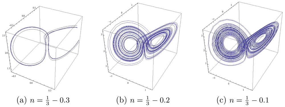
Figure 1. A positive orbit before Hopf bifurcation for m = 2 shows the butterfly attractor.

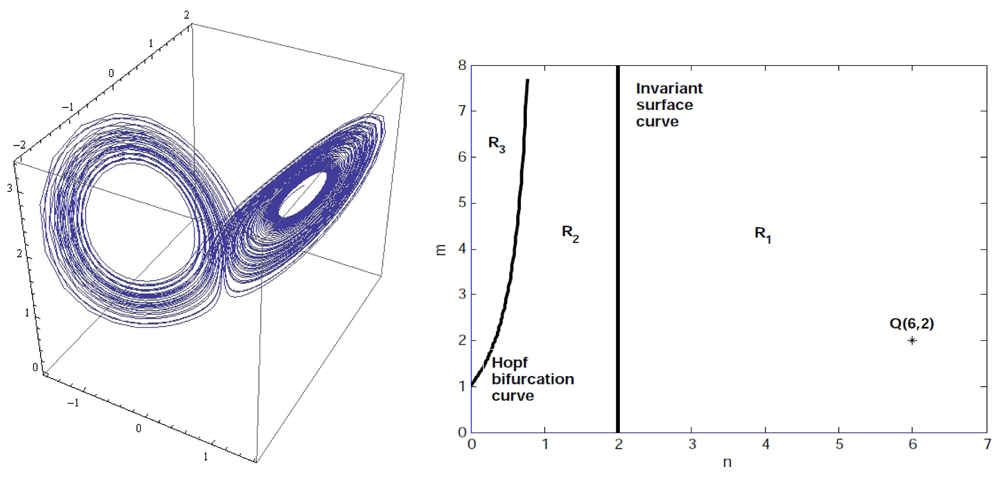
Figure 2. A butterfly attractor exists at the Hopf bifurcation value m = 2 and $n = \frac{1}{3}$ (left).

Regions with different dynamical properties in the (m, n) plane (right).

At the Hopf bifurcation values $n = \frac{m - 1}{m + 1}$ for m > 1, the local structures of the equilibria are similar to the ones for m > 1 and $0 < n < \frac{m - 1}{m + 1}$ but now the P_± are unstable weak foci of order 1 on their center manifolds, respectively, which also forces the existence of chaotic attractor. Figure 2 illustrates such a butterfly attractor for system (3) with m = 2; where the orbit starts at $x (0) = \sqrt{m (m - 1) / (m + 1)} + 0.101,$ $y (0) = \sqrt{m (m - 1) / (m + 1)} - 0.201$ , z(0) = m + 0.302.

When n increases from (m – 1)/(m + 1) but is less than 2, the parameters are in the region R₂. System (3) has the equilibria P_± as stable foci on the two dimensional stable manifolds $M_{\pm}^{s}$ approaching, respectively, the center manifolds $M_{\pm}^{c}$ of system (3) at P_± when n = (m – 1)/(m + 1). Then there is a limit cycle bifurcating from each of P_± on $M_{\pm}^{s}$ , respectively. By the continuity of orbits with respect to parameters we have shown that for 0 < n – (m – 1)/(m + 1) ≪ 1 system (3) has also a butterfly attractor and two additional isolated periodic orbits with a one dimensional unstable manifold and a one dimensional stable manifold. Figure 3 illustrates the stable focus, the periodic orbit and the butterfly attractor of system (3) when m = 2 and $n = \frac{1}{3}$ + 0.01, where the initial values of the three orbits have the same x and y coordinates, x(0) = y(0) = 5.001, but different z coordinates, which are z(0) = –2.515 in(a), –1.424 in (b) and –0.515 in (c), respectively.

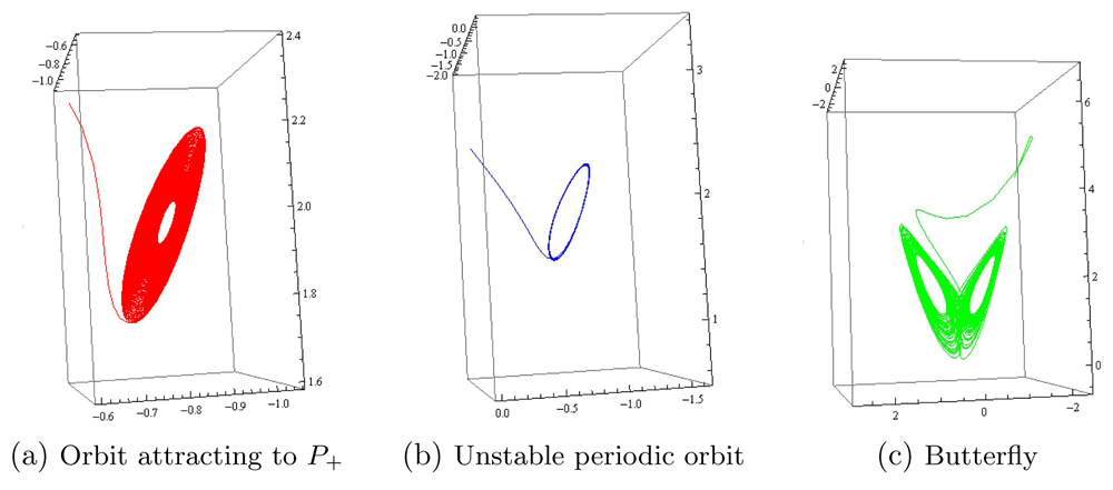
Figure 3. Three orbits of system (3) when m = 2 and n = 1/3 + 0.01, which is after Hopf bifurcation.

Now for system (3) with m = 2 and $n = \frac{1}{3}$ + 0.01, we take another three initial points, whose x and y coordinates are the same with x(0) = y(0) = –5.001, and z coordinates are the same as the previous three, i.e. z(0) = –2.515, –1.424 and –0.515, respectively. Putting all these six orbits in a unique picture, one gets the figure given in Figure 4, which contains two stable foci, two isolated unstable periodic orbits with, respectively, a one dimensional stable invariant manifold and a butterfly attractor.

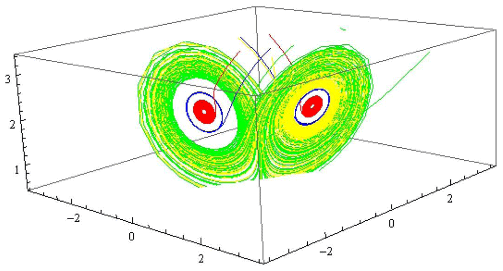
Figure 4. The six positive orbits of system (3) when m = 2, $n = \frac{1}{3}$ + 0:01: the red ones have limits at P_±, respectively, the blue ones have their limits as one of the two unstable limit cycles on the two dimensional invariant manifolds, and the green and yellow ones approach the butterfly attractor.

In order to get more evidence on the existence of a strange attractor at the Hopf bifurcation values, or after and before these values, we computed the Lyapunov exponents using the method presented in 30 for values of m ∈ [1, 4].

By our calculation at the Hopf bifurcation values, it was observed that the first Lyapunov exponent is positive for all values of m > 1. Moreover, the first Lyapunov exponent increases when the values of m increase. The second Lyapunov exponent is null and the third one is negative, which shows that the butterfly attractor strange and the dynamics of the system in the basin of attraction of this attractor are chaotic³⁰. Figure 5 presents the values of Lyapunov exponents, which were computed for various values of m; using a long orbit of (x(0), y(0), z(0)) = (5.001, 5.001, –2.515).

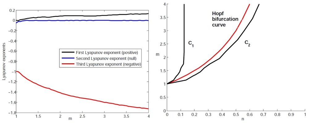
Figure 5. The Lyapunov exponents at the Hopf bifurcation values for m ∈ [1, 4] (left).

The zone situated between C₁ and C₂ is formed by couples (n, m) for which the corresponding system has a strange attractor (right).

We note that the existence of a strange attractor before and after the Hopf bifurcation can be also proved through the computation of the Lyapunov exponents for systems whose parameters (n, m) are situated near the Hopf bifurcation curve. In Figure 5, the zone situated between the curves C₁ and C₂ is formed by parameters (n, m) for which the dynamical system has a positive, a null and a negative Lyapunov exponent, i.e. there is a strange attractor coexisting with two saddle foci P_± in the region R₃ (i.e. $m > \frac{1 + n}{1 - n} > 0$ ) or with the two stable equilibria P_± and the unstable limit cycles in R₂ (i.e. $0 < \frac{1 + n}{1 - n} - m < ρ,$ with ρ a suitable positive small number).

First integrals and invariant algebraic surfaces

The purpose of many studies is to understand the global dynamics of systems from the Lorenz family. A first step for this is to study subclasses of these systems, for example, the subclass of systems with invariant algebraic surfaces. Such surfaces in the Lorenz system were studied in 31. Darboux polynomials in Chen and Lü systems were studied in 32–34 and a generalization is achieved in 35. The non-algebraic integrability of the Chen and Lü systems was studied in 36 and 37, respectively.

The global dynamics of the Lorenz system with invariant algebraic surfaces was studied in 38 and similar studies for the Chen system were performed in 32. The description of the dynamics in generalized Lorenz systems with invariant algebraic surfaces was performed in 39. In this work, our study on the existence of invariant algebraic surfaces of the T-system and its related global dynamics will be helpful to understand the disappearance of the chaotic attractor.

Invariant surfaces and first integrals are important tools for understanding the behavior of dynamical systems. A Darboux polynomial of the 3D polynomial differential system

\dot{x} = P (x, y, z), \dot{y} = Q (x, y, z), \dot{z} = R (x, y, z), (5)

with P, Q, R ∈ ℝ[x, y, z] as the ring of polynomials, is a polynomial F ∈ ℂ[x, y, z] which fulfills

\frac{\partial F}{\partial x} P + \frac{\partial F}{\partial y} Q + \frac{\partial F}{\partial z} R = k F,

for some polynomial k ∈ ℂ[x, y, z], which is called the cofactor³⁵.

If k ≠ 0, then F = F(x, y, z) is called a proper Darboux polynomial. If k = 0, then F = F (x, y, z) is a first integral of (5), that is $\frac{d F}{d t} |$ ₍₅₎ = 0. If system (5) has two functionally independent first integrals F₁ (x, y, z) and F₂ (x, y, z) defined in a domain Ω ⊂ ℝ³, then the orbits of the system in Ω are contained in the curves {F₁ (x, y, z) = h₁} ∩ {F₂ (x, y, z) = h₂} for some h₁, h₂ ∈ ℝ, and the system is completely integrable.

If F (x, y, z) is a Darboux polynomial of (5), then the set

S_{F} = {(x, y, z) \in ℝ^{3} | F (x, y, z) = 0}

is invariant under the flow of the system (5). It justifies its name invariant algebraic surface.

A generalized Lorenz system given by

\dot{x} = A (y - x), \dot{y} = B x + C y - x z, \dot{z} = D z + x y, (6)

was studied in 35, where the existence of invariant algebraic surfaces have been obtained. It has been shown in Theorem 1.1 from 35 that there are only six cases in which system (6) has Darboux polynomials, namely: a) D = −2A, when the cofactor is k = −2A, b) D = C and B = 0, when the cofactor is k = 2C, c) A = −C and D = C, when the cofactor is k = 2C, d) A = −C/3 and D = 0, when the cofactor is k = 4C/3, e) A = −C and D = 4C, when the cofactor is k = 4C, f) B = 2A + C and D = −6A − 2C, when the cofactor is k = −4A. In 40 the authors found the seventh case, C = D = 0, when system (6) has the first integral F(x , y, z) = y² + z² − 2Bz. The global dynamics in each case were described in 40 and 39. We will apply the results of these papers to study system (3).

Theorem 2. System (3) with a > 0 has algebraic invariant surfaces if and only if

(a) either n = 2, when the algebraic invariant surface is x² − 2z = 0,
(b) or m = 2, n = 6 when the algebraic invariant surface is
$x^{4} - 4 x^{2} z - 4 y^{2} + 16 x y - 16 x^{2} = 0,$
(c) or n = 0, when there are infinitely many algebraic invariant surfaces with the equation
$y^{2} + z^{2} - 2 m z = c s t .$

Proof: The proof is a consequence of Theorem 1.1 in 35, which shows that system (6) admits proper Darboux polynomials only in two cases, namely D = –2A (when the Darboux polynomial is ${\bar{F}}_{1}$ (x, y, z) = x² – 2Az), and B = 2A and D = –6A (when the Darboux polynomial is ${\bar{F}}_{2}$ (x, y, z) = x⁴ – 4Ax²z – 4A²y² + 16A²xy – 16A²x²). These conditions read n = 2, m = 2 and n = 6 in system, respectively (3). The corresponding invariant surfaces, obtained from the Darboux polynomials through the transformation (2) are x² – 2z = 0 and x⁴ – 4x²z – 4y² + 16xy – 16x² = 0, respectively.

In the case n = 0, we have C = D = 0 so the polynomial

\bar{F} (x, y, z) = y^{2} + y^{2} - 2 m z

is a first integral of system (6). From (2) it results that F (x, y, z) = y² + z² – 2mz is a first integral of (3). In this case we have infinitely many invariant surfaces with the equation F (x, y, z) = cst. Consequently, ℝ³ is practically foliated by the invariant cylinders y² + (z – m)² = r² for 0 < r ∈ ℝ.

Global dynamics of the T-system with invariant algebraic surfaces

In the following we will denote the orbit of system (3) passing q₀ ∈ ℝ³ by O (q₀) = {φ_t (q₀) | t ∈ ℝ} and by α (q₀) (ω (q₀)), the α (ω) limit sets of O (q₀).

Theorem 2 in 39 shows that, for a ≠ 0, all orbits of the generalized Lorenz system (6) starting from outside the algebraic invariant surface S_F are heteroclinic: they either all positively approach the surface and negatively go to infinity (i.e. ω (q₀) ⊂ S_F and α (q₀) = ∞), or converse.

We now present the global dynamics of the T-systems, and its sketch proof for completeness. Set

\begin{array}{l} S_{F_{1}} : x^{2} - 2 z = 0, \\ S_{F_{2}} : x^{2} - 4 x^{2} z - 4 y^{2} + 16 x y - 16 x^{2} = 0, \\ S_{r} : y^{2} + (z - m)^{2} = r^{2}, 0 < r \in ℝ . \end{array}

Theorem 3. Let a > 0, and consider the T–system having an invariant algebraic surface. The following statements hold.

(a) n = 2. S_F₁ is an invariant algebraic surface.
- (a₁) For m < 0 system (3) has only an equilibrium O = (0, 0, 0), which is situated on S_F₁, and is globally asymptotically stable in ℝ³.
- (a₂) For m > 0 system (3) has three equilibria: O and P_± = (±x₀, ±x₀, m), x₀ = $\sqrt{2 m}$ , which are situated on S_F₁. The equilibria P₊ and P_– are asymptotically stable and the equilibrium O is a saddle with a two dimensional stable manifold W^s (O) and a one dimensional unstable manifold W^u (O). The two branches of W^u (O) are included in S_F₁, and heteroclinic to P₊ and P_–, respectively.
- (a₃) All orbits with initial points q₀ ∈ ℝ³ not on the the invariant algebraic surface are heteroclinic: ω (q₀) ⊂ S_F₁ and α (q₀) = ∞. If m < 0 then ω (q₀) = O. If m > 0 then ω (q₀) = O or ω (q₀) = P₊ or ω (q₀) = P_–.
(b) m = 2 and n = 6. S_F₂ is an invariant algebraic surface.
- (b₁) The equilibria of system (3) are O = (0, 0, 0) and P± = ±2 $\sqrt{12}$ , ±2 $\sqrt{12}$ , 2), which are situated on S_F₂. They have the same properties as those in (a₂) with S_F₂ replacing SF1.
- (b2) All orbits with initial points q₀ ∈ ℝ³ not on S_F₂ are heteroclinic: α (q₀) = ∞ and either ω (q₀) = O or ω (q₀) = P₊ or ω (q₀) = P_–.
(c) n = 0. S_r for all r > 0 are invariant.
- (c₁) Each S_r contains two equilibria of (3): P± = (0, 0, m ± r), in which P₊ is a saddle and P_– is asymptotically stable.
- (c₂) All orbits on S_r converge to P_–, except the orbits starting from the stable manifold of P₊.

Proof: (a). That S₁ is invariant follows from Theorem 2.

(a₁) and (a₂). The results concerning equilibria and their stability are obtained from typical calculations.

We show that W^u (O) ⊂ S_F₁. In fact, consider the Lyapunov function V (x, y, z) = (x² – 2z)². It is a decreasing function along the trajectories because

\frac{d V}{d t} (φ_{t} (x, y, z)) = - 4 {(x^{2} - 2 z)}^{2} \leq 0.

We observe also that V (x, y, z) = 0 if and only if (x, y, z) ∈ S_F₁.

The above proofs show that all orbits positively attract to the surface S₁. System (3) restricted to S_F₁ becomes

\dot{x} = (y - x) = : R (x, y), \dot{y} = m x - \frac{x^{3}}{2} = : S (x, y) . (7)

Since $\frac{\partial R}{\partial x} + \frac{\partial S}{\partial y} = - 1 < 0$ , it follows from the Bendixon theorem⁴¹ that system (7) has no periodic orbits. Then the conclusions in (a₁) and (a₂) follow easily.

(a₃). Let q₀ ∈ ℝ³\S_F₁, r ∈ α (q₀) and s ∈ ω (q₀). For the function V defined above, one has

V (r) > V (q_{0}) > V (s) \geq 0

it results that r ∉ S_F₁ and s ∈ SF₁ , i.e. α (q₀) = ∞ and ω (q₀) ⊂ S_F₁. Since system (7) has no limit cycles, ω (q₀) is an equilibrium.

If q₀ ∈ W^s (O) then ω (q₀) = O. If q₀ ∈ ℝ³\W^s (O) then ω (q₀) = P₊ or ω (q₀) = P_–. This proves statement (a).

(b). That S_F₂ is invariant follows from Theorem 2.

The other substatements can be proved by similar arguments as those in statement (a), instead using the Lyapunov function

V (x, y, z) = {(x^{4} - 4 x^{2} z - 4^{2} y^{2} + 16 x y - 16 x^{2})}^{2},

and the fact

\frac{d V}{d t} (φ_{t} (x, y, z)) = - 8 V (x, y, z) \leq 0,

which ends the proof of statement (b).

(c). That S_r's are invariant follows from Theorem 2, because y² + z² –2mz is a first integral of system (3).

(c₁). System (3) has infinitely many equilibria E = (0, 0, z) , z ∈ ℝ. When restricted to the cylinder S_r it has two equilibria: P₊ = (0, 0, m + r) and P_– = (0, 0, m – r), which have the eigenvalues $λ_{1, 2} = - \frac{1}{2} \pm \frac{\sqrt{1 + 4 r}}{2}$ and $λ_{3, 4} = - \frac{1}{2} \pm \frac{\sqrt{1 - 4 r}}{2}$ , respectively. These expressions of the eigenvalues show that P₊ is a saddle, and that P_– is a stable node if r ≤ 1/4 or a stable focus if r > 1/4. Because of invariance of S_r, it results that the stable and the unstable manifolds of P₊ are contained in S_r.

(c₂). On the finite part of the cylinder there are not periodic orbits, because the divergence of the system on S_r is negative, and the infinity of the cylinder is the endpoint of the x–axis. From the analysis on Poincaré compactification we know that the infinity at the x–direction is unstable. These results show that all orbits converge to P_–, except the ones starting from the stable manifold of P₊. This proves the statement. The proof of the theorem is completed.

In the zone R₁ ∪ R₂, the equilibria P₊, P_– are stable foci and O is saddle with dim (W^u (O)) = 1 and dim (W^s (O)) = 2.

Zone R₁, i.e. n ≥ 2 all positive orbits of (3) are attracted by one of the equilibrium points O, P₊, P_– and there are two heteroclinic orbits connecting O with P₊, and O with P_–. These heteroclinic orbits form the unstable manifolds of O. Associated to system (3), the proof can be shown by using the Lyapunov function

V = 2 n (n - 2) {(y - x)}^{2} + 2 {(x^{2} - n z)}^{2} + (n - 2) {(x^{2} - m n)}^{2},

and its derivative along system (3)

{\frac{d V}{d t} |}_{(3)} = - 4 n {(x^{2} - n z)}^{2} - 4 n (n - 2) {(y - x)}^{2} .

The limit between zones R₁ and R₂ is the line n = 2. If n = 2, system (3) has the algebraic invariant surface S_F₁. At n = 2 the dynamics of the system are qualitatively the same as what happens at (n, m) ∈ R₁. In the zone R₁ one can find the point Q = (n, m) = (6, 2). The invariant surface of (3) is S_F₂. The dynamics of (3) corresponding to (n, m) = (6, 2) are not qualitatively diffierent from those of systems obtained from other values of the parameters in R₁, the only specific property is that the orbits starting from the invariant surface S_F₂ (in particular the heteroclinic connections) do not leave S_F₂.

Conclusions and discussions

We obtained in this work new properties of the T-system. Near the Hopf bifurcation curve $m = \frac{n + 1}{1 - n}$ with 0 < n < 1, the T-system could have a butterfly attractor, and after Hopf bifurcation the system exhibits the coexistence of a butterfly attractor and two isolated unstable periodic orbits with a one dimensional stable manifold, respectively. When n = 0 or n = 2 the chaotic attractor disappears, because of the existence of the invariant algebraic surface of system (3). Each orbit converges in either positive time or negative time to an equilibrium on the invariant surface.

The complex dynamics of the T-system is diffierent from the dynamics of Lorenz, Chen and Lü systems, in which the Hopf bifurcation is the first step toward a complex (chaotic) behavior. Here, the chaotic behavior for the T-systems happens both before and after Hopf bifurcation.

Data availability

All data underlying the results are available as part of the article and no additional source data are required.

Faculty Opinions recommended

References

1. Rössler OE: Continuos chaos-four prototype equations. Ann New York Acad Sci. 1979; 316(1): 376–392. Publisher Full Text
2. Chua LO, Komuro M, Matsumoto T: The double scroll family. IEEE Trans Circuits Syst. 1986; 33(11): 1073–1118. Publisher Full Text
3. Sprott JC: Some simple chaotic flows. Phys Review E. 1994; 50: R647–650. Publisher Full Text
4. Cao J, Zhang X: Dynamics of the Lorenz system having an invariant algebraic surface. J Math Phys. 2007; 48: 082702. Publisher Full Text
5. Chen C, Cao J, Zhang X: The topological structure of the Rabinovich system having an invariant algebraic surface. Nonlinearity. 2008; 21(2): 211–220. Publisher Full Text
6. Danca MF, Kuznetsov NV, Chen G: Approximating hidden chaotic attractors via parameter switching. Chaos. 2018; 28(1): 013127. Publisher Full Text
7. Ferragut A, Llibre J, Pantazi C: On the absence of analytic integrability of the Bianchi Class B cosmological models. Chaos. 2013; 23(1): 013119. Publisher Full Text
8. Zhang X, Chen G: Chaotic and non-chaotic strange attractors of a class of non-autonomous systems. Chaos. 2018; 28(2): 023102. PubMed Abstract | Publisher Full Text
9. Chen G, Ueta T: Yet another chaotic attractor. Intern J Bifur Chaos. 1999; 9(07): 1465–1466. Publisher Full Text
10. Lü J, Chen G: A new chaotic attractor coined. Intern J Bifur Chaos. 2002; 12(3): 659–661. Publisher Full Text
11. Yu S, Lü J, Tang KSW, et al.: A general multiscroll Lorenz system family and its realization via digitalsignal processors. Chaos. 2006; 16: 033126. Reference Source
12. Tigan G: Analysis of a dynamical system derived from the Lorenz system. Bul S tiint Univ Politeh Timi s Ser Mat Fiz. 2005; 50(64): 61–72. Reference Source
13. Tigan G, Constantinescu D: Heteroclinic orbits in the T and the Lü systems. Chaos Solitons Fractals. 2009; 42(1): 20–23. Publisher Full Text
14. Algaba A, Fernandez-Sanchez F, Merino M, et al.: On Shil’nikov Analysis of Homoclinic and Heteroclinic Orbits of the T System. J Comput Nonlinear Dynam. 2013; 8(2): 027001. Publisher Full Text
15. VanGorder RA, RoyChoudhury S: Analytical Hopf bifurcation and stability analysis of T-system. Commun Theor Phys. 2011; 55(4): 609–616. Publisher Full Text
16. Zhang R: Bifurcation analysis for T-system with delayed feedback and its application to control of chaos. Nonlinear Dynam. 2013; 72: 629–641. Publisher Full Text
17. VanGorder RA, Choudhury SR: Classication of chaotic regimes in the T system by use of competitive modes. Intern J Bifur Chaos. 2010; 20(11): 3785–3793. Publisher Full Text
18. Chen Y, Yan Z: Chaos control in a new three{dimensional T system. Communic Theor Phys. 2008; 49(4): 951–954. Publisher Full Text
19. Wang T, Wang K, Jia N: Chaos control and hybrid projective synchronization of a novel chaotic system. Math Probl Eng. 2011; 2011: 452671. Publisher Full Text
20. Wu Y, Zhou X, Chen J, et al.: Chaos synchronization of a new 3D chaotic system. Chaos Solitons Fractals. 2009; 42(3): 1812–1819. Publisher Full Text
21. Yu W: Finite-time stabilization of three-dimensional chaotic systems based on CLF. Phys Lett A. 2010; 374(30): 3021–3024. Publisher Full Text
22. Liu X, Hong L, Yang L: Fractional-order complex T system: bifurcations, chaos control, and synchronization. Nonlinear Dynam. 2014; 75(3): 589–602. Publisher Full Text
23. Li X, Chu Y, Zhang J, et al.: Nonlinear dynamics and circuit implementation for a new Lorenz-like attractor. Chaos Solitons Fractals. 2009; 41(5): 2360–2370. Publisher Full Text
24. Sundarapandian V: Global chaos anti-synchronization of Tigan and Lorenz systems by nonlinear control. Int J Math Sci Appl. 2011; 1(2): 679–690. Reference Source
25. SundarapaI V: Anti-synchronization of Tigan and Li systems with unknown parameters via adaptive control. Int J Optim Control Theor Appl IJOCTA. 2012; 2(1): 17–28. Publisher Full Text
26. Sprott JC, Wang X, Chen G: Coexistence of point, periodic and strange attractors. Intern J Bifur Chaos. 2013; 23(5): 1350093. Publisher Full Text
27. Li C, Sprott JC: Multistability in a butterﬂy ﬂow. Intern J Bifur Chaos. 2013; 23(12): 1350199. Publisher Full Text
28. Kuznetsov YA: Elements of Applied Bifurcation Theory, (Second Edition). Appl Math Sci. Springer-Verlag, New York, 1998; 112. Reference Source
29. Perko L: Diﬀerential Equations and Dynamical Systems. Textsin Applied Math. Springer, New York, 2001; 7. Reference Source
30. Wolf A, Swift JB, Swinney HL, et al.: Determining Lyapunov exponents from a time series. Physica D: Nonlinear Phenomena. 1985; 16: 285–317. Reference Source
31. Llibre J, Zhang X: Invariant algebraic surfaces of the Lorenz system. J Math Phys. 2002; 43(3): 1622–1645. Publisher Full Text
32. Cao J, Chen C, Zhang X: The Chen System Having an Invariant Algebraic Surface. Intern J Bifur Chaos. 2008; 18(12): 3753–3758. Publisher Full Text
33. Llibre J, Valls C: Polinomial first Integrals for the Chen and Lü systems. Intern J Bifur Chaos. 2012; 22(11): 1250262. Publisher Full Text
34. Lü T, Zhang X: Darboux polynomial and algebraic integrability of the Chen system. Intern J Bifur Chaos. 2007; 17(8): 2739–2748. Publisher Full Text
35. Wu K, Zhang X: Darboux polynomials and rational first integrals of the generalized Lorenz systems. Bull Sci Math. 2012; 136(3): 291–308. Publisher Full Text
36. Lü T: Exponential factors and non-Darbouxian integrability of the Chen system. Ann Diﬀ Eqs. 2007; 23: 304–311. Reference Source
37. Lü T: Darboux polynomials and non-algebraic integrability of the Lü system. Ann Diﬀ Eqs. 2009; 25: 420–431. Reference Source
38. Llibre J, Messias M, daSilva PR: Global Dynamics of the Lorenz System with Invariant Algebraic Surfaces. Intern J Bifur Chaos. 2010; 20(10): 3137–3155. Publisher Full Text
39. Wu K, Zhang X: Global dynamics of the generalized Lorenz systems having invariant algebraic surfaces. Physica D: Nonlinear Phenomena. 2013; 244(1): 25–35. Publisher Full Text
40. Algaba A, Fernandez-Sanchez F, Merino M, et al.: Comments on ‘Global dynamics of the generalized Lorenz systems having invariant algebraic surfaces’. Physica D. 2014; 266: 80–82. Publisher Full Text
41. Bendixson I: Sur les courbes définies par des équations différentielles. Acta Math. 1901; 24: 1–88. Publisher Full Text

Comments

Publication information

Section

Research Article

Published

May 17, 2021

DOI

https://doi.org/10.12688/openreseurope.13590.1

Versions

May 17, 2021 (Version of Record 1.0)

Included in

Funding data

European Commission

Grant ID(s): 777911
National Office of Philosophy and Social Sciences

Grant ID(s): 11871334

Metrics

Views

101

Downloads

Citations

See full metrics

Keywords

chaotic attractors, bifurcation, limit cycle, algebraic invariant surfaces, global dynamics

Comments

Dana Constantinescu

Department of Applied Mathematics, University of Craiova, Craiova, 200585, Romania

Roles

Co-Author, Conceptualization, Formal Analysis, Investigation, Writing – Original Draft Preparation

constantinescu.dana@ucv.ro

Gheorghe Tigan

Department of Mathematics, Politehnica University of Timisoara, Timisoara, 300006, Romania

Roles

Corresponding Author, Co-Author, Conceptualization, Investigation, Supervision, Writing – Review & Editing

0000-0001-7083-4666

gheorghe.tigan@upt.ro

Xiang Zhang

School of Mathematical Sciences, Shanghai Jiao Tong University, Shanghai, 200240, China

Roles

Co-Author, Formal Analysis, Methodology, Validation

0000-0001-5194-4077

xzhang@sjtu.edu.cn

Downloads over the last 12 months:

Cited by

via Crossref

View citing articles

[1] 1. Rössler OE: Continuos chaos-four prototype equations. Ann New York Acad Sci. 1979; 316(1): 376–392. Publisher Full Text

[2] 2. Chua LO, Komuro M, Matsumoto T: The double scroll family. IEEE Trans Circuits Syst. 1986; 33(11): 1073–1118. Publisher Full Text

[3] 3. Sprott JC: Some simple chaotic flows. Phys Review E. 1994; 50: R647–650. Publisher Full Text

[4] 4. Cao J, Zhang X: Dynamics of the Lorenz system having an invariant algebraic surface. J Math Phys. 2007; 48: 082702. Publisher Full Text

[5] 5. Chen C, Cao J, Zhang X: The topological structure of the Rabinovich system having an invariant algebraic surface. Nonlinearity. 2008; 21(2): 211–220. Publisher Full Text

[6] 6. Danca MF, Kuznetsov NV, Chen G: Approximating hidden chaotic attractors via parameter switching. Chaos. 2018; 28(1): 013127. Publisher Full Text

[7] 7. Ferragut A, Llibre J, Pantazi C: On the absence of analytic integrability of the Bianchi Class B cosmological models. Chaos. 2013; 23(1): 013119. Publisher Full Text

[8] 8. Zhang X, Chen G: Chaotic and non-chaotic strange attractors of a class of non-autonomous systems. Chaos. 2018; 28(2): 023102. PubMed Abstract | Publisher Full Text

[9] 9. Chen G, Ueta T: Yet another chaotic attractor. Intern J Bifur Chaos. 1999; 9(07): 1465–1466. Publisher Full Text

[10] 10. Lü J, Chen G: A new chaotic attractor coined. Intern J Bifur Chaos. 2002; 12(3): 659–661. Publisher Full Text

[11] 11. Yu S, Lü J, Tang KSW, et al.: A general multiscroll Lorenz system family and its realization via digitalsignal processors. Chaos. 2006; 16: 033126. Reference Source

[12] 12. Tigan G: Analysis of a dynamical system derived from the Lorenz system. Bul S tiint Univ Politeh Timi s Ser Mat Fiz. 2005; 50(64): 61–72. Reference Source

[13] 13. Tigan G, Constantinescu D: Heteroclinic orbits in the T and the Lü systems. Chaos Solitons Fractals. 2009; 42(1): 20–23. Publisher Full Text

[14] 14. Algaba A, Fernandez-Sanchez F, Merino M, et al.: On Shil’nikov Analysis of Homoclinic and Heteroclinic Orbits of the T System. J Comput Nonlinear Dynam. 2013; 8(2): 027001. Publisher Full Text

[15] 15. VanGorder RA, RoyChoudhury S: Analytical Hopf bifurcation and stability analysis of T-system. Commun Theor Phys. 2011; 55(4): 609–616. Publisher Full Text

[16] 16. Zhang R: Bifurcation analysis for T-system with delayed feedback and its application to control of chaos. Nonlinear Dynam. 2013; 72: 629–641. Publisher Full Text

[17] 17. VanGorder RA, Choudhury SR: Classication of chaotic regimes in the T system by use of competitive modes. Intern J Bifur Chaos. 2010; 20(11): 3785–3793. Publisher Full Text

[18] 18. Chen Y, Yan Z: Chaos control in a new three{dimensional T system. Communic Theor Phys. 2008; 49(4): 951–954. Publisher Full Text

[19] 19. Wang T, Wang K, Jia N: Chaos control and hybrid projective synchronization of a novel chaotic system. Math Probl Eng. 2011; 2011: 452671. Publisher Full Text

[20] 20. Wu Y, Zhou X, Chen J, et al.: Chaos synchronization of a new 3D chaotic system. Chaos Solitons Fractals. 2009; 42(3): 1812–1819. Publisher Full Text

[21] 21. Yu W: Finite-time stabilization of three-dimensional chaotic systems based on CLF. Phys Lett A. 2010; 374(30): 3021–3024. Publisher Full Text

[22] 22. Liu X, Hong L, Yang L: Fractional-order complex T system: bifurcations, chaos control, and synchronization. Nonlinear Dynam. 2014; 75(3): 589–602. Publisher Full Text

[23] 23. Li X, Chu Y, Zhang J, et al.: Nonlinear dynamics and circuit implementation for a new Lorenz-like attractor. Chaos Solitons Fractals. 2009; 41(5): 2360–2370. Publisher Full Text

[24] 24. Sundarapandian V: Global chaos anti-synchronization of Tigan and Lorenz systems by nonlinear control. Int J Math Sci Appl. 2011; 1(2): 679–690. Reference Source

[25] 25. SundarapaI V: Anti-synchronization of Tigan and Li systems with unknown parameters via adaptive control. Int J Optim Control Theor Appl IJOCTA. 2012; 2(1): 17–28. Publisher Full Text

[26] 26. Sprott JC, Wang X, Chen G: Coexistence of point, periodic and strange attractors. Intern J Bifur Chaos. 2013; 23(5): 1350093. Publisher Full Text

[27] 27. Li C, Sprott JC: Multistability in a butterﬂy ﬂow. Intern J Bifur Chaos. 2013; 23(12): 1350199. Publisher Full Text

[28] 28. Kuznetsov YA: Elements of Applied Bifurcation Theory, (Second Edition). Appl Math Sci. Springer-Verlag, New York, 1998; 112. Reference Source

[29] 29. Perko L: Diﬀerential Equations and Dynamical Systems. Textsin Applied Math. Springer, New York, 2001; 7. Reference Source

[30] 30. Wolf A, Swift JB, Swinney HL, et al.: Determining Lyapunov exponents from a time series. Physica D: Nonlinear Phenomena. 1985; 16: 285–317. Reference Source

[31] 31. Llibre J, Zhang X: Invariant algebraic surfaces of the Lorenz system. J Math Phys. 2002; 43(3): 1622–1645. Publisher Full Text

[32] 32. Cao J, Chen C, Zhang X: The Chen System Having an Invariant Algebraic Surface. Intern J Bifur Chaos. 2008; 18(12): 3753–3758. Publisher Full Text

[33] 33. Llibre J, Valls C: Polinomial first Integrals for the Chen and Lü systems. Intern J Bifur Chaos. 2012; 22(11): 1250262. Publisher Full Text

[34] 34. Lü T, Zhang X: Darboux polynomial and algebraic integrability of the Chen system. Intern J Bifur Chaos. 2007; 17(8): 2739–2748. Publisher Full Text

[35] 35. Wu K, Zhang X: Darboux polynomials and rational first integrals of the generalized Lorenz systems. Bull Sci Math. 2012; 136(3): 291–308. Publisher Full Text

[36] 36. Lü T: Exponential factors and non-Darbouxian integrability of the Chen system. Ann Diﬀ Eqs. 2007; 23: 304–311. Reference Source

[37] 37. Lü T: Darboux polynomials and non-algebraic integrability of the Lü system. Ann Diﬀ Eqs. 2009; 25: 420–431. Reference Source

[38] 38. Llibre J, Messias M, daSilva PR: Global Dynamics of the Lorenz System with Invariant Algebraic Surfaces. Intern J Bifur Chaos. 2010; 20(10): 3137–3155. Publisher Full Text

[39] 39. Wu K, Zhang X: Global dynamics of the generalized Lorenz systems having invariant algebraic surfaces. Physica D: Nonlinear Phenomena. 2013; 244(1): 25–35. Publisher Full Text

[40] 40. Algaba A, Fernandez-Sanchez F, Merino M, et al.: Comments on ‘Global dynamics of the generalized Lorenz systems having invariant algebraic surfaces’. Physica D. 2014; 266: 80–82. Publisher Full Text

[41] 41. Bendixson I: Sur les courbes définies par des équations différentielles. Acta Math. 1901; 24: 1–88. Publisher Full Text

Coexistence of chaotic attractor and unstable limit cycles in a 3D dynamical system

List of Authors

Peer review

Publication information

Included in

Funding data

Metrics

Keywords

Comments

Abstract

Comments

Publication information

Included in

Funding data

Metrics

Keywords

Comments

Authors & roles

Dana Constantinescu

Gheorghe Tigan

Xiang Zhang

Downloads over the last 12 months:

Cited by

via Crossref