Introduction
Ostrea edulis, the European Oyster, is a key habitat engineering species native to the northeast Atlantic, which could be found from Norway to Morocco, as well as in the Mediterranean and Black Seas (Bromley et al., 2016). However, overfishing and diseases led to a generalized collapse of its population in Europe, to such an extent that it is listed as a threatened/declining species in The Convention for the Protection of the Marine Environment of the North-East Atlantic (the OSPAR Convention) (OSPAR, 2009). The presence and abundance of O. edulis in the Mediterranean region is less investigated; historical mapping, based on literature, is currently underway (NORA Europe historical working group) and some data on presence are available for download from the OBIS (Ocean Biodiversity Information System) mapper portal. Concerning the northern Adriatic population, most data are from trawling surveys of the early 1990s (OGS & ISPRA, 2017). Since then, no systematic study aimed at characterizing its presence and abundance, has been undertaken. The presence of population patches, large enough to allow the recruitment of juveniles, is highly likely, as reported by a recent field study (Burioli et al., 2015), by anecdotal evidence (Munari, 2021, Personal Communication) and by the first author (Bertolini) personal observations, who identified O. edulis juveniles along the coast of Caorle, Pellestrina and in the Venice Lagoon in the summers of 2022 and 2023.
As is well known in patchy habitats, connectivity plays a major role in population and metapopulation dynamics (Carson et al., 2011; White et al., 2019), however it is not the only factor, as mismatches can occur (Marshall et al., 2010; Staudinger et al., 2019). In this regard, the role of transport processes in connecting O. edulis potential larvae sources with settlement sites in the northern Adriatic is still largely unexplored. On the Italian side of the Adriatic, the presence of adult specimen was detected in coastal areas near Trieste, and on the pilings of offshore platforms (Gabellini & Lamberti, 2016; Manoukian et al., 2010; Natura 2000 network in Emilia-Romagna), as well as on bioconstructions (“Tegnùe”, Ponti, 2001) and, anecdotally, on wrecks at depths of 18 m.
O. edulis is a swarming species and larvae can cover large distances (Willis et al., 2019). The duration of the larval phase depends largely on water temperature, which affects larvae growth rate (Robert et al., 1988; Rodriguez-Perez, 2019), provided that enough food is available to avoid starvation that would hamper growth ability (Labarta et al., 1999; Millar & Scott, 1967; Robert et al., 1988). Female release 0.1–1.5 × 10⁶ larvae, with the number being related to the size and condition (Cole, 1941; Jacobs et al., 2020). The amount of larvae found in the water column seems also to be connected to water temperature, specifically to ‘degree days’ however analysis of data from 1935 to 2011 in the Netherlands showed the peak in number of larvae (70–3,000 L-1) to range between 300 and 1,300 degree days resulting in a time period of around 60 days (Maathuis et al., 2020). Furthermore the actual life cycle could be more complex as two primary emissions were observed in the Adriatic (May and September, Burioli et al., 2015) and during a field experiment in the Venice Lagoon, females ready to release mature eggs (“black sick”) were observed from April to December. Given these potential time lags, the main research question was to understand how the settlement areas depends on the timing of swarming and on larvae emission location.
Methods
Ostrea larval dispersal was simulated using the open access software package Opendrift (version 1.7.1), which implements a particle tracking algorithm for Lagrangian dispersion using phyton (version 3.9.7) libraries (Dagestad et al., 2018). Opendrift includes the ‘LarvalFish’ module, which was designed to simulate the dispersion of cod eggs and, after hatching, larvae dispersion (Vikebø et al., 2007). The open-source code was modified as Ostrea edulis releases larvae, as eggs hatch within the mantle. The updated code is included as Extended data (Bertolini, 2023b). The initial larval size was chosen in accordance with the literature, 0.170 mm (Rico-Villa et al., 2010; Rodriguez-Perez, 2019). Their growth rate and vertical swimming speed were modelled using the allometric equations and the polynomial function given in Table 1, second column. The parameters were estimated based on the data presented in Rodriguez-Perez (2019): plots showing the best-fitting curves are shown in Figure 1.
Table 1. Species specific parameters required, equations used and values of coefficients and data source references.
| Parameter | Equation | Coefficients | Reference |
|---|
| Growth Rate (%) | a*eb*Tw | a=0.475
b=0.149 | Data from Rodriguez-Perez (2019) |
Growth (μm days-1) | e(-a* 1/(Tw+273.15) + b. | a=-8354.9
b=30.7 | Data from Rodriguez-Perez (2019) |
| Development time (days) | a / growth | a=110 uM | Data from Rodriguez-Perez (2019) |
| Length (mm) | L= a * log (W) + b | a= 0.0541
b= 0.6154 | Data from Helm & Bourne (2004) |
| Speed of vertical movement (mm/sec) | Swim speed = a*L + b* Tw + c*L* Tw + d | a=0.07
b=0.00009
c= 0.0006
d= 0.0017 | Data from Rodriguez-Perez (2019) |
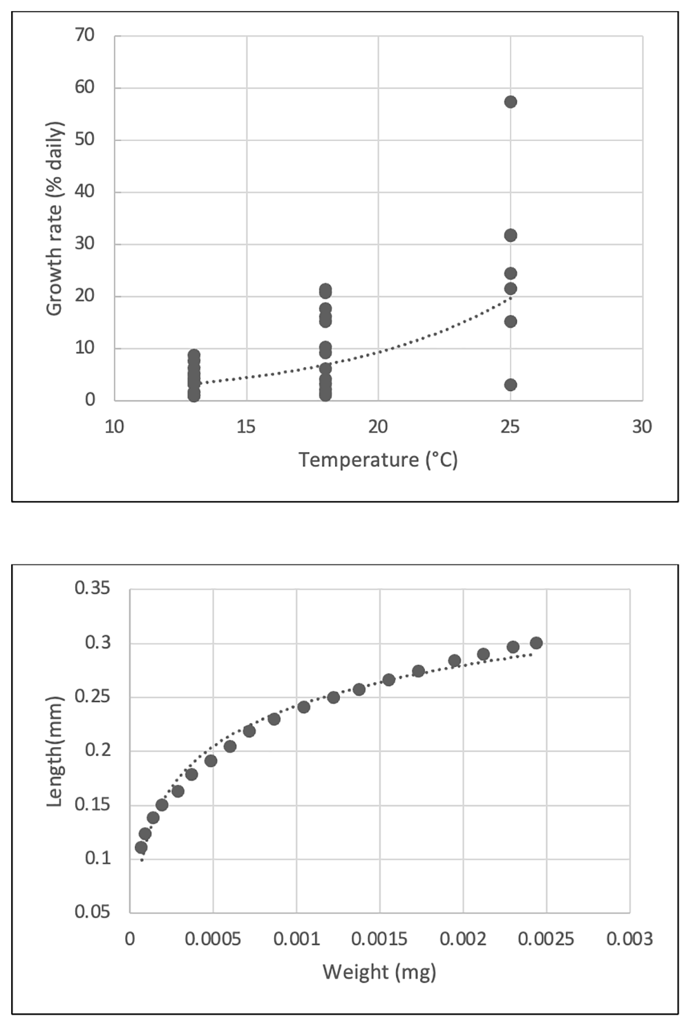
Figure 1. Growth rate and temperature (top) weight and length relationships (bottom) used for model parametrisation.
The forcing functions, i.e., current, salinity and water temperature, were downloaded from the CMEMS global ocean 1/12° physics analysis (x and y water velocities, sea water salinity; 6 hours, https://doi.org/10.48670/moi-00016) and from CMEMS Mediterranean sea physical analysis (temperature, ocean mixed layer thickness, hourly means, https://doi.org/10.25423/CMCC/MEDSEA_ANALYSIS_FORECAST_PHY_006_013_EAS4) for the year 2022 (1 April to 31 December) via Copernicus ‘my ocean viewer’, using map selection with coordinates spanning (lon: 12.00 to 14.00; lat: 44.00 to 46.00) and all vertical levels. Bathymetry with a 5 arc-second interval grid resolution was downloaded from GEBCO (gebco.net) and transformed the negative values to positives and to allow the recognition as an Opendrift bathymetry ‘reader’.
Simulations set-ups
O. edulis larvae were released from two areas, which were determined based on the following criteria: i) presence of shipwrecks (http://www.datiopen.it/it/opendata/Mappa_dei_relitti_in_Italia) and ii) presence of the species based on the map of presence/absence of the species available on EMODNET (https://emodnet.ec.europa.eu/geonetwork/srv/eng/catalog.search#/metadata/8e1a8ccc37da27c53c3d2db6bdd5a1efe39db8ea, most of the references for the Northern Adriatic refer to surveys conducted in the early 1990s).
The resulting areas were Wreck 1: 45° 17’ 24’’ N, 12° 59’ 24’’ E ; Wreck 2: 45° 16’ 48’’ N, 12° 34’ 48’’ E. The seeding was set to occur on a radius of 50 m around each wreck to allow for uncertainties in the exact position and seeding was set at 20 cm above seabed (assuming they would be on the wreck, and from observations of adults on raised substrates). Since Opendrift simulations can be set to last according to time (duration in time, number of calculation steps or final date), larvae were set to retire (reach settlement status) according the development time (the time needed to go from planktonic to settlement stage), which according to Rodriguez-Perez et al. (2021) and other previous research (Cole & Jones, 1939; Davis & Calabrese, 1969; Robert et al., 2017), is dependent upon temperature. In this case development time was used as ‘expiry date’ of the larvae, using it to set the simulation duration in time, and was calculated based on the median water column temperatures at the wreck site, assuming they would be representative of those that a larva would encounter. Simulations were done throughout the period April–December 2022, which was divided in fortnightly periods when simulations were set to end according to the different development times. Within each fortnightly period, 100 larvae were emitted daily at 18:00. Table 2 reports the median temperatures and development times (calculated using the equation in Table 1), for each larval seeding fortnight: these ranged from nearly one month in early spring to approximately one week in the warmest part of summer. Temperatures that were actually encountered by the larvae were quantified a posteriori based on actual trajectories.
Table 2. Median and standard deviation temperatures at the two seeding sites, development days required to reach settlement stage (month and days range considered).
Period
(fortnight) | April
1–14 | April
15–30 | May
1–14 | May
15–31 | June
1–14 | June
15–31 | July
1–14 | July
15–31 | Aug
1–14 | Aug
15–31 | Sept
1–14 | Sept
15–31 | Oct
1–14 | Oct
15–31 | Nov
1–14 | Nov
15–31 | Dec
1–14 |
|---|
Median
Temperature
(°C) | 10.9±0.5
10.9±0.5 | 11.9±0.5
11.9±0.4 | 14.1±1.6
13.7±1.6 | 16.3±2.4
15.8±2.4 | 21.3±2.8
20.7±2.7 | 22.9±2.8
22.6±2.7 | 25.3±2.6
25.1±2.6 | 25.7±2.3
25.4±2.3 | 26.3±1.9
26±1.9 | 25.8±1.4
25.7±1.4 | 25.3±1
25±0.9 | 23.7±1
23.6±0.9 | 21.6±0.7
21.5±0.5 | 21±0.7
21±0.4 | 20.5±0.9
20.4±0.6 | 17.7±0.9
17.7±0.8 | 14.7±1.1
15.2±1 |
Development
time (days) | 29.65 | 26.45 | 22.65 | 14.4 | 11.4 | 9.11 | 7.335 | 6.85 | 6.55 | 6.75 | 7 | 8.2 | 9.87 | 10.66 | 11.17 | 14.73 | 18.4 |
Statistical analysis
R (version 4.3) was used to open the .nc output files using ‘ncdf4’ (version 1.21) and create plots using ‘gtools’ (version 3.94). The code is available as Extended data (Bertolini, 2023b).
Results
Table 3 (Bertolini, 2023a) shows the actual temperatures encountered in the trajectories of the larvae and the depths of such trajectories.
Table 3. Temperatures (median ± standard deviation) and Depth (max; min)) of the larvae trajectories for the 100 larvae seeded in each fortnight at the two wrecks location (W1: Wreck 1; W2: Wreck 2).
Period
(fortnight) | Site | April
1–14 | April
15–30 | May
1–14 | May
15–31 | June
1–14 | June
15–31 | July
1–14 | July
15–31 | Aug
1–14 | Aug
15–31 | Sept
1–14 | Sept
15–31 | Oct
1–14 | Oct
15–31 | Nov
1–14 | Nov
15–31 | Dec
1–14 |
|---|
Temperature
(°C) | W1
W2 | 14.6±0.9
14.7±1.3 | 13.9±1.9
16.3±1.6 | 16.5±2.2
20.8±1.6 | 18±2.7
22.2±1.7 | 15.8±1.1
24.6±1.1 | 17.9±3.1
24.3±2.3 | 23.8±2.2
27±0.6 | 24.9±1.9
27.6±1 | 27.2±0.5
25.4±1.8 | 24.6±1.6
27.1±0.7 | 24.5±0.8
25.5±0.9 | 22.1±0.6
22.6±0.5 | 21.±0.2
21.1±0.6 | 21.4±1.1
21.7±1 | 18.2±0.7
17.9±1.6 | 15.8±0.7
14±0.7 | 13.3±1.7
13.3±1.9 |
| Depth (m); | W1
W2 | 31; 0.1
24,1;0.1 | 48.2;0.1
25.1;0.1 | 47.2,0.1
27.4;0.1 | 35;0.1
32;0.1 | 39.9;14
20;0.1 | 36;0.1
26.1;0.1 | 35;1.6
33.6;0.1 | 34.8;0.1
25;0.1 | 33.9;2
24;0.1 | 33;15.2
28.5;0.1 | 29;14.4
25;0.1 | 27.8;18
27;0.1 | 28,6;21
26;0.1 | 30.5;20
27;0.1 | 30.4;20
24.4;0.1 | 33;26
33;0.1 | 33;25
33;1 |
In terms of likely settlement areas, as evident from both wrecks, it is highly variable between the different seeding fortnights. Some differences can also be observed in terms of initial seeding locations: while seeding from Wreck 1 larvae go in every direction if the whole reproductive season is cumulated (Figure 2), when seeding from Wreck 2 they do not go to the NE to SE quadrant (Figure 3). This is also evident from the depths (Table 3), where larvae from Wreck 2 tend to occupy also shallower zones in all periods, whereas larvae from Wreck 1 in some fortnight only stays deeper (>10 meters). Generally, however, in both cases the larvae with a longer development time (cooler months, e.g., April and May, November and December) have the potential to settle further away.
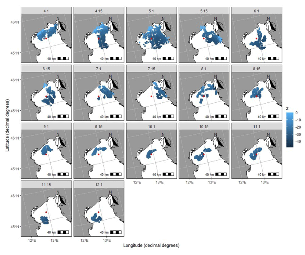
Figure 2. Results from the simulations from Wreck 1.
Each facet represents one fortnight (labels: month- day of simulation start). Dots represent potential settling locations and colours represent depth (z).
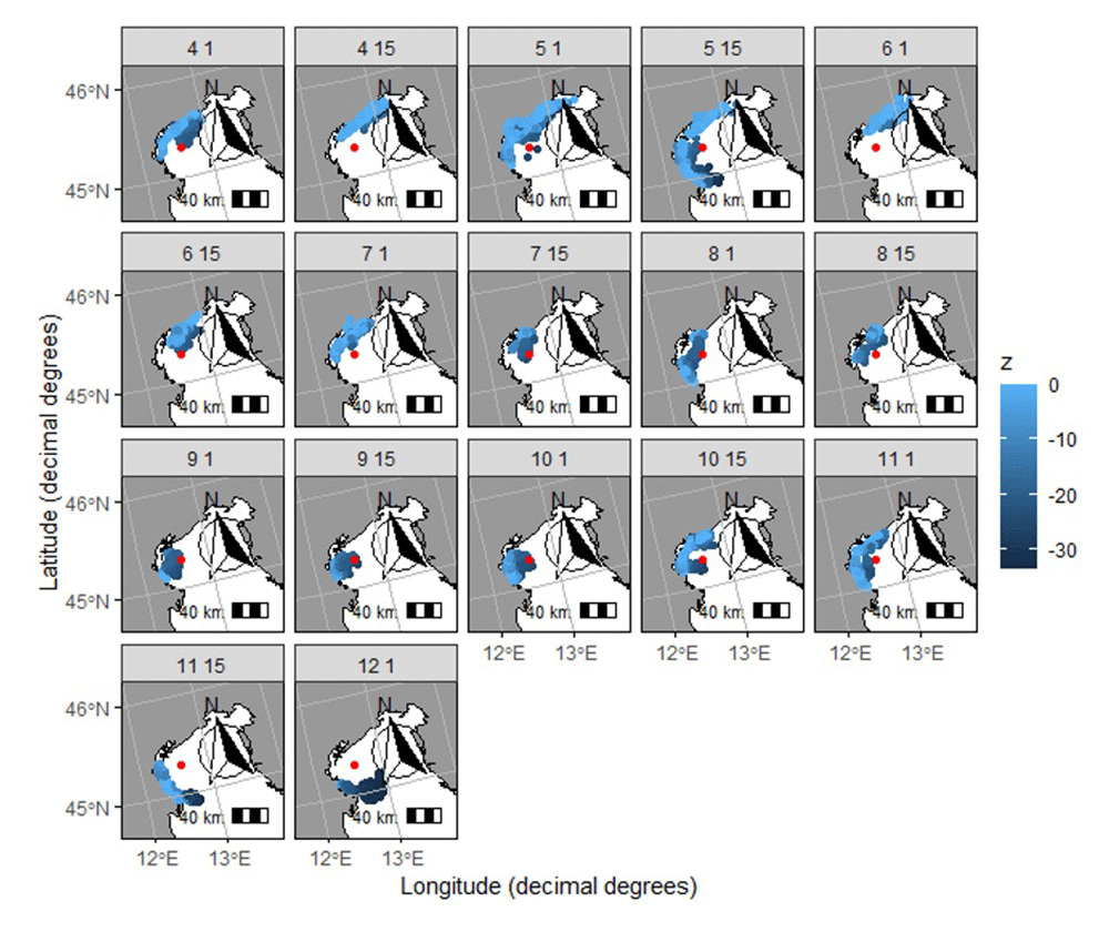
Figure 3. Results from the simulations from Wreck2.
Each facet represents one fortnight (labels: month- day of simulation start). Dots represent potential settling locations and colours represent depth (z).
Discussion
The results of this preliminary model-based study showed that the settling areas depend on the timing of the emission periods. The spatial distribution of the settling points matches the range of historical distribution from OBIS and observations of spat found in Caorle in summer of 2022 and shallow area of Pellestrina in the summer of 2023 (pers. Obs). Predictions of the settling areas of larvae sourced by Wreck 2 also suggest settlement inside the Venice lagoon, through the Chioggia inlet. Settlement of O. edulis was and is recorded on the inlets and the areas facing the inlets (Pellizzato, 1984 and Bertolini personal observation from summer 2022).
Shifts in spawning phenology may be a consequence of climate change (Dijkstra et al., 2011; Thomas & Bacher, 2018), which could, in turn, have consequences for the larvae dispersion. In this area, currents show a marked seasonal pattern, with NAd Gyre (anti-clockwise) being present in autumn (Artegiani et al., 1997). Therefore, the extension of the emission time window leads to a larger dispersion area, which, in turn, favours the genetic mix within the whole northern Adriatic.
The temperature dependence of swarming appears to be dependent by locations. Bromley et al. (2016) reports that the onset of spawning of Ostrea edulis occurs above > 15°C throughout its range with higher temperatures at the northern end of the range (Norway, Denmark) and lower temperatures (around 12°C), in some part of the Atlantic in the NE of Spain and in the Adriatic. Therefore, even if in our study at the beginning of April median temperatures at the wreck sites in the northern Adriatic were around 11°C it may still be possible that swarming occurred. In this study median temperatures were used for the seeding area and temperatures were not specific to each trajectory, with development time being fixed for each fortnight, which is a limitation of using a pre-existing module. Differences between the temperature used to estimate development time were up to 4°C lower compared to the actual temperatures of the trajectory in spring, equivalent to nearly 10 days of difference. In the period July-October the temperatures were more closely matching, however larvae released at Wreck 1 ended up in deeper water, which in the summer months were colder than median water temperatures expected at the original location. Consideration of depths and potential for temperature stratification at the area studied should therefore be added when determining the temperature to be used in calculation of development time, as this could be over- or under-estimated. An alternative would be to create another function in Opendrift that would allow stopping the simulation based on final size attained rather than by time, to allow more fine scale estimates based on single trajectories.
It should be pointed that what is modelled in this study is only the potential dispersal area. The longer the larval phase, the higher the mortality rate due to predation, while growth may also be affected by the actual availability of food resources: to this regard, the latitudinal West-East trophic gradient could decrease the probability the larvae released close to the Italian coast could settle on the other side of the Adriatic. Last but not least, the availability of suitable substrate (e.g., presence of hard substrate, conspecific cues, predator cues, biofilm (Kamermans et al., 2018; Potet et al., 2021; Smyth et al., 2020)), can also affect the outcome of the transition from the larval to the sessile stage of the life cycle.
In combination with this modelling approach scaled up to population, an integrated approach that includes sampling for larvae in the water column, checking settlement on substrates at different times, performing genetic analysis (e.g., paternal reconstruction (Monteiro et al., 2022)) and conducting broad scale surveys of remnant populations in the Adriatic, would be beneficial to better be able to preserve and restore the species–allowing to add suitable substrata in the right places and right time promoting the natural recovery (Kerckhof et al., 2018). While more experimental validation would be necessary, this setup using an open data and an open access existing modelling framework to predict larval settlement is promising and could enable upscaling and application for restoration and conservation purposes in other areas.
Ethics and consent
Ethical approval and consent were not required.