Having formally solved the problem for arbitrary boundary conditions in the preceding section, we now implement the boundary conditions for the configurations shown in Figures 1.3a–1.3d.
As already pointed out in the Introduction, the solutions for the configurations of Figures 1.3a–1.3b, that we are about to derive, with the boundary conditions corresponding to contact lines, describe unphysical displacement fields, diverging at the contact interfaces. We show that this can be cured by deriving a solution involving extended contact regions, using the Hertz contact deformations formalism. We show that even though the displacements differ between these approaches, the stresses near the center of the waveguide are in reasonable agreement.
4.1 Line contacts
4.1.1 Resting on a contact line. We start with the analysis of the simplest physical model, given by a cylindrical waveguide lying on an infinite plane, contacting (as a first approximation) only on a line. This is reminiscent of the famous Flamant solution with circular cross-section (see in particular [14, Problem 3 of Chapter 12]).
The boundary conditions are given by
where is the pressure with which the contact line is resisting the weight of the waveguide and 𝔭 the ambient pressure, taken to be constant. To put this into physical terms, we apply neither tangential nor radial forces, except for the contact line with the “contact wire”.
This model is particularly convenient, since the δ-distribution has a Fourier series expansion as
We find for the coefficients in the Michell solution
with
as follows from the condition Equation (3.13).
This last constraint implements the physicality of the calculations, since in the absence of other forces there can only be an equilibrium configuration if the integrated body force of the waveguide
matches the reactive force exerted by the plane, given by
The sum in (2.27) converges for coefficients (4.4)–(4.7), yielding
and further for the stresses
with
A representative plot of the stresses can be seen in Figure 4.1.
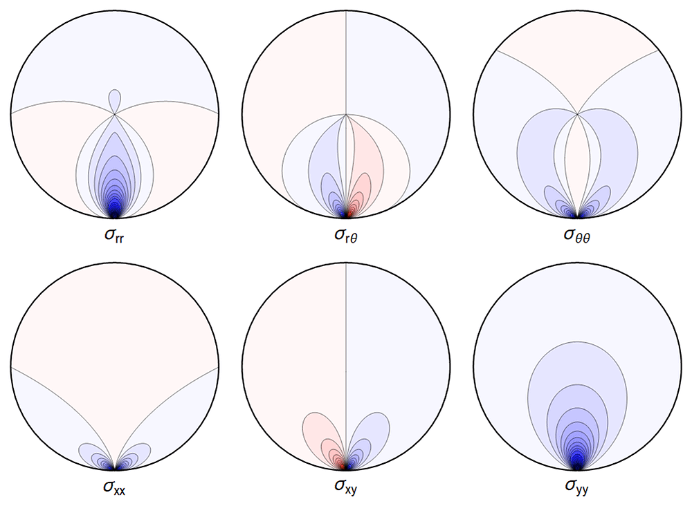
Figure 4.1. Typical plot of internal stresses for the case of a waveguide resting on an infinitely thin line, with unrealistic parameters arbitrarily chosen for illustration purposes listed in Table 4.1.
Table 4.1. Set of parameters chosen in our visualizations.
For conciseness, we express lengths in multiples of a, and pressure in multiples of the shear modulus μ, leading to dimensionless quantities for the remaining parameters used in numerical calculations.
| ρg | ν | 𝔭, κ, α | | = |
|---|
| 0.01 | 0.17 | 0 | 1 | 0.3 |
Here, and in all similar figures, shades of blue indicate compressive (negative) stresses, shades of red indicate positive ones, with darker colors encoding larger stresses.
Equation (2.28)–Equation (2.30) do not make sense, as the sum in Ξ does not converge. But one can find explicit expressions for ur and uθ by integration; the resulting formulae are lengthy and not very enlightening, therefore we did not include them here. Not unexpectedly, and similar to the Flamant solution [9, Chapter 8.4.7] , the singularity in the function A at r = a and cos θ = 1 leads to an infinite displacement there. Hence the boundary condition u(r = a, θ = 0) = 0 cannot be imposed. However, the displacements obtained by direct integration are finite away from the contact point, in particular near the center of the waveguide (cf. [16]). One can also truncate the series (2.28)–(2.29) which leads to finite solutions, illustrated in Figure 4.2.
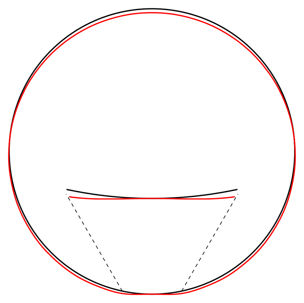
Figure 4.2. Illustrative deformation for the case of a waveguide resting on an infinitely thin line, after truncating the sums in (2.28)–(2.30) to n = 20, drawn in red.
The undeformed reference is drawn in black. Here and in similar figures below, the inset shows a magnified section around the contact point.
4.1.2 Squeezed between two lines. In a waveguide wound on a spool, consecutive layers of the waveguide press onto each other. The simplest model for this is a cylinder squeezed between two contact lines, with a pressure pushing from the top, as in Figure 1.3b. See also [9, Example 8–10] and [14, Problem 1 of Chapter 12], where a similar problem is modelled by superposition of three particular stress fields, including two Flamant solutions together with a uniform radial tension loading. The boundary conditions are given by
The calculation is completely analogous to the above, with the boundary condition enforcing
with the force-balancing condition Equation (3.13) now reading
Again, the physical interpretation is that now the force from above necessitates a reactive force from below larger than in (4.8) to achieve equilibrium.
Denoting by the right-hand sides of (4.12)–(4.14), the stress components read
with . Again, visualizing the result gives a clear picture. See Figure 4.3.
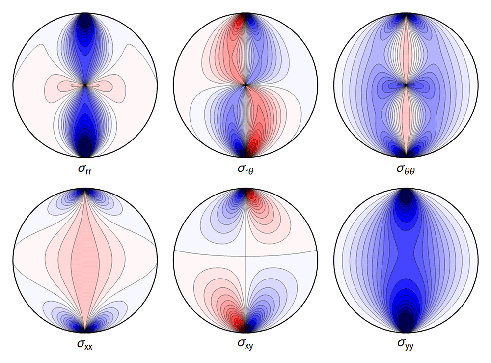
Figure 4.3. Typical plot of internal stresses for the case of a waveguide squeezed between two lines; same parameters and color coding as in Figure 4.1.
As before, the deformation diverges at the “contact wires”. A truncated sum is shown in Figure 4.4.
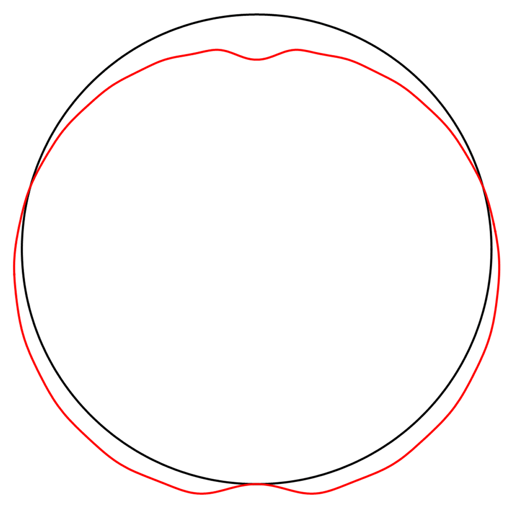
Figure 4.4. Illustrative deformation for the case of a waveguide squeezed between two lines, after truncating the sums in (2.28)–(2.30) to n = 20, drawn in red.
The undeformed reference is drawn in black.
4.2 Hertz contact deformations
In view of the above divergences, a better model for the contact between the waveguide and its support, or between neighbouring strands of the waveguide, is needed. A possible solution for this in linear elasticity is given by the Hertz contact deformation [17], with a modern derivation given by [10, Chapter 9].
To implement this we consider two cylinders contacting lengthwise. The contact region, which was previously described as a line, becomes a strip. On each cross-section, the contact point of the previous analysis becomes an interval (cf. [10, Problem 2 of Chapter 9]). The total force 𝔽 per unit length pushing two bodies into each other is now distributed over a region {x : −s ≤ x ≤ s}, where
with {ν, E, R} the material properties and radius of curvature of the body in question and {ν′, E′, R′} for the body in contact. In this model the pressure distribution over the contact region, which we denote by Py, equals
This can be restated in the form of boundary conditions
where
For the case of an infinite cylinder resting on a rigid plane, we simply take R′, E′ → ∞ and ν′ → 0.
Finding the cosine expansion of (4.28) is not obvious. Instead, we will approximate the Hertz profile with a step-function as in Figure 4.5, with straightforward cosine expansion, allowing us to find explicit expressions for the Airy functions and stresses in the settings discussed below. The half-width of the step function can be determined, based on the Hertz solution, to
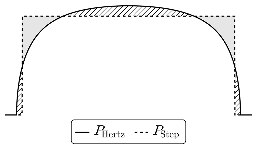
Figure 4.5. Comparison of the pressure distribution in the contact region for the exact Hertz solution (4.28) and an approximation using constant pressure in the contact region.
The shaded and dashed regions cause overshoot and undershoot in the displacement figures below.
via (4.25) and (4.29), ensuring a physically motivated boundary pressure distribution in response to external forces.
For the purpose of the GRAVITES experiment the key role is played by a) the change of length of the waveguide and b) the deformations near the center of the waveguide, where the core of the waveguide is located and where the photons propagate, with the energy of the waves decaying exponentially fast in the cladding. In Figure 4.10 and Figure 4.11 below we show a typical plot of differences between the point-contact solution and our variation of the Hertz-type solution. The figures make it clear that the differences are subdominant in the region of interest. In Figure 4.12 we further show that the difference between the Hertz-type solution and the step-function model is negligible for all our purposes. Our calculations show that both the point-contact approximation and the step-function approximation provide a good approximation for weak forces and away from the contact region, with a numerical comparison provided in Section 4.2.3.
4.2.1 Resting on a rigid plane. We apply the above to a waveguide resting on a plane, as in Figure 1.3a. Approximating the Hertz contact solution of Section 4.2 by a step-function of constant pressure for a single contact region from below leads to the boundary conditions
with Θ ≔ ΘHertz as defined in Equation (4.31), where for any set Ω we set
By assumption our boundary conditions for σrr are mirror-symmetric with respect to the vertical axis and 2π-periodic. We can write a general formula for the Fourier cosine expansion of their symmetrized sum. For ψ, Θ ∈ [0, π] we have,
When ψ = 0 we obtain the following coefficients in (2.27):
With condition Equation (3.13) reading
The summed expression for the Airy function is
where the subscript “single” refers to a single contact region, with
All the sums converge, leading to an admissible displacement field. The stresses and the displacements are shown in Figure 4.6 and Figure 4.7.
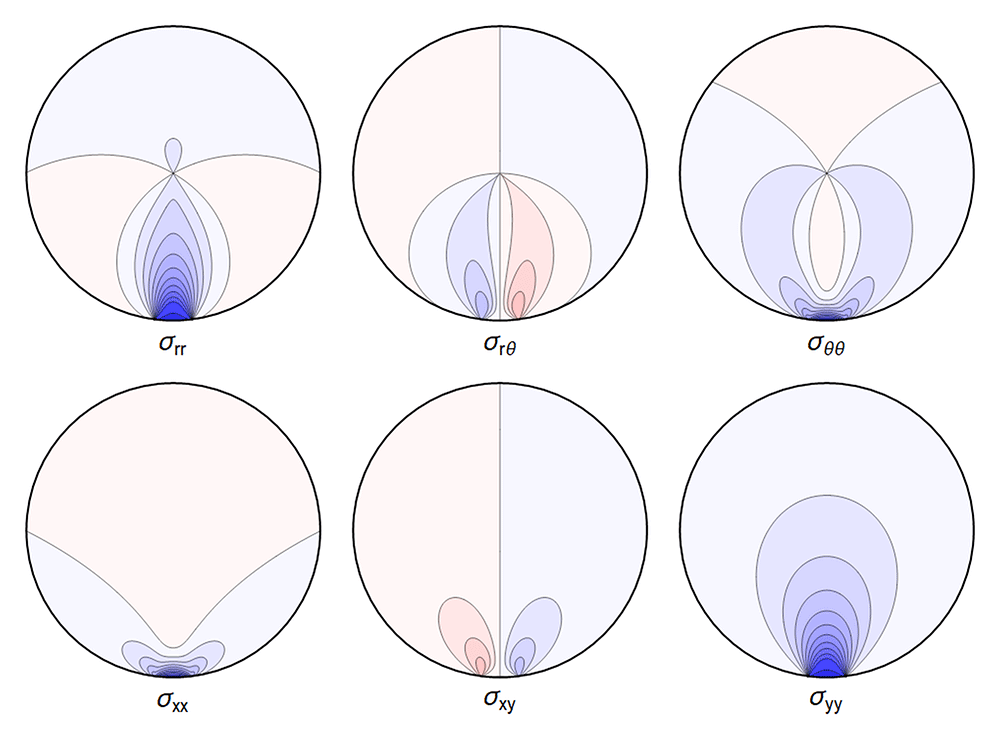
Figure 4.6. Typical internal stresses for a waveguide resting on an extended contact zone.
Here, and in the following figures, we use the same parameters and the same color coding as in Figure 4.1.
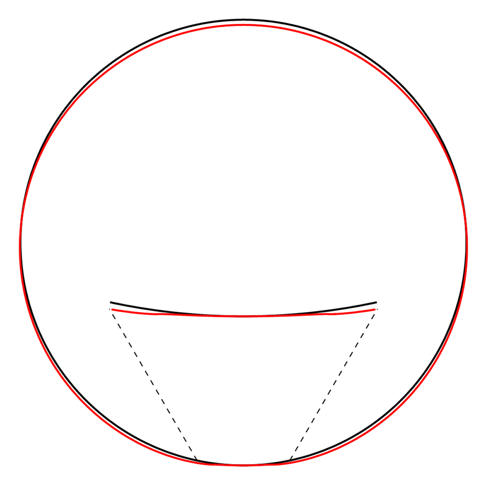
Figure 4.7. Deformation for the case of a waveguide resting on a rigid plane, drawn in red.
The undeformed reference is drawn in black. Here, and in similar figures that follow, the (barely visible) indentation is an artefact of the approximation illustrated in Figure 4.5.
4.2.2 Squeezed between two rigid planes. The next simplest description of a spooled waveguide is one with extended contact regions both above and below. We model this by squeezing the fiber between two rigid planes in the spirit of Section 4.2.1, i.e. boundary conditions
with Θ now an angle which approximates half of the contact region from below and the same from above.
The Fourier coefficients for the Airy function are found to be
with condition Equation (3.13) giving
The re-summed expression for the Airy function is
where
All the sums converge, leading to a finite displacement field. The stresses and the displacements can be seen in Figure 4.8 and Figure 4.9 respectively. Here, and in the plots that follow, the parameters are related to those of the two contact-lines case via the correspondence
which guarantees an identical integrated reaction force from the support.
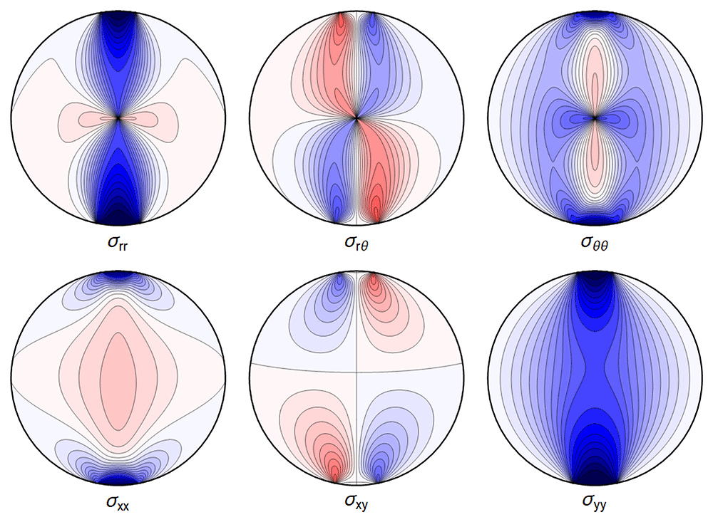
Figure 4.8. Internal stresses for the case of a waveguide squeezed between two rigid planes with extended contact region.
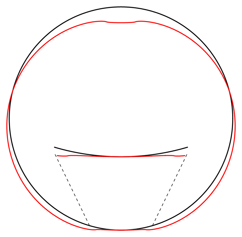
Figure 4.9. Deformation for the case of a waveguide squeezed between rigid planes of finite width, drawn in red.
The undeformed reference is drawn in black.
4.2.3 Comparing models. It is of interest to compare the different contact models we employed above, in particular validating the assertion that the step-function is a good approximation for the Hertz contact pressure Equation (4.27)–Equation (4.28), at least far from the contact region. In Figure 4.10 and Figure 4.11 we show the differences between the line contact models as discussed in Section 4.1 and the step-function approximation employed in Section 4.2 going forward, for the set of parameters given in Table 4.1. In Figure 4.12 we show the difference between stresses resulting from the Hertz contact model, calculated numerically, and our explicit solution using the step-function approximation.
We can quantify the differences away from the contact points by comparing the maximal values over the regions
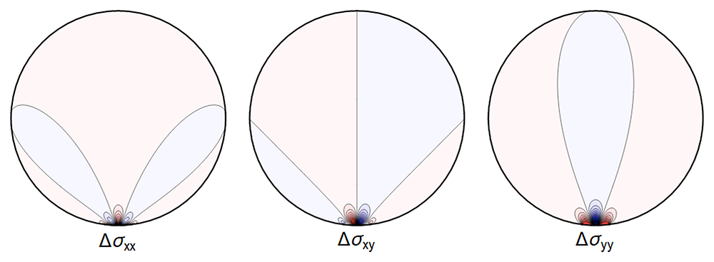
Figure 4.10. The difference ∆σ between the line contact Figure 4.1 and extended contact region Figure 4.6.
Here and in all figures comparing two sets of stresses, shades of blue indicate negative differences, shades of red indicate positive ones, with darker colors encoding larger differences.
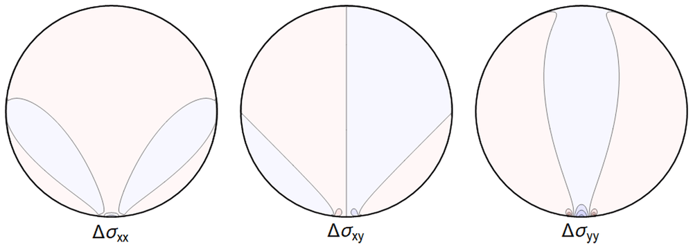
Figure 4.12. Difference ∆σ between the extended contact of Figure 4.6 and the stresses given by the full Hertz contact solution.
(Same color coding as in Figure 4.10 and Figure 4.11).
and
and setting
The results, for the parameters of Table 4.1 (used in all our figures), are shown in Table 4.2–Table 4.4.
Table 4.2. Relative differences, as defined in Equation (4.55), between the point-contact model and our approximation of the Hertz-contact model for the model of Figure 1.3a.
| σrr | σrθ | σθθ | σxx | σxy | σyy |
|---|
| ∆U1/2 | 2.9% | 4.4% | 5.5% | 11.7% | 6.5% | 2.9% |
| ∆U1/10 | 0.6% | 1.1% | 0.9% | 2.5% | 2.3% | 0.6% |
In the case of the line-contact model, a reasonable approximation is obtained in the central region for the values of parameters considered, if a 11% error is less than the measurement errors at hand. Comparing to the Hertz contact solutions, our step-function model gives errors of ~1% close to the center. Note in addition, that the chosen parameters for visualization correspond to much larger deformations than are expected to be relevant in physical applications, leading to more significant deviations.
Table 4.3. Relative differences, as defined in Equation (4.55), between the point-contact model and our approximation of the Hertz-contact model for the model of Figure 1.3b.
| σrr | σrθ | σθθ | σxx | σxy | σyy |
|---|
| ∆U1/2 | 2.4% | 9.9% | 7.7% | 11.0% | 17.2% | 3.9% |
| ∆U1/10 | 1.4% | 2.0% | 1.7% | 5.1% | 10.4% | 1.5% |
Table 4.4. Relative differences, as defined in Equation (4.55), between the Hertz-contact model and our step-function approximation thereof.
| σrr | σrθ | σθθ | σxx | σxy | σyy |
|---|
| ∆U1/2 | 0.7% | 1.1% | 1.4% | 3.0% | 1.6% | 0.7% |
| ∆U1/10 | 0.2% | 0.3% | 0.2% | 0.6% | 0.6% | 0.2% |
Of particular interest in this work is the effect on the length change given by Equation (3.17). The stress contributes to this change through the integral of its trace tr σ over the cross section of the body. In order to compare our models we evaluate the relative difference of the integrals over the cross-section of the trace of the stress tensor calculated in different models:
For the parameters listed in Table 4.1 this yields
We conclude that replacing the Hertz-contact model by a step function gives an excellent approximation, and that our simplest model, namely a contact along a line, can also be used to obtain fairly accurate numbers, for the change of length and for the deformations near the core of the waveguide, in spite of the divergence of the displacement field u at the contact line, depending upon the resolution needed.
We emphasize that this is a comparison of different contact models for a waveguide at a given height, and should not be confused with formulae such as Equation (5.2) below, where two configurations at different heights are compared using the same model.
4.2.4 Four contact regions. The calculations so far only take into account the neighbouring part of the waveguide pressing from above, ignoring the interaction between remaining neighbouring parts of the waveguide. The simplest model for this is presented in Figure 1.3c, with four contact regions for the waveguide, which we address now.
Using step-function boundary-stresses for the contact region gives
with Θ now an angle which approximates half of the contact region from below and the same from above and from the sides.
The resulting Fourier coefficients in the Airy function are
with
as by Equation (3.13). Note in particular the absence of a term proportional to as evident by comparing to the n = 1-term in Equation (4.35). This can be physically interpreted as the sideways pressures not contributing to the force balance in the vertical direction.
All the sums converge, leading to an admissible displacement field. The stresses and the displacement can again be illustrated graphically – see Figure 4.13 and Figure 4.14.
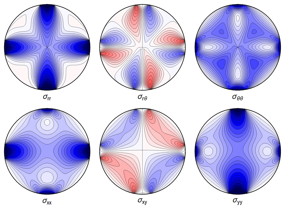
Figure 4.13. Internal stresses for the case of a waveguide squeezed between four rigid planes from below, above and the sides as depicted in Figure 1.3c, with extended contact region.
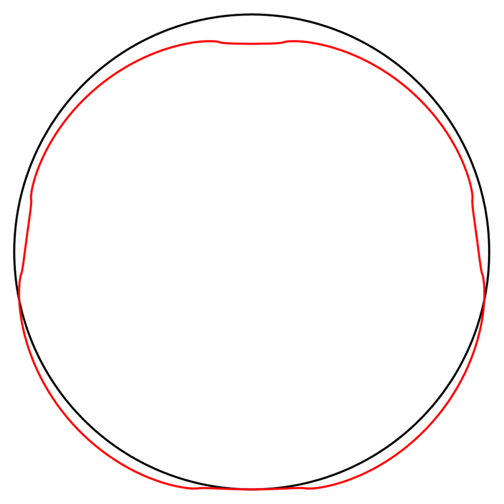
Figure 4.14. Deformation for the case of a waveguide squeezed between rigid planes of finite width as in Figure 1.3c, drawn in red.
The undeformed reference is drawn in black.
4.2.5 Squeezed between six rigid planes. Our final model for spooled waveguides is given by Figure 1.3d, which we model by imposing the boundary conditions
with Θ now an angle which approximates half of the contact region from below, and the same from above, and and from the sides.
The associated Fourier cosine series for the Airy functions has coefficients
with the force-balance condition Equation (3.13) leading to
equivalently
All the sums converge, leading to a finite displacement field. The stresses and the displacement are seen in Figure 4.15 and Figure 4.16.
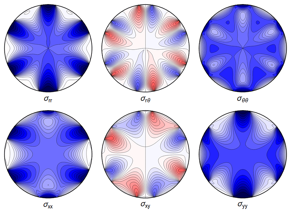
Figure 4.15. Internal stresses for the case of a waveguide squeezed between six rigid planes with extended contact regions, as in Figure 1.3d.
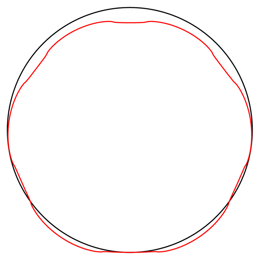
Figure 4.16. Deformation for the case of a waveguide squeezed between rigid planes of finite width as in Figure 1.3d, drawn in red.
The undeformed reference is drawn in black.










