1 Introduction
In recent years, new efforts to explore and study the Moon have been ramping up, exemplified by ongoing missions from several space agencies, like the Artemis program developed by NASA and ESA1. Although human missions are considered at later stages of these programs, using rovers to scout the surface remains the preferred method of exploration. Artificial intelligence (AI) is also expected to play a major role in these missions, as it can improve decision-making and traverse computations for a robotic mission on site2.
Within this framework, The EXPLORE Machine Learning Lunar Data Challenge was developed by the team of the EXPLORE consortium during the last quarter of 2022. The challenge required its participants to generate robotic traverses across a hypothetical lunar landing site, using AI and other computational techniques to survey the landscape and identify potential hazards. Here, we will briefly discuss the technical aspects of the challenge, to later describe and discuss the methodologies and results of the winning team. This work was developed as part of the EXPLORE project, whose main goal is to develop platforms that promote exploring space science data using AI and visual analytic tools.
1.1 Lunar exploration
Robotic instruments have been a cornerstone of lunar exploration since the initial stages of space flight. The first instrument that achieved a soft landing on the Moon was Surveyor 1 in 19673. This was simply a landing test, but even then, the instrument had a set of instruments that fed a central computer to control the landing, showing the importance of feedback and machine decision-making processes. During the era of the Apollo missions, the main focus was human exploration, and the vehicles were designed to be used by astronauts and not for autonomous control4. Nevertheless, during this period, in 1970, the Soviet Union developed the Lunokhod 1, the first moving instrument on the surface of the Moon5. The following years saw a rapid stagnation of lunar exploration, and when interest and activities were renewed at the end of the last century, the means of exploration shifted heavily from landers to orbiters. Several missions have been placed around the Moon in the last two decades, such as the Lunar Reconnaissance Orbiter (LRO)6, with the main advantages of having bigger coverage and time spans than rovers, greatly enhancing our knowledge of the lunar surface and subsurface.
In the last few years, interest in rovers has revived. The renewed intentions of taking humans to the Moon will be preceded by numerous rovers scouting the surface. A recent example is the rover Yutu-2, part of the Chang’e 4 Chinese mission7. This rover is the first to explore the far side of the Moon and is part of a more ambitious exploration program8. Upcoming vehicles are also being prepared, like the VIPER mission to the lunar south pole9. Finally, the private sector is starting to play an increasing role in exploration with missions such as ispace’s Hakuto-R Mission 1 carrying a rover from the Emirates Lunar Mission10. Overall, developing new ideas and technologies will be extremely important for the future of space exploration.
1.2 Machine Learning based planetary mapping
The application of Artificial Intelligence (AI), Machine Learning (ML), Deep Learning (DL), and Neural Networks (NN) in object detection extends significantly into areas of analysing satellite images, offering capabilities for monitoring and understanding planetary surfaces. By leveraging these technologies, it becomes possible to automatically identify surface features, both natural and man-made, from space with impressive accuracy and efficiency11–14. Deep Learning, in particular, has shown remarkable success in satellite imagery analysis due to its ability to handle the vast complexity and variability of data captured from orbit. Neural networks, especially Convolutional Neural Networks (CNNs)15–18, are adept at processing images often present at different spatial and spectral resolutions. These networks can distinguish subtle features across different terrains and conditions, making them highly effective for tasks ranging from mission planning to hazard detection and surface characterization. Integrating these technologies in satellite image analysis enables the automation of previously labour-intensive and time-consuming tasks, such as surface classification, change detection over time, and resource mapping. This capability is crucial for addressing global challenges in planetary sciences like crater counting19,20, boulder detection21,22, and more general surface segmentation23–25. By training neural networks on large datasets of labelled satellite images, these systems learn to detect objects and patterns of interest with high precision, opening up new avenues for research, policy-making, and commercial applications. The ability to process and analyse satellite imagery with AI and ML thus represents a significant leap forward in our capacity to observe and understand the planetary surfaces from a global perspective.
1.3 The lunar data challenge
Data challenges are useful to evaluate current and future space exploration problems as they seek to harness the scientific community to solve practical questions. For that reason, the EXPLORE Machine Learning Lunar Data Challenge was launched in 2022, in which the participants were challenged to use ML techniques to analyse the geological hazards of a potential lunar landing site and create a viable traverse for a robotic mission.
Since the challenge aimed to go beyond just processing data, three steps were established for the participants to follow in order to complete it successfully. The first step consisted of creating an object detection model for lunar landforms. In order to do this, the participant selected, created and trained a deep-learning model that could recognize the target landforms. For this challenge, we decided to focus on detecting craters and boulders since they would be the most immediate hazards for a rover. The second step was to apply the trained and verified model to the target location on the Moon, detecting the desired landforms. Finally, in the third stage, the participants integrated the prior results to generate a realistic traverse across some previously defined Regions of Interest (ROI).
To evaluate the results of the first steps, we reviewed the trained models, confusion matrices, and training scores. For the other two steps, we checked manually mapped landforms and traverses with the resulting labels, maps, and traverses developed by the participants.
The data challenge was open from September to December of 2022. In this work, we will showcase the methodology, results and discussion arising from the winning team of the challenge, as well as some considerations about the challenge itself.
2 Data selection and preparation
To accomplish the objectives of this ML data challenge, we decided to prepare two sets of data with different purposes. The first dataset is related to the data necessary to train the model in the first stage, with images collected from existing databases from scattered locations on the Moon. The second set of data corresponds to the zone selected to apply the model during the second and third steps of the model, the Archytas Dome in Mare Frigorifis (0.71◦ E, 55.71◦ N).
2.1 Selection of the region
As this lunar data challenge aimed to highlight these systems’ usefulness in exploring the Moon, it was essential to select a region that could be interesting to host a real robotic mission. Hence, the location should have a reasonable extension, good geological diversity, and scientifically interesting features. Furthermore, good data coverage and spatial resolution were needed to fully use the capacities of the ML techniques.
In the search for geological diversity, we decided to explore some landforms not usually studied in detail, such as intrusive igneous domes. They are the result of magma that cooled below the surface, eventually creating a noticeable landform due to its ascent through the crust or via faulting26. A list of intrusive domes was compiled by Lena et al.27, from which we selected the Archytas Dome as our study case since it fulfils the parameters described above.
The Archytas Dome is located south of Mare Frigoris in the vicinity of the rim of the Imbrium Basin (see Figure 1 for a simplified geological map of the zone). Similar to other intrusive domes on the Moon, it has a gentle slope of 0.25◦, a low altitude of 70 m, and a large diameter of 33 km27. The structure may be the result of the flexural deformation made by an ascendant intrusion, which stagnated as a laccolith near the surface28. The geologic diversity near the dome is high; close to the dome lies an elongated rille and a concentric crater, the latter being an uncommon type of crater with a poorly delineated inner rim and a flat floor. Wöhler and Lena28 suggest that this may be the result of an impact event during the emplacement phase of the laccolith. Furthermore, south of the dome, there is a sinuous rille that travels downhill from the Imbrium Basin rim, adding a more highlands-like set of rocks to the zone.
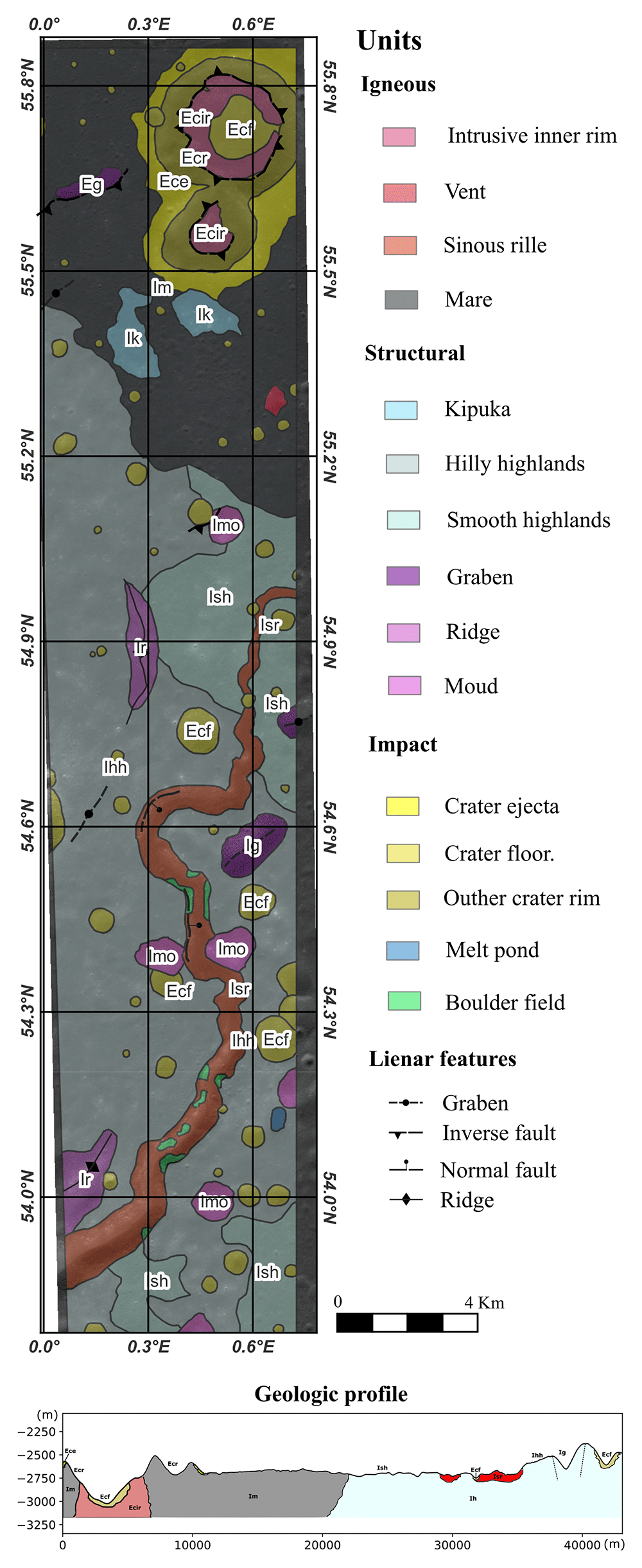
Figure 1. Geologic map of Archytas dome done in this work.
The selected location is 68 km large and 12 km wide, which is a reasonable coverage for a modern long-term robotic mission, e.g. Farley et al.29. All the geologic units mapped are dated as Imbrian (3.85 Gyr – 3.2 Gyr)30; hence, the region is heavily cratered and has experienced few resurfacing events. There is a clear accumulation of boulders near the rims of the larger craters and down-slope of the rille. The prior configuration provides plenty of boulder fields and craters to be recognised by the models to be trained by the participants.
2.2 Data preparation
A large amount of data is necessary to train ML models for image recognition31. This data should be representative of the target feature and its diversity, and the feature itself has to be labelled in every image. Craters and boulders are the most studied landforms on the Moon; therefore, a large amount of labelled data is already available (Figure 2 a, b).
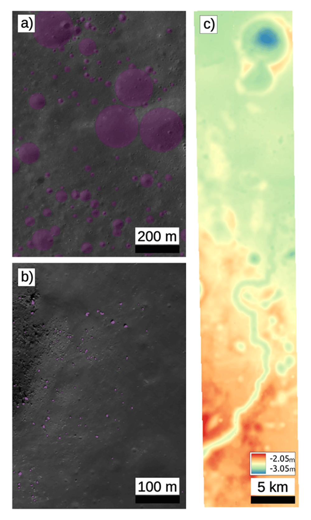
Figure 2.
a) Labels of crater from Fairweather et al.32; b) Labels of boulders from Watkins et al.21; c) Digital Elevation model of the Archytas Dome, elevation in meters.
The dataset of craters was collected from the work of Fairweather et al.32, who ran their model on images of the Narrow Angle Camera (NAC) onboard the Lunar Reconnaissance Orbiter (LROC)6, and detected craters with diameters between 20 and 500 m. As the Archytas dome is covered by a single NAC image, the scale of these labels suits our needs. We compiled 3257 labelled images with craters of different sizes and shapes, although all of them were simple craters. The dataset of boulders was collected from Watkins et al.21, which also detected these landforms in NAC images. The size of the boulders is naturally smaller than craters, ranging from 1 to 5 m. We compiled 9555 labelled images with boulders and boulders fields. Later, these datasets were randomly divided into test, valid, and training groups, containing 10 %, 20 %, and 70 % of the data, respectively. A list of the LROC images used for this purpose can be seen in Table 1.
Table 1. Images used to obtain the labels for the training of the model.
| Class | Label Type | Instrument | Image Name | Source |
|---|
| Crater | Bounding box
+ polygon | LROC NAC | M112963850lE,
M1288076949lE,
M1320016983lE,
M1325197569lE,
M1338833866lE,
M1361391010lE | Fairweather
et al. (2022) |
| Boulders | Bounding box
+ polygon | LROC NAC | M1108182629LE,
M1108182629RE,
M1259058367LE,
M150633128LE,
M150633128RE,
M152770233LE,
M152770233RE,
M165645700LE,
M165645700RE,
M165998991RE,
M181065865LE | Watkins,
Ryan (2019) |
For the data regarding the Archytas domes, we also used NAC images. The M1103544450LE and M1103544450RE takes were downloaded from the Lunar Orbital Data Explorer and processed up to map-projected images using the software ISIS33. Finally, a digital elevation model with a spatial resolution of 3 m was computed from the prior images using the Ames Stereo Pipeline (ASP)34 (Figure 2c).
2.3 Ground truth
To evaluate the fidelity of the ML model after its application to the Archytas Dome zone, it was necessary to compare it with a ground truth. As the existing databases do not cover the location, we created our own set of labels for craters and boulders. This step was made manually in QGIS; we created a squared grid to cover the area better and labelled features with sizes and shapes similar to those of the training sets of data. In total, we collected 586 craters and 746 boulders.
3 Methods
The solution proposed by the winning team to solve the three steps of the challenge was divided into three phases respectively: a network is trained to segment and predict boulders and craters on a general lunar surface, then the network is used to predict these obstacles on the Archytas Dome area of the Moon, lastly a traverse is calculated to reach certain ROIs while avoiding obstacles and inaccessible areas computed in the prior steps. The full process of the methodology is represented in Figure 3 and discussed in detail below.
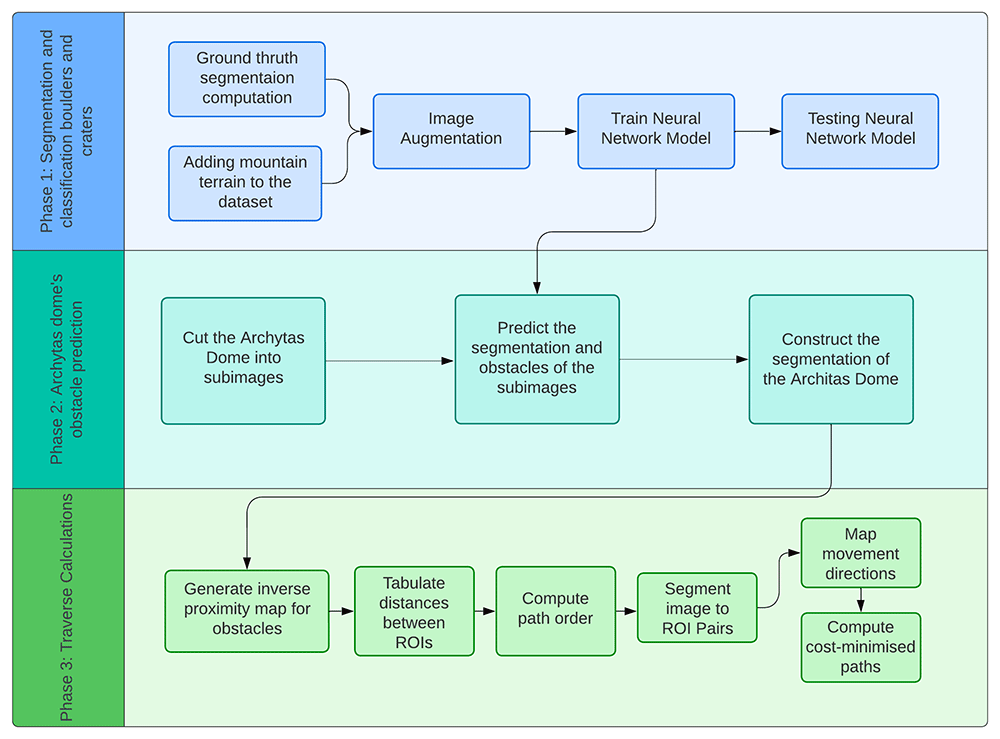
Figure 3. Flow diagram of each phase of the project; 1) segmentation and classification, 2) obstacle prediction, and 3) traverse calculations.
3,1 Segmentation and classification of boulders and craters
3.1.1 Data pre-processing. Neural networks aim to identify objects and their positions in an image, segmenting them into the desired distinctions. The ground truth of the segmentation is computed by unifying a few points of the object contours and then identifying the outside pixels as terrain and inside pixels as craters or boulders.
The images in the dataset constructed for the initial training contained boulders and craters of different sizes, which were resized to fifty-by-fifty pixels due to the neural network hardware requirements. The images are augmented with random translations and scales to reduce the number of boulders and craters of similar shape and size centred in the images. We applied additional shear values, random rotations, and vertical and lateral image flipping to increase the robustness of the network.
We supplemented the dataset with augmented images from Mt. Marilyn35–37 to improve the robustness of the model by adding topographic variations to the boulder and crater images.
3.1.2 Neural Network Architecture. The main task of the challenge is to classify boulders and craters on the lunar surface. Two different models, a Convolutional Neural Network (CNN) and a Vision Transformer (ViT), have been proposed and compared. A CNN learns the importance of the different elements of an image by assigning them weights and biases38. A ViT uses images divided into patches and considers the order in which these are given39. For an image representing a boulder or a crater, the network predicts its segmentation, whereby each image pixel is classified as either boulder, crater or terrain. The model uses an Adam optimiser and a cross-entropy loss, where the overall loss is minimised during training. The model training and testing, as well as the data handling, is executed by using Python, Pytorch and Jupyter Notebooks40.
3.2 Prediction of obstacles in the Archytas Dome
The second step of the challenge required the implementation of the trained model to the NAC image of the Archytas Dome zone. Due to limitations in the computational resources, especially the memory, we segmented the image of the Archytas Dome into smaller fifty-by-fifty pixel sub-images to pass through the network. The network classified each pixel as boulder, crater or terrain, and then the classified images were joined back together to the dimension of the original NAC image.
3.3 Traverse calculations
For the third step, the calculation of a lunar traverse, our solution aimed to develop an efficient methodology for generating paths that avoid obstacles and reach pre-selected regions of interest (ROI) by combining various algorithms within QGIS. A non-exhaustive list of existing path-generating methods and algorithms include: 1D Convolutional neural networks41, A*, D*, rapidly exploring random trees (RRT), potential fields42, Dubins’ paths, and Hamilton- Jacobi-Bellman methods43. Our simplified approach to this problem involved weighted ROI path selection and optimal traverse calculation requiring multiple image processing steps.
The QGIS44 raster terrain analysis was initially applied to the DEM NAC Archytas image to compute slopes above fifteen degrees. This image was then converted to a binary raster image and combined with the boulder and crater images to form an obstacle map. In our reduced complexity approach, the minimum path was found by creating a map of cumulative ROI distance costs and obstacle proximity distances to act as pseudo-topography for the r.drain algorithm (available in the QGIS GRASS package), generating vectorised least-cost paths.
Repeating the above steps for all ROI pairs is computationally expensive and, as such, the ROI path order is automatically pre-selected based on a cost-minimised route based on ROI distance and ROI importance (low, medium, high). This calculation is achieved by forming a list of Cartesian distances between all pairs of ROIs via the QGIS ‘Shortest line between features’ algorithm, adding ROI importance, and then applying our developed Dijkstra-based algorithm45 to compute the cost-minimised-path from the ‘Start’ to ‘End’ ROI.
The GDAL raster distance proximity algorithm is applied to pre-compute obstacle distances for the whole map with geo- referenced coordinates. The obstacles are clipped by subtracting the binary image, and the resulting image is inverted to give the highest weighting closest to the obstacles.
The map is segmented for each ROI pair, and cumulative costs and movements between the ROIs are found by the QGIS r.cost algorithm (Figure 4) before generating the paths via the QGIS r.drain algorithm, which are then combined to form a single traverse.
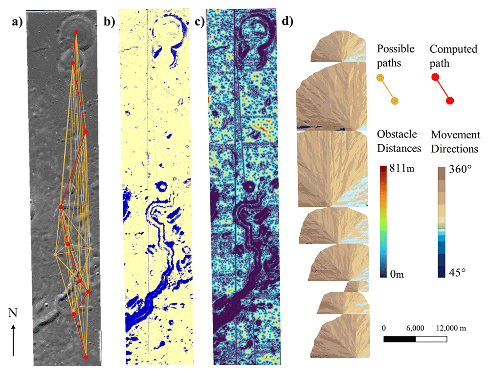
Figure 4. Steps to compute the optimal traverse.
a) Dijkstra weighted ROI path selection. b) Binary obstacle image (blue obstacles, yellow non-obstacles). c) Object proximity distances. d) Least cost movement directions.
4 Results
4.1 Boulders and craters segmentation and classification
We tested four models to predict boulders and craters across the Archytas Dome, and the results are summarised in Table 2. Via image augmentation (Subsection 3.1.1), the original dataset was doubled for the first three models and expanded eleven-fold for the fourth model. Figure 5 shows each model’s heatmap, while Figure 6 shows the second phase prediction of boulders and craters across the Archytas Dome. Vision Transformers (ViTs) and Convolutional Neural Networks (CNNs) both achieved image segmentation. From the results, we can see that a convolutional neural network works best with a segmentation problem, likely due to its general purpose backbone39. Adding learnable weights to the classes does not seem to increase the model’s overall score, but balances out the accuracy of the categories. Expanding the dataset improved the network’s robustness as the network could observe a larger variety of obstacles. This is particularly noticeable in the prediction of obstacles of Archytas Dome in the second phase (Figure 6).
Table 2. Model results summary of F1 scores.
Visual Transformer (ViT), Convolutional Neural Network (CNN), CNN with class weights, CNN with eleven times larger dataset.
| Model | F1 (%) |
|---|
| ViT | 62.31 |
| CNN | 71.44 |
| CNN with class weights | 70.69 |
| CNN with larger dataset | 75.46 |
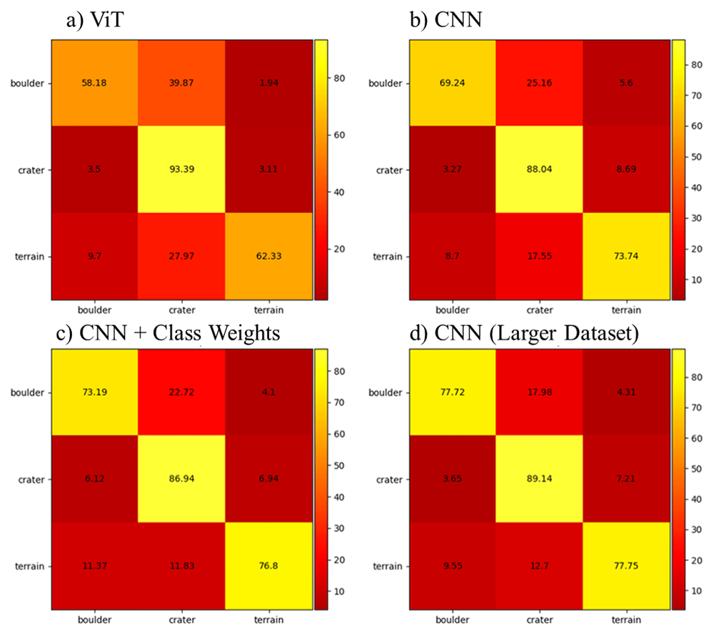
Figure 5. Model heatmaps.
a) Vision Transformer (ViT), b) Standard CNN, c) CNN with class weights, d) CNN with a larger dataset.
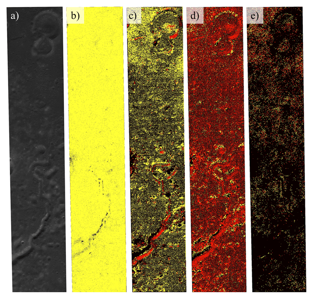
Figure 6. Results of the obstacle prediction phase for terrain (black), boulders (red), and craters (yellow).
a) Input NAC image, b) ViT, c) CNN, d) CNN with class weights and e) CNN with a larger dataset.
4.2 Traverse calculations
The applied methodology successfully computed a ~68.2 km long object avoidance traverse weighted between the start and end locations, reaching one low priority, four medium priority, and two high priority ROIs (Figure 7). The traverse could not be applied to the full set of initial ROIs due to two image artefacts in the DEM acting as slope barriers. The traverse does not cross any boundaries, and due to the stage two results, boulders and craters were not included in the final object avoidance image.
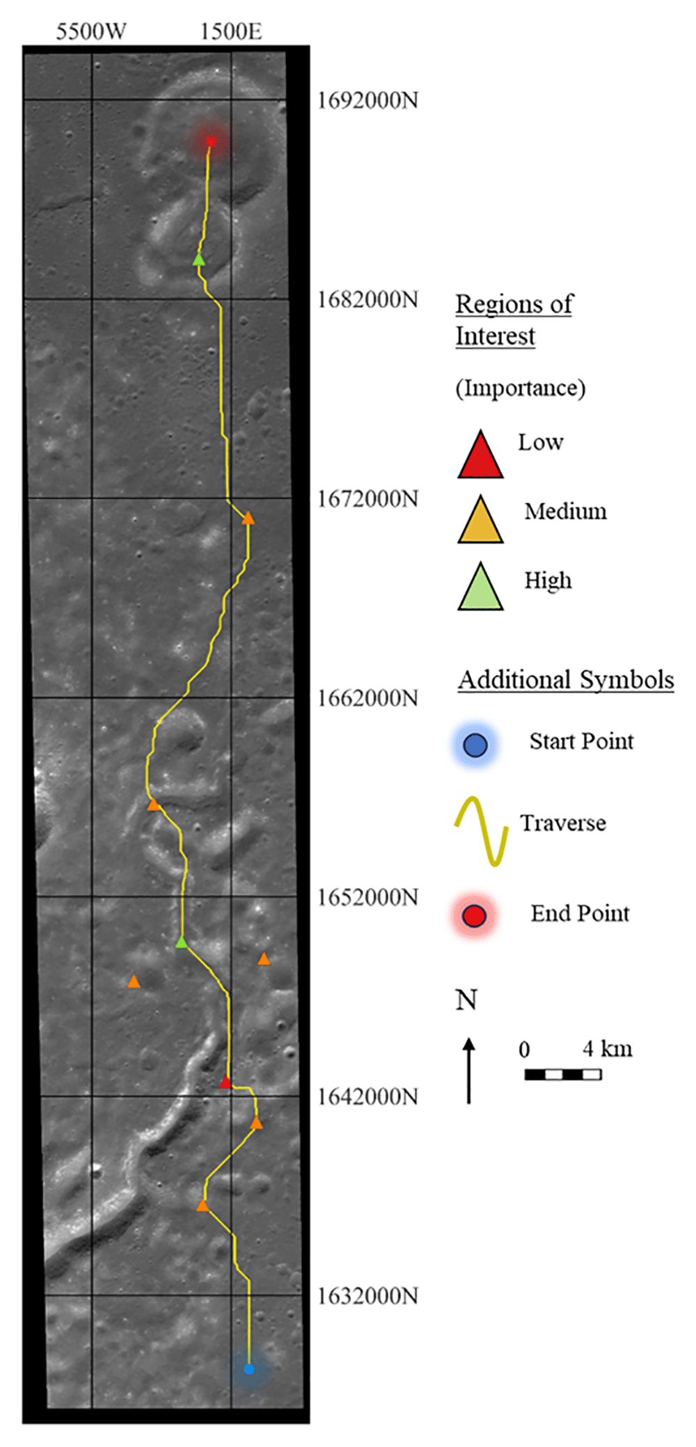
Figure 7. Automated minimised path length lunar traverse, avoiding slopes above fifteen degrees and contacting regions of interest around the Archytas Dome region.
5 Discussion
5.1 The model
The initial data has very similar features whereby the obstacles are centred in the image and have similar proportions with respect to the image size. This led us to augment the data with rotations, translations and scaling to acquire images of many types of boulders and craters. The visual transformer gives the least successful results due to its patching scheme. Meanwhile, a CNN learns how to give importance to the different areas of an image in no particular order with learnable weights and biases. Images of Mt. Marilyn have been added to the dataset to help the model distinguish obstacles on flat terrain from geologically mountainous terrain. Additionally, the model accuracies are also reduced due to the highly imbalanced dataset with more terrain than boulders and craters. The addition of weights balances the accuracy of the classes but not the overall F1 score. Enlarging part of the dataset images would greatly improve the F1 score in the first phase but the mountain chain south-west of the Archytas Dome would be fully identified as either a crater or a boulder. The addition of samples in the dataset improves the performance of the model due to the high number of possible craters and boulders. The Archytas Dome has been downsized and divided into smaller images due to its incompatibility with the square-shaped images of the first phase and its large size which does not follow the hardware constraints.
5.2 The traverse
The computed traverse methodology successfully computes weighted paths between ROIs automatically46. However, the cost-minimised path is based on maximum distances from objects (steep slopes), suggesting that there is scope to reduce the total path length with a traverse that comes closer to objects. The ROI order is pre-computed using a Dijkstra-based algorithm to reduce computational costs via a fully connected graph of distances between all ROIs. The complete path is not totally optimised as these distances assume straight-line paths, which do not account for the re-routing distances necessary for object avoidance. The cost-minimised traverse takes the ROI path as an input vector, where the path selection algorithm does not automatically allow paths to return to an ROI, preventing the automated addition of two medium-priority ROIs. The ROI weights are computed based on subtracting distances, which require arbitrary tuning, and are bounded by the minimum allowable distances of positive values, and do not give options to ensure a certain number of ROIs are reached. Our fully automated approach accomplished the traverse computations using simple QGIS functions and a bespoke Dijkstra-based algorithm; future directions should seek to overcome our method limitations and explore additional realistic constraints such as accounting for terrain roughness, minimising total slopes travelled, maintaining sunlight exposure, and including potential distance limitations for communication relays.
5.3 The challenge framework
Apart from the results of the winning team, we can draw some lessons from the organization and development of the data challenge itself. The number of participants was low; around six teams registered for the activity, of which two presented results, and only the winning team provided a meaningful approach to solving the challenge. Although the results of the winning team were consistent and demonstrated a good understanding of the challenge, the limited participation indicates missions overlooked during the challenge conception.
One explanation for the lack of participants was the low diffusion time of the challenge. After launch, we presented the challenge in several conferences, forums, and academic groups focused on machine learning, but earlier dissemination could have given potential participants more preparation time. Another obstacle to achieving larger project participation may be the high challenge complexity. We found that the majority of the participants needed help with integrating the different steps of the challenge. Building a rover traverse from real environmental conditions is complex and multidisciplinary; hence, the teams must be equally diverse. The successful team comprised a computer engineer and a geophysicist, each focusing on the machine ML and traverse computation, respectively. This three-step challenge configuration likely discouraged individual participants as it required knowledge of multiple disciplinary backgrounds. Defining more constrained activities or goals may be more beneficial for future data challenges.
A technical problem that arose was the training data quality. The mixed results obtained by the winning team in the Archytas Dome could be partially related to the training data provided by the EXPLORE team. The combination of labels for both craters and boulders is likely suboptimal due to the great difference in size between both landforms, ranging from craters with hundreds of meters in diameter to boulders that only occupied a couple of pixels on the image. Another factor may be the difference between the images used for the training dataset and the one of the Archytas region. Several factors may vary from one image to the next, from the illumination to the textural properties of the rocks. As observed in highly illuminated slopes, a big variance from one data set to another could cause poor model behaviour. A more consistent training dataset and using one type of landform would likely allow participants to achieve better results.
6 Conclusions
The EXPLORE Machine Learning Lunar Data Challenge was an interesting activity to test the use of ML techniques to solve real problems faced in lunar exploration. In the search for replicating a semi-real scenario of exploration, the complexity of the challenge escalated beyond a point where non-specialised users could not participate in the challenge effectively, resulting in a low participation by the public. Although a simpler challenge would have attracted more participants, it is worth noting that the winning team successfully understood and delivered solutions for the three proposed steps. Even if those results could be improved by a better training dataset or simpler tasks, their approach proves the usefulness of ML techniques in the future of planetary exploration.
The winning team constructed a neural network that can locate the position of boulders and craters, and successfully created an automated system to compute a cost-minimised path targeting weighted regions of interest that avoids obstacles such as slopes above fifteen degrees, boulders, and craters. This solution was based on connecting several QGIS functions and writing a bespoke Dijkstra-based script. The process relied on the cost-to-obstacle calculations and initial path selection from straight-line distances; the overall method was not fully optimised for minimising path lengths but may still be a useful tool for automatically generating traverse paths.
Ethics and consent
Ethical approval and consent were not required.